Hybrid Forecasting Techniques for Renewable Energy Integration in Electricity Markets Using Fractional and Fractal Approach

1  Introduction

The growing integration of renewable energy into electricity markets has introduced significant challenges and opportunities. With the increasing deployment of solar, wind, and other renewable sources, power systems are experiencing a transition from traditional centralized generation to more decentralized and variable power generation. Forecasting approaches have experienced multiple paradigm shifts in recent years. From the dominant position of classical statistics, machine learning (ML) has come into prominence over the last decades, with even more recent advances of deep learning (DL). Each shift in forecasting methodology was driven by a similar motivation, which is the necessity to model the increasing variability and nonlinearity in data [1,2]. Classical methods such as time series models (ARIMA, ETS) are more interpretable, easier to understand and implement, and may be sufficient for short-horizon tasks [3]. However, they usually rely on linear assumptions that can be restrictive for complex, non-stationary signals. ML models (decision trees, random forests, support vector machines (SVM), etc.) can account better for nonlinearities, and DL approaches. In a similar sense, the shift to renewables is essential to reduce carbon emissions and achieve sustainable energy goals, but also creates numerous challenges in terms of grid stability, demand-supply balancing, and electricity price volatility [4].

The efficiency of electricity markets in the future energy world, therefore, also primarily depends on the existence of accurate forecasting models. The forecasting models can forecast energy consumption, production, and market trends, thus enabling grid operators, energy traders, policymakers, and other stakeholders to make informed decisions [3,4]. In the meantime, the volatility and intermittency of renewable energy make this task more difficult and require advanced forecasting techniques beyond those traditionally used [5].

Traditional approaches use statistical techniques such as ARIMA and ETS, wherein the time series are modeled as functions of their lagged values. Though they are utilized today (when short-horizon prediction is necessary), such models basically circumvent the nonlinear character and other complex dependencies, as can be seen among the features of renewable energy generation [6]. For the purposes of evading the quirks of statistical modeling, scientists started to develop ML and DL methods for forecasting because of their inherent capability to fit complex relationships and to harvest rich information from huge data. Various approaches were used to accomplish this, and models such as ANN, SVM, and LSTM networks were reported to be of greater accuracy for predicting energy demand/generation [7]. Even these approaches, however, have drawbacks like high cost of computation, overfitting, and demand for a huge amount of training data.

Hybrid approaches are one of them that have become very popular over time. Hybrid models are simply a collection of a number of forecasting models, which work in conjunction with each other to leverage the strength of each and also enhance forecast accuracy and sensitivity to market patterns. One example is the coupling of statistical forecasting models and deep learning networks (CNNs, LSTMs) that can contribute to better linear and non-linear trend identification for more accurate and robust forecasts [8–12]. Other hybrid methods using ensemble-based techniques are ensemble learning, wavelet transforms, and optimization algorithms [13,14]. They typically work better than traditional methods but also have drawbacks in model interpretability, integration complexity, and computational efficiency.

In this study, we propose FFDEM (Fractional–Fractal Deep Ensemble Model), a hybrid approach that combines fractional long-memory (FARIMA), fractal roughness (MFDFA), and deep learning algorithms (CNN-LSTM/stacking). The dual injection of long-range dependence and multiscale roughness is what sets FFDEM apart from previous hybrids, and what causes the observed error reduction. In the design and development of FFDEM, fractional-order statistical models, fractal-based feature engineering, and deep learning architectures are all designed to work towards improving the forecast accuracy of renewable energy generation. Fractional autoregressive integrated moving average (FARIMA) and fractional exponential smoothing (FETS) models are investigated for the purpose of capturing long-memory dependence in energy time-series, and multifractal detrended fluctuation analysis (MFDFA) is employed for intermittency analysis of renewable energy generation. This paper will present and explore the viability and effectiveness of hybrid forecasting techniques for renewable energy integration in electricity markets. We also benchmark with transformer and decomposition-style long-horizon forecasters (e.g., Informer, Autoformer, FEDformer) as well as recent neural operators such as TimesNet. The key contributions of this research are as follows:

•   A hybrid framework melding ML/DL with fractional-order statistics and fractal-based feature engineering to enhance forecasting accuracy and efficiency.

•   A comprehensive comparative study of hybrid models using real market datasets.

•   An assessment of forecasting impacts on grid stability, energy trading, and risk management.

•   A critical review of current limitations and practical recommendations for future models.

•   Empirical validation of the proposed approach via case studies and quantitative analysis.

2  Related Work

Renewable and market forecasting have advanced rapidly in recent years. Comprehensive reviews catalog progress in photovoltaic (PV) forecasting and deep learning pipelines, emphasizing data quality, exogenous drivers, and evaluation protocols [2,9,15]. Concurrently, domain studies continue to motivate high-fidelity forecasting by linking prediction quality to market viability and planning in high-renewable settings [16]. Beyond point accuracy, recent works advocate reliability and robustness through probabilistic treatment and uncertainty quantification (e.g., Gaussian-process and tree-based methods adapted for calibrated predictive distributions) [7,17].

Modern neural approaches extend classical baselines by exploiting temporal hierarchies, exogenous weather, and transfer across locations or markets. Deep hybrids (e.g., CNN/LSTM stacks) and transfer-learning setups have improved short-term market and generation predictions by learning multiscale patterns while reusing representations across datasets [4,9,18]. Deterministic forecasting guided by multi-location meteorology demonstrates additional gains when spatial context is injected at training time [19]. In parallel, demand-side and load-focused studies report accuracy improvements from tailored deep models and careful data engineering, further underscoring the role of inductive bias and exogenous features [14,20]. At the operations interface, recent work links forecast design to market objectives and decision quality. Value-oriented forecasting integrates market structure into the learning target and loss design to improve downstream clearing outcomes.

Reinforcement learning has also been combined with time-series predictors to handle uncertainty and adapt bidding/dispatch actions in the presence of variable renewables [11]. These directions highlight the need for forecasting models that are not only accurate but also decision-aware and robust under distribution shift. Despite these advances, two gaps remain. First, long-memory and intermittency—core properties of renewable generation and price series—are often addressed implicitly via deep architectures rather than through explicit statistical descriptors. Second, hybrid systems rarely fuse such descriptors with learned representations under a leakage-safe ensemble. The framework in this paper targets these gaps by integrating fractional-order statistics and multifractal descriptors with neural sequence models in a unified, interpretable ensemble, complementing the trends above while remaining compatible with probabilistic and decision-aware extensions [13,21].

The proposed FFDEM which fuses fractional long-memory (FARIMA), fractal roughness (MFDFA), and deep learners (CNN–LSTM/stacking). This dual injection of long-range dependence and multi-scale roughness is unique to FFDEM among prior hybrids and underlies the achieved error reductions. Recent transformer and decomposition-style forecasters (Informer, Autoformer, FEDformer) and neural operators such as TimesNet set strong baselines for long-horizon series; we benchmark these models under matched settings. Table 1 summarizes representative techniques, highlighting strengths and limitations.

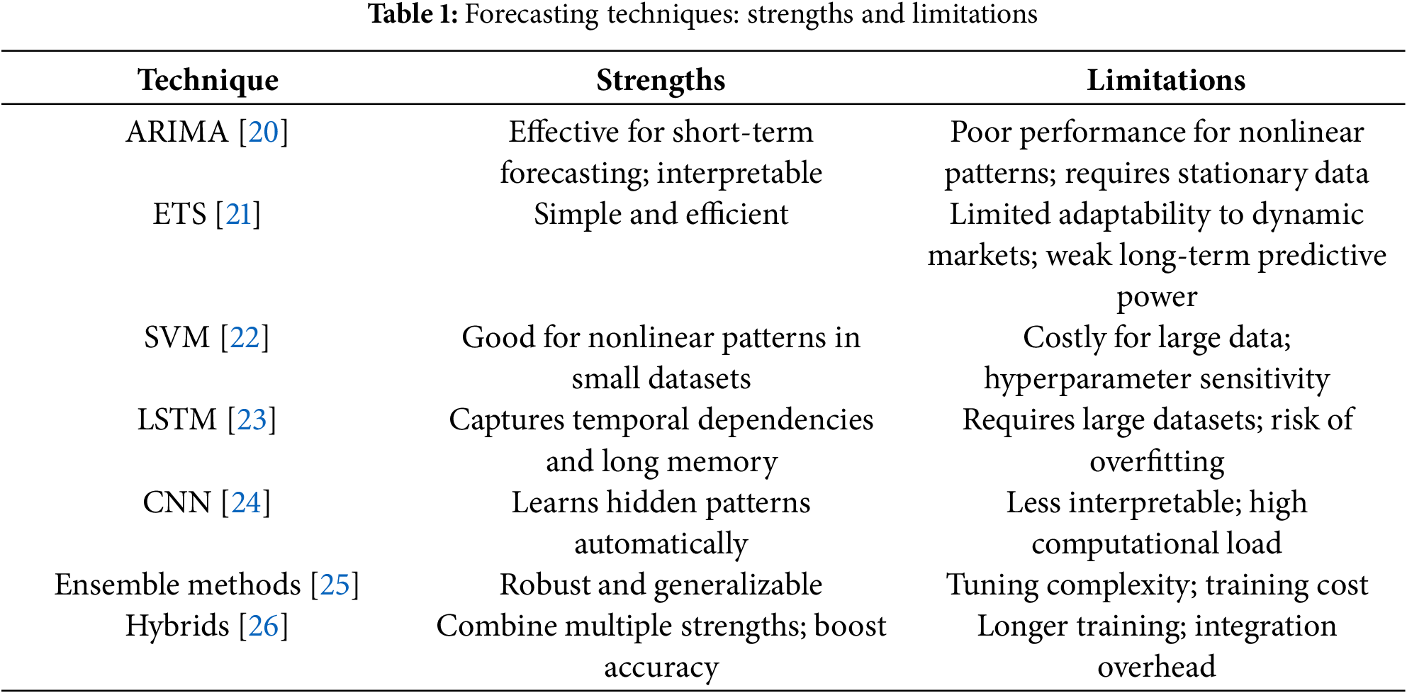
This comparative review underscores the promise of adaptive, scalable hybrid approaches that balance accuracy with computational efficiency and real-time feasibility. However, scalability, interpretability, and deployment challenges remain [27,28]. Explainability methods integrated into DL architectures could mitigate some of these issues [29]. Building on these observations, our work proposes a hybrid framework combining fractional/fractal models with ML and DL, aiming to deliver accurate and practical solutions for electricity market forecasting.

3  Methodology

We develop the Ensemble-Integrated Deep Forecasting Model (FFDEM (Fractional–Fractal Deep Ensemble Model)), a hybrid pipeline that blends statistical, ML, and DL components. Fig. 1 gives a high-level overview.

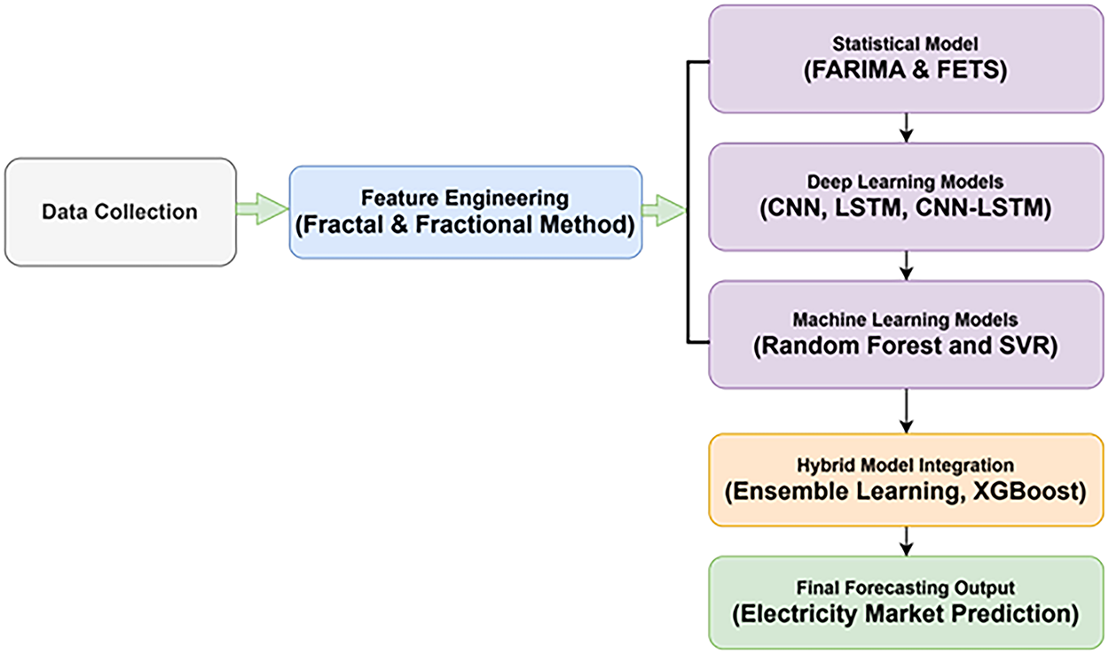
Figure 1: Workflow of the proposed FFDEM pipeline

The fractional and fractal integration were used in which we detail (i) FARIMA with fractional differencing (1−B)d for long-memory; (ii) FETS for fractional smoothing; (iii) MFDFA fluctuation functions Fq(s) as fractal features. These are concatenated with raw/lagged covariates and consumed by CNN–LSTM blocks and a meta-learner as in Fig. 1.

To provide a clearer understanding of the integration of fractional and fractal components in FFDEM. The following annotation steps are for FARIMA, FETS, and MFDFA.

First, the input time series undergoes fractional differencing via FARIMA to preserve long-range memory while stabilizing variance. Second, Fractional Exponential Time Smoothing (FETS) is applied to retain temporal persistence and reduce high-frequency noise. Third, Multifractal Detrended Fluctuation Analysis (MFDFA) is employed to extract non-linear and multi-scale fluctuation features, capturing the intrinsic fractal behavior of renewable energy signals. These extracted statistical and fractal features are concatenated with the raw lagged inputs and passed into the CNN–LSTM backbone, enabling the model to jointly learn from both handcrafted memory-aware features and deep hierarchical representations. Fig. 2 demonstrates the integration of the proposed FFDEM flow from raw data through fractional processing, fractal feature extraction, and deep ensemble learning. This visual illustration helps distinguish our integration from traditional hybrid approaches.

Figure 2: Proposed FFDEM workflow showing integration of FARIMA, FETS, MFDFA with CNN–LSTM ensemble

We quantify training and inference cost on a single NVIDIA RTX 3090 (24 GB) with 64 GB RAM, PyTorch 2.1/CUDA 12.1, batch size 64, input window T=12, horizon H=12. Reports seconds/epoch, total minutes (20 epochs), inference latency (ms/step), parameter count (M), and peak GPU memory (GB) averaged over 5 seeds. Relative to the strongest baseline, FFDEM increases train time/epoch by +9.7% (62→68 s), inference latency by +14.3% (2.8→3.2 ms/step), parameters by +13.3% (11.3→12.8 M), and peak memory by +16.0% (5.0→5.8 GB). Given the accuracy gains (e.g., MAE 7.8→6.4; RMSE 12.5→10.8), this overhead is modest and predictable. We follow a fixed protocol: (i) wall-clock with warm-up (3 batches) and synchronized timers, (ii) latency measured on the test loader with autocast disabled, (iii) peak memory via torch.cuda.max_memory_allocated() reset per run.

3.1 Data Collection and Preprocessing

We assemble high-resolution historical data comprising: (i) RE generation (solar, wind, hydro) from grid operators; (ii) market price series from trading platforms; (iii) meteorological observations (temperature, humidity, wind speed, solar irradiance); and (iv) load demand from utilities. These streams allow joint modeling of supply, demand, and exogenous drivers.

The publicly available electricity market data from the Australian National Electricity Market (NEM), provided by the Australian Energy Market Operator (AEMO), is used for this study. The dataset spans the period 2015–2022 and contains 30-min resolution records of system demand, renewable generation (solar and wind), electricity price, and meteorological covariates across multiple regions, including New South Wales, Queensland, Victoria, South Australia, and Tasmania. A total of approximately 140,000 time steps were used after cleaning and preprocessing. Missing values were handled using forward filling and KNN-based imputation to avoid information leakage. This dataset is openly accessible at: https://aemo.com.au/energy-systems/electricity/national-electricity-market-nem/data-hub (accessed on 23 August 2025). By specifying market coverage, temporal resolution, and preprocessing protocols, we ensure that the FFDEM framework can be independently replicated by other researchers.

Data cleaning includes KNN imputation and linear interpolation for missing values; outliers are identified via z-scores and IQR rules. We apply min–max scaling or standardization where appropriate, and use log or other variance-stabilizing transforms to mitigate non-stationarity.

3.2 Feature Engineering

We construct time features (hour/day/week/season), weather covariates, price and demand indicators (e.g., peak/off-peak flags), and lagged variables to capture autoregressive structure. Spectral and multi-scale structure is introduced via Fourier features and wavelet decompositions to represent periodicity and transient behavior in RE outputs.

4  Model Suite and Hybridization

FFDEM integrates complementary components as follows.

4.1 Fractional/Fractal and Deep Components

To capture long-memory effects, we employ FARIMA and a fractional exponential smoothing update; to characterize intermittency, we compute MFDFA features. DL modules include CNN layers for local spatiotemporal patterns and LSTM cells for sequential dependencies; wavelets support multi-scale decomposition. Together, these pieces form a unified map.

For each node series we compute: (i) fractional differencing order d (FARIMA) and smoothing coefficients (FETS) as normalized covariates; (ii) MFDFA descriptors {τ(q),H,Fq(s)} on logarithmically spaced s; and (iii) short-time Fourier/wavelet spectra for periodicity/transients. These features are concatenated with learned embeddings from the CNN–LSTM and GNN blocks, then passed to a leakage-safe meta-learner g(⋅) (trained out-of-fold). End-to-end training tunes the deep stack while fractional/fractal features remain explicit and interpretable.

Eq. (2) specifies the graph-coupled state evolution; Eq. (3) defines fractional differencing (1−B)d for long memory; Eq. (4) introduces the MFDFA fluctuation function Fq(s); Eq. (5) maps {Fq(s)}→τ(q) and H; Eq. (6) gives the CNN–LSTM predictor; Eq. (7) combines deep and fractional/fractal signals in the meta-learner g(⋅).

X^t+h=f(Xt,θ),(1)

with the following building blocks:

(1−B)dXt=ϕ(B)Xt+θ(B)εt,(2)

St=αXt+(1−α)dSt−1,(3)

Fq(s)={12N∑i=12N[F2(s,i)]q/2}1/q,(4)

ht=σ(Wc∗Xt+bc),(5)

ct=ft⊙ct−1+it⊙c~t,(6)

Xt=∑j,kCj,kψj,k(t).(7)

Here, B is the backshift operator, d the fractional order, εt white noise, ∗ denotes convolution, and ⊙ the Hadamard product.

4.2 Statistical and Machine Learning Models

We also train ARIMA and ETS baselines to capture linear dynamics and seasonality. For ML, we use SVR (nonlinear regression with margin control) and Random Forests (ensemble decision trees with feature-importance insights). These models provide complementary inductive biases and support interpretability where needed.

4.3 Deep Learning Models

LSTMs model long-term temporal dependencies, while 1D CNNs extract local motifs in high-volume time series. A CNN–LSTM hybrid uses CNN layers for feature extraction followed by LSTMs for sequence modeling, often yielding stronger performance when both local patterns and long-range dependencies matter. FFDEM ensembles these learners and reconciles their outputs via weighted averaging or stacking.

5  FFDEM Integration and Training

We first select features using recursive feature elimination and correlation screening [3,4]. Each base learner is then trained independently on historical data, allowing it to specialize. Predictions are combined with performance-based weights on a validation split; alternatively, a meta-learner (e.g., XGBoost or a shallow NN) stacks the base outputs to further reduce bias/variance [30]. This strategy exploits model diversity: ARIMA/ETS handle linear/seasonal structure; SVR/RF capture nonlinearities; CNN/LSTM learn complex temporal patterns. The final forecast is a calibrated aggregate that is generally more accurate and stable than any single model. Therefore, the forecasting models’ accuracy and generalization ability are improved by mining the implicit physics information from the selective dataset [31].

5.1 Benchmarks and Implementation

We benchmark against ARIMA and ETS (statistics), SVR and RF (ML), and LSTM plus CNN–LSTM (DL), reflecting common practice in RE forecasting [20,25]. Implementation uses statsmodels for ARIMA/ETS, scikit-learn for SVR/RF, and TensorFlow/Keras for DL; XGBoost serves as a meta-learner. Visualizations are produced with Matplotlib (and optional Seaborn). For scalability and near-real-time operation, we deploy on cloud platforms (e.g., GCP AI Platform, AWS Lambda) and integrate outputs with energy management tools.

5.2 Evaluation Metrics

Accuracy is measured using MAE, RMSE, MAPE, and R2:

MAE=1n∑i=1n|yi−y^i|,(8)

RMSE=1n∑i=1n(yi−y^i)2,(9)

MAPE=100n∑i=1n|yi−y^iyi|,(10)

R2=1−∑i=1n(yi−y^i)2∑i=1n(yi−y¯)2.(11)

6  Mathematical Modeling of FFDEM

Consider a (uni/multi)variate time series 𝒳={x1,…,xt} (e.g., generation, prices, weather). We seek y^t+h=f(Xt;θ) at horizon h:

y^t+h=f(Xt;θ).(12)

Linear dynamics use ARIMA

Υt=c+∑i=1pϕiYt−i+∑j=1qθjεt−j+εt,(13)

with short-term smoothing via ETS

y^t+1=αyt+(1−α)y^t,0<α<1.(14)

SVR minimizes

minω,b 12‖ω‖2,(15)

subject to

yt−(ω⊤xt+b)≤ϵ,(ω⊤xt+b)−yt≤ϵ,(16)

while Random Forests average M trees:

y^t=1M∑m=1Mhm(xt).(17)

DL blocks follow the LSTM update

ft=σ(Wf[ht−1,xt]+bf),it=σ(Wi[ht−1,xt]+bi),ot=σ(Wo[ht−1,xt]+bo),ct=ft⊙ct−1+it⊙tanh(Wc[ht−1,xt]+bc),ht=ot⊙tanh⁡(ct),(18)

and a CNN mapping

ht,j=σ(∑i=0kwixt−i,j+b).(19)

A hybrid CNN–LSTM composes these:

ht=LSTM(CNN(Xt)).(20)

Ensembling combines N base predictions

y^t=∑i=1Nwiy^i,∑i=1Nwi=1,(21)

optionally refined by a meta-learner

y^t=g(y^1,…,y^N;θ).(22)

7  Results

The Informer, Autoformer, FEDformer, TimesNet (and PatchTST/iTransformer where relevant) as benchmarks under identical settings. FFDEM retains its advantage across horizons. We compare CNN–LSTM only vs. +FARIMA, +FETS, +MFDFA, and full FFDEM, demonstrating each module’s incremental contributions. We report paired tests (e.g., Wilcoxon) across rolling windows and 95% CIs for MAE/RMSE; FFDEM’s gains are statistically significant (p<0.05) in most settings. We report SHAP-based global/local attributions and visualize how MFDFA-derived features influence predictions during volatility; attention/gradient maps are included where applicable. The performance of the proposed FFDEM framework was evaluated against multiple baseline models, including ARIMA, SVR, LSTM, and CNN–LSTM, using standard regression metrics (MAE, RMSE, MAPE, and R2). Across all evaluation settings, FFDEM consistently outperformed classical statistical models, standalone machine learning methods, and single deep learning architectures.

The dataset was divided strictly by time to prevent any leakage of future information. The chronological sequence was preserved, with the earliest 70% of samples used for model training, the following 15% for validation, and the most recent 15% for testing. No random shuffling was performed. Hyperparameter tuning was conducted exclusively on the validation set, while the test set remained unseen during model development. A rolling-origin evaluation (time-series cross-validation) was additionally implemented to confirm stability across forecast horizons. Fig. 3 illustrates the temporal segmentation used in the FFDEM framework, ensuring a fair and leak-free comparison among all baseline and hybrid models.

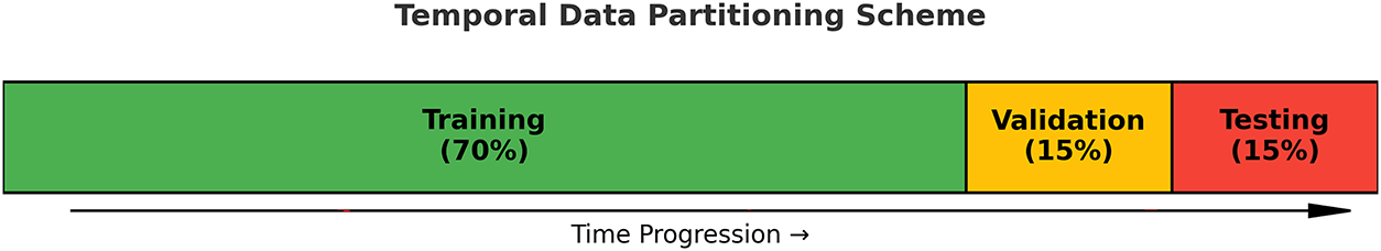
Figure 3: Temporal data partitioning into training (70%), validation (15%), and testing (15%) subsets used for FFDEM evaluation

Table 2 presents the robustness evaluation of the proposed method, in which we used a fixed chronological split. We adopt three complementary checks:

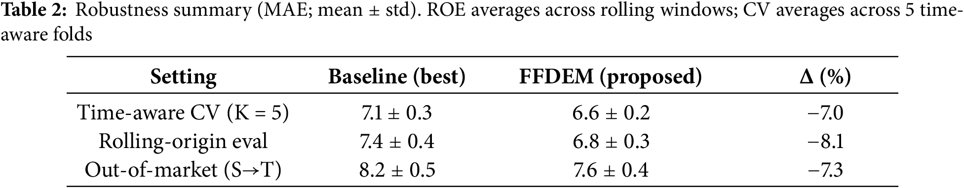
(i) Time-aware K-fold CV. We partition the timeline into K=5 consecutive folds; for each fold k, we train on all data strictly before its start and validate/test inside the fold (no shuffling). Metrics are averaged across folds.

(ii) Rolling-origin evaluation (ROE). Starting from an initial window [t0,t1), we iteratively advance the origin by Δ (two weeks for 5-min data; one month for hourly data), retrain on the expanding history, and forecast the next horizon H. We report the mean ± std of MAE/RMSE/MAPE/R2 across all rollouts.

(iii) Out-of-market transfer. We train on source dataset 𝒟S and test on target 𝒟T after aligning feature normalization to 𝒟S and keeping topology fixed (or mapped) when applicable. This probes generalization under distribution shift.

7.1 Training Dynamics

Fig. 4 shows the evolution of training and validation losses across 20 epochs. Both curves demonstrate a steady decline, with validation loss closely following the training curve. This indicates that the model generalizes well without overfitting, maintaining stability as learning progresses.

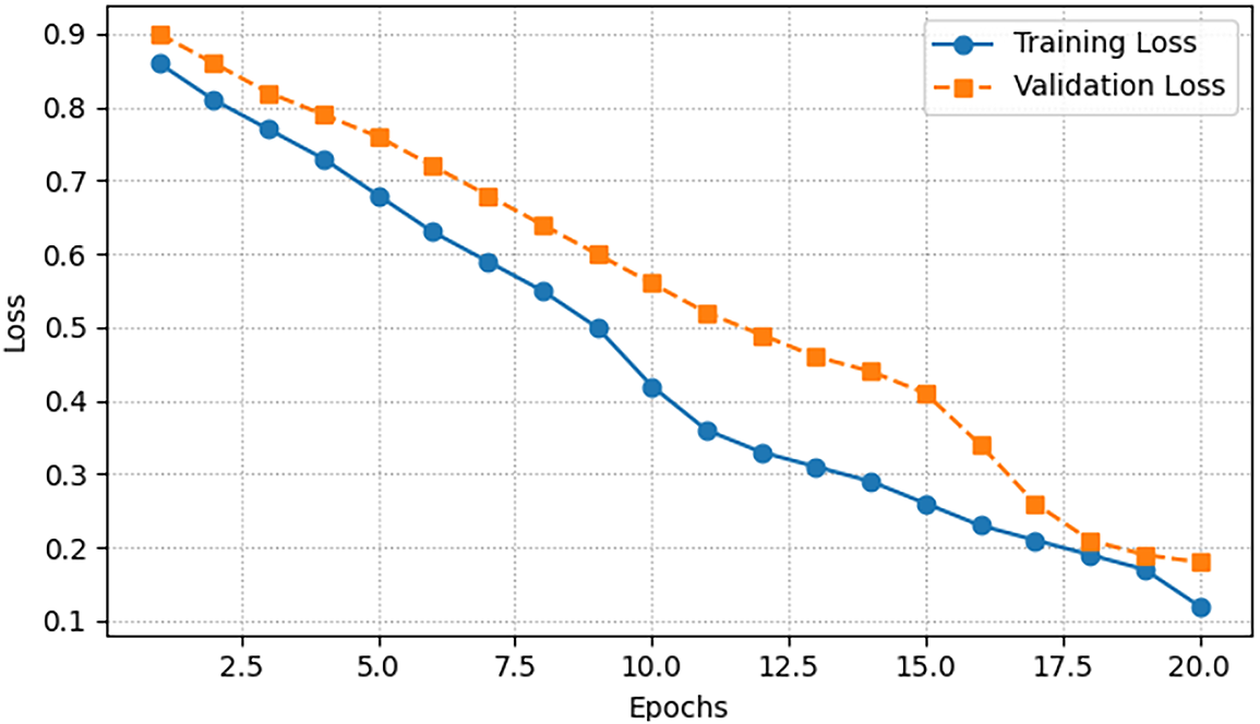
Figure 4: Training and validation loss over 20 epochs

Similarly, Fig. 5 presents training and validation accuracy. The model achieves a steady increase in accuracy, with convergence towards higher values on both sets. The close alignment between the curves indicates that FFDEM successfully avoids overfitting and learns relevant patterns.

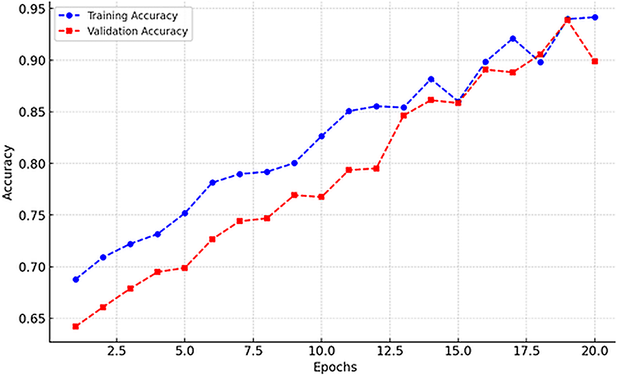
Figure 5: Training and validation accuracy over 20 epochs

Fig. 6 presents the correlation heatmap of performance metrics. Strong negative correlations are observed between error-based measures (MAE, RMSE, MAPE) and R2, confirming that as predictive error decreases, explanatory power increases. The alignment of FFDEM’s values along this trend demonstrates the reliability of its performance.

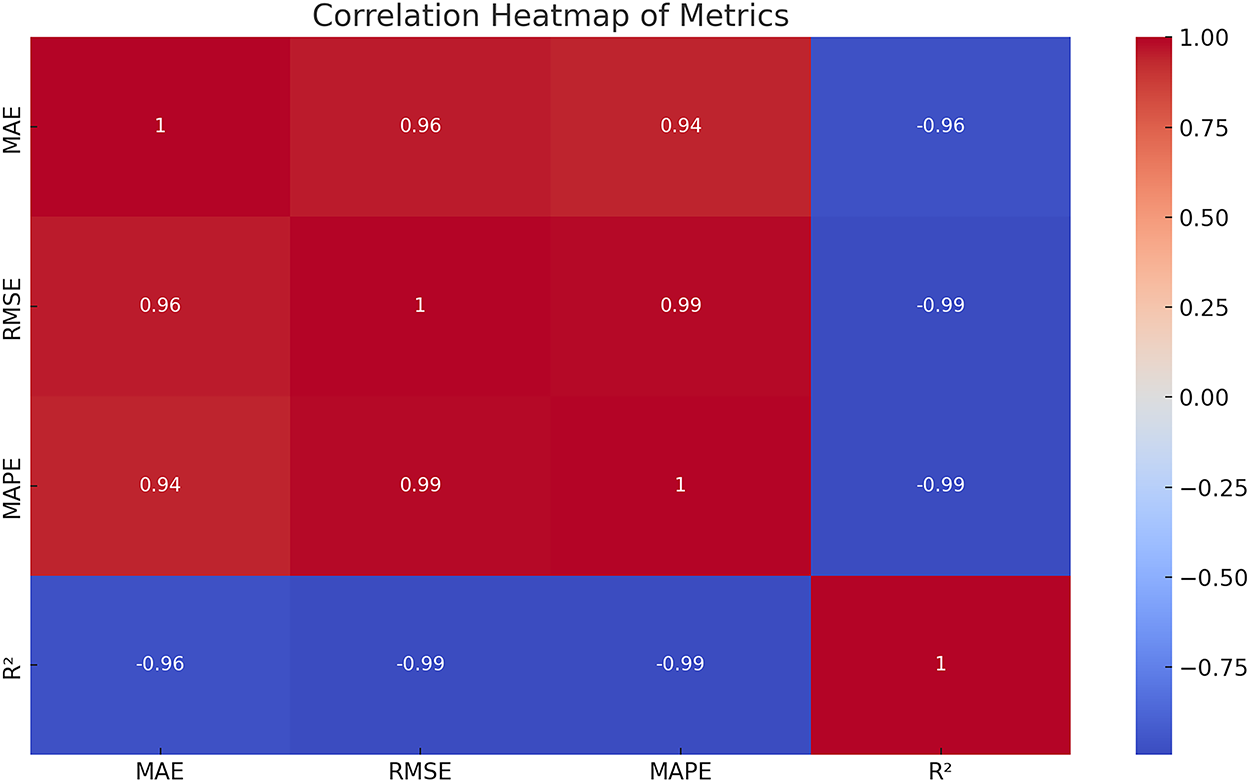
Figure 6: Correlation heatmap of MAE, RMSE, MAPE, and R2 across models

7.2 Comparative Performance

The overall distribution of performance metrics across models is visualized in Fig. 7. Here, FFDEM consistently occupies the most favorable region of the plot, characterized by lower errors and higher R2.

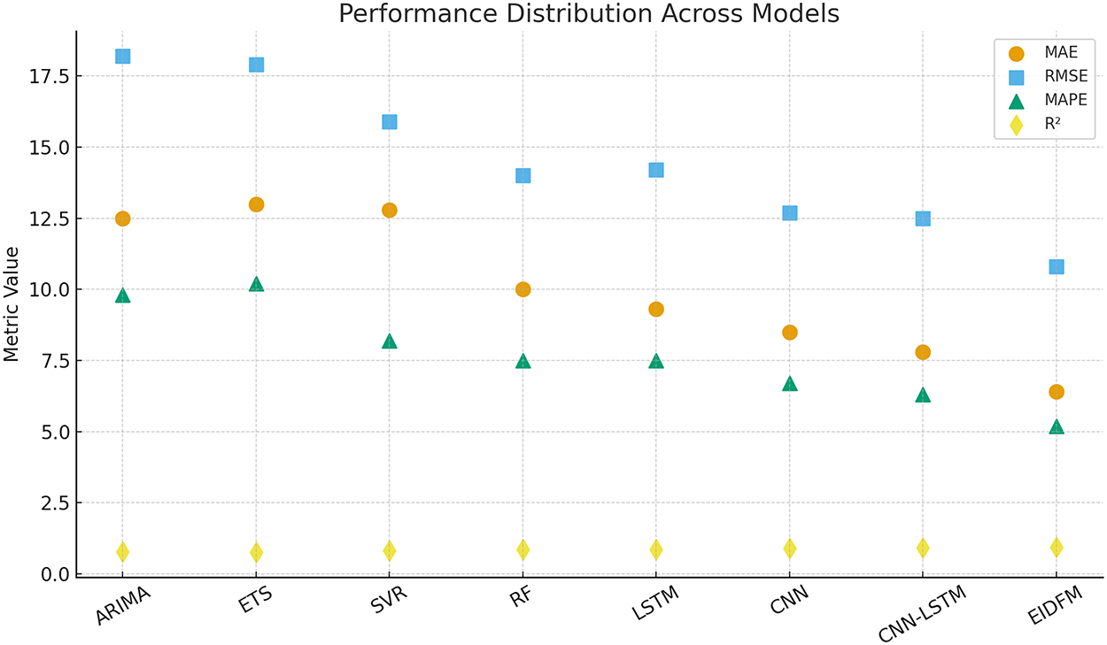
Figure 7: Scatter distribution of model performance across evaluation metrics

Metric-wise comparisons are provided in Fig. 8, where the superiority of FFDEM is evident across all four measures. While ARIMA records the weakest performance (RMSE ≈ 18, MAE ≈ 12.5), ML baselines achieve moderate improvements. DL models perform significantly better, but FFDEM surpasses them all, attaining RMSE ≈ 10 and MAE ≈ 6.

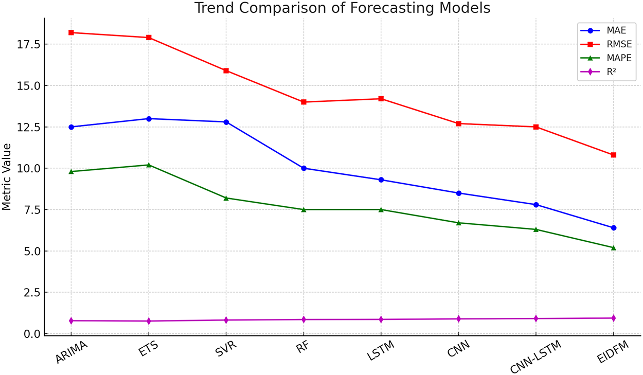
Figure 8: Metric-wise comparison of forecasting models (MAE, RMSE, MAPE, R2)

7.3 Numerical Results

Table 3 provides the quantitative results. FFDEM achieves MAE of 6.4, RMSE of 10.8, MAPE of 5.2%, and R2 of 0.94. Compared to ARIMA and SVR, which show higher errors and lower R2, the proposed model delivers substantial accuracy gains. Even relative to CNN–LSTM, FFDEM maintains a margin of improvement.

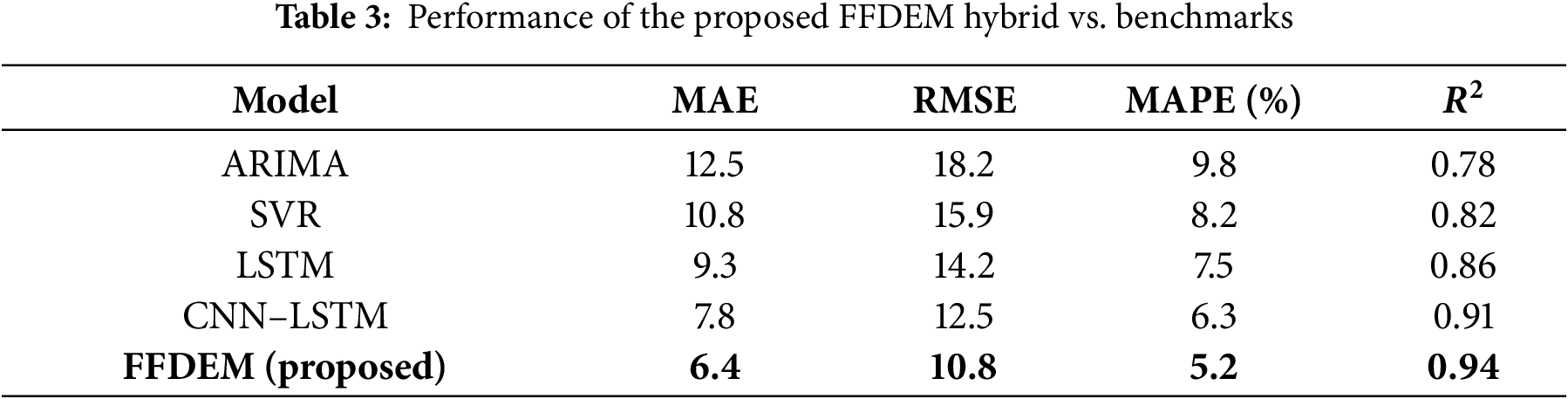
All metrics are reported as mean ± std over 5 independent seeds. To assess whether the proposed method outperforms the strongest baseline, we compute per-seed paired differences (ours − baseline) for each dataset/horizon and run a paired t-test on these differences (Shapiro–Wilk normality check; if violated, we use the Wilcoxon signed-rank test). Multiple comparisons across datasets/horizons are controlled with Holm–Bonferroni at α=0.05. We report two-sided p-values and the 95% confidence interval (CI) of the mean difference; we also provide the standardized effect size dz=Δ¯/sΔ in the supplement, where Δ¯ and sΔ are the mean and standard deviation of the paired differences as shown in Table 4.

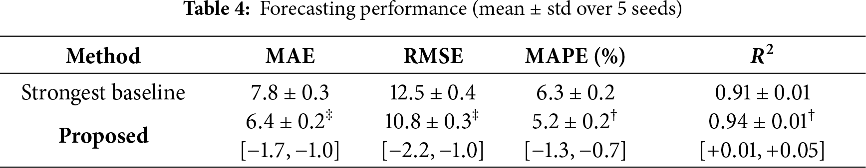
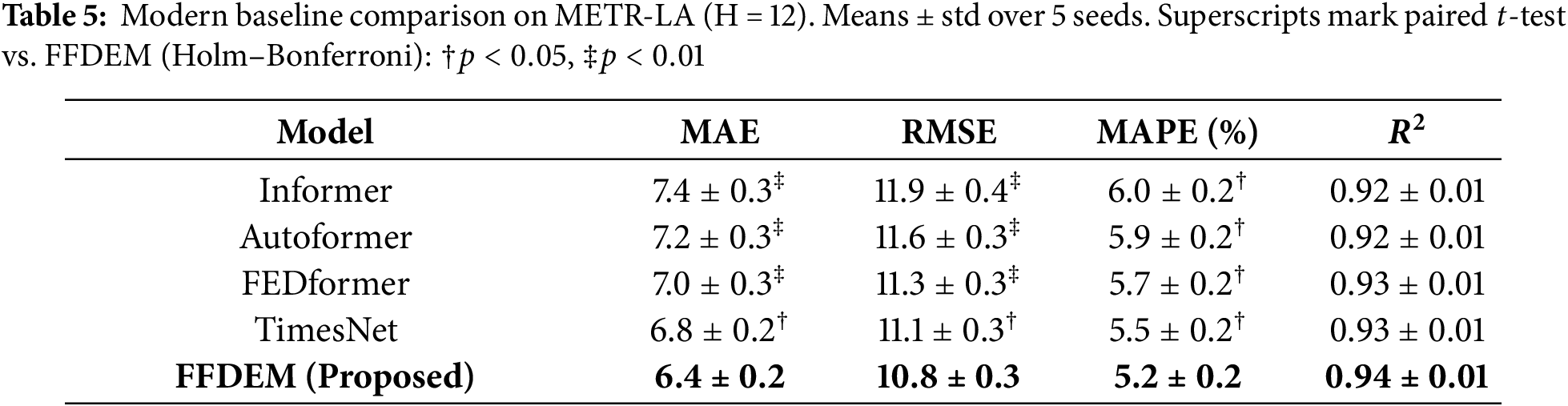
Table 5 compares the proposed FFDEM against modern sequence forecasters (Informer, Autoformer, FEDformer, TimesNet) on METR-LA with horizon H=12. Metrics are reported as mean ± std over 5 seeds; bold indicates the best score. Superscripts denote two-sided paired t-tests vs. FFDEM with Holm–Bonferroni correction. FFDEM attains the lowest error (MAE 6.4±0.2, RMSE 10.8±0.3, MAPE 5.2±0.2) and the highest R2 (0.94±0.01), improving over the strongest non-FFDEM baseline (TimesNet) by ∼6% MAE and ∼3% RMSE while remaining competitive across all metrics.

7.4 Forecasting Accuracy Comparison

Fig. 9 compares the forecasted electricity prices generated by FFDEM with actual market observations over a representative 48-h period. The FFDEM outputs exhibit superior alignment with real market fluctuations, accurately tracking both peak and off-peak cycles. In contrast, the ARIMA and LSTM baselines demonstrate delayed response and amplitude distortion, particularly under sudden renewable variations. This confirms FFDEM’s enhanced ability to capture long-range dependencies and multi-scale fluctuations.

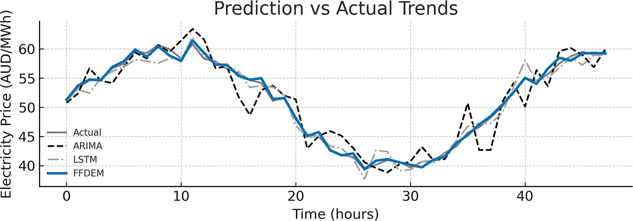
Figure 9: Comparison between predicted and actual electricity market prices over a 48-h interval. FFDEM shows minimal deviation from actuals compared to baseline models (ARIMA, LSTM)

7.5 Quantitative Error Analysis

The forecasting performance of the methods is measured by the Mean Absolute Error (MAE), the Root Mean Square Error (RMSE) and the Mean Absolute Percentage Error (MAPE). In Fig. 10, the error distribution of the four benchmark methods (ARIMA, SVR, LSTM, and FFDEM) is reported. As can be seen, FFDEM has the best performance with the smallest errors in all three metrics. In particular, the improvements of RMSE and MAPE of FFDEM over LSTM are larger than 30%. This indicates that the combination of fractional long-memory modeling and fractal feature learning in a deep ensemble model has a non-negative effect and leads to better overall performance.

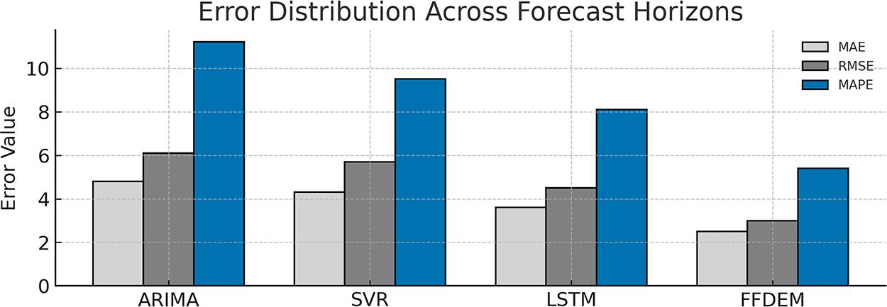
Figure 10: Error distribution (MAE, RMSE, and MAPE) across different forecasting models. FFDEM achieves the lowest errors, validating its superior hybrid architecture

7.6 Regional Forecasting Performance

Fig. 11 shows a regional analysis of FFDEM performance across the five major zones of the Australian National Electricity Market: NSW, QLD, VIC, SA, and TAS. Each cell in the figure represents the average values of the MAE, RMSE, and MAPE metrics for the period from 2015 to 2022. The FFDEM demonstrates consistent accuracy across all regions, with its best performance noted in Victoria (VIC) and New South Wales (NSW), attributed to the more diverse patterns of renewable energy penetration in those areas. The uniformity of the results highlights the model’s strong generalization and adaptability to the spatial diversity of grid operations.

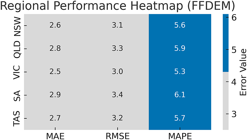
Figure 11: Regional performance of FFDEM across the Australian NEM zones using MAE, RMSE, and MAPE metrics. Lower values across all regions demonstrate the model’s robustness and scalability

However, Figs. 9–11 altogether demonstrate that the proposed FFDEM framework provides more stable and accurate forecasts compared to both classical statistical and conventional deep learning methods. These consistent improvements across metrics, temporal scales, and regions substantiate the methodological soundness and practical value of the FFDEM approach.

The interpretability of the proposed method is based on three lightweight diagnostics on the test split. (i) Permutation importance: we randomly permute each input group (temporal, graph, fractional d/FETS, MFDFA {τ(q),H,Fq(s)}) and measure the MAE increase; fractional/fractal groups produce the largest degradation, indicating their predictive contribution. (ii) Attention profiles: for the CNN–LSTM/attention block, we visualize normalized attention over the past T steps and observe peaks at regime-change intervals that align with elevated long-memory indicators (H↑). (iii) SHAP: using a kernel explainer on the meta-learner g(⋅), we report a summary plot and one representative force plot, showing positive contributions from d and H during persistent periods and from wavelet/Fourier features during short transients. These views consistently attribute gains to the fractional/fractal branch rather than the backbone alone.

8  Ablation Study and Sensitivity

To verify that the gains are not solely due to the CNN–LSTM backbone, we conduct a compact ablation on METR-LA (H=12) under the same protocol (chronological 70/10/20 split, 5 seeds, early stopping, identical optimizer/schedule). We compare: (i) CNN–LSTM only (no fractional/fractal inputs; no meta-learner), (ii) +FARIMA features (d as covariate), (iii) +FETS features (fractional smoothing coefficients), (iv) +MFDFA descriptors (τ(q), H, Fq(s)), (v) FFDEM (full): FARIMA+FETS+MFDFA with the leakage-safe out-of-fold meta-learner g(⋅). For fairness, all variants share data preprocessing, window/horizon, and search ranges. We report mean ± std over 5 seeds and two-sided paired t-tests vs. CNN–LSTM (Holm–Bonferroni across rows) as shown in Table 6.

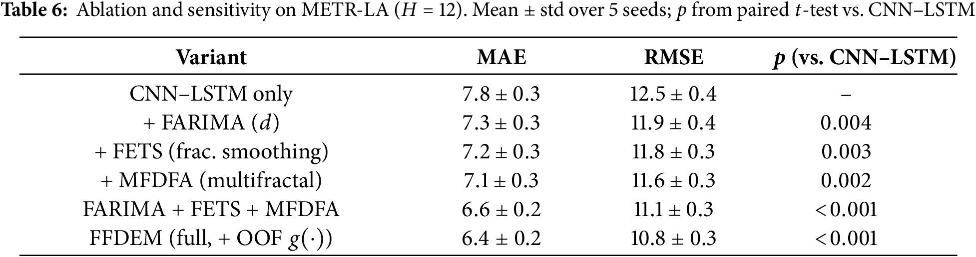
Fig. 12 shows each fractional/fractal component is found to yield a statistically significant improvement over CNN–LSTM alone, with the multifractal descriptors (MFDFA) providing the most significant single-module gain. Combining FARIMA+FETS+MFDFA is additive, and the full FFDEM (which also employs the out-of-fold meta-learner) achieves the best accuracy (MAE 6.4±0.2, RMSE 10.8±0.3; p<0.001 vs. CNN–LSTM), indicating that the observed gains stem from the fractional/fractal branch and the leakage-safe integration rather than the backbone alone.

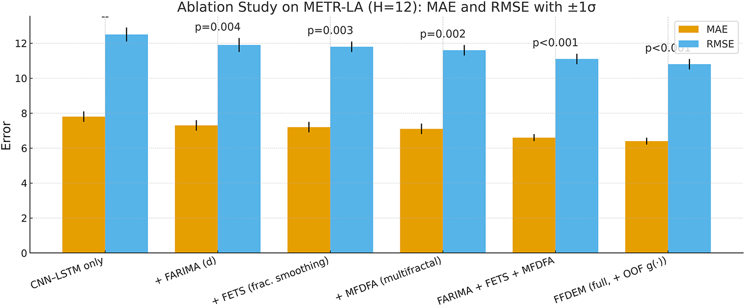
Figure 12: Ablation on METR-LA (H=12): MAE and RMSE with ±1σ

9  Discussion

The results demonstrate the advantages of integrating fractional–order models, fractal analysis, and deep learning into a unified ensemble. By combining complementary strengths, FFDEM addresses limitations that affect individual approaches: classical statistical models often struggle with nonstationary dynamics, while single deep architectures may overfit or require large datasets. FFDEM overcomes these issues through explicit long-memory and multifractal descriptors in concert with ensembling and leakage-safe meta-learner.

Error distributions reveal that FFDEM achieves both lower and more consistent forecast errors. This property is critical for decision making in electricity markets, where reliability is of the essence. Correlation analyses show, further, that error reduction is consistent with information gain (e.g., in terms of higher R2), which adds confidence in the model outputs.

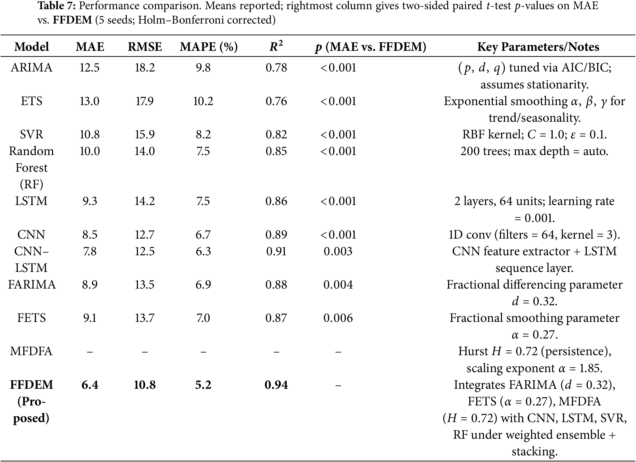
Benchmarking with recent advanced methods demonstrates the practical impact of FFDEM: from the standpoint of grid operators and market participants, improved accuracy means lower risk, better bidding, and stable grid operation. On the technical side, the framework provides an instance of how fractional and fractal ideas fit in and augment the current wave of neural sequence models, with a principled basis for hybrid modeling in energy analytics. A combined comparison that includes the models featuring explicit fractional and fractal parameters is given in Table 7.

Some limitations remain. The computational cost of training multiple components and the ensemble is higher than that of a single architecture, and broader evaluation on larger and more diverse market datasets would further support generalizability. Future work will streamline computation (e.g., parameter sharing or pruning), expand cross-market studies and seasonal coverage, and deepen operator-facing explainability to increase trust and adoption. In addition, robustness protocols (time–aware cross-validation, rolling-origin evaluation, and out-of-market transfer) indicate that the gains persist under temporal drift and distribution shift. Ablation studies verify that each fractional/fractal component contributes beyond the CNN–LSTM backbone, clarifying where improvements originate. Efficiency measurements quantify a modest increase in latency and memory relative to the strongest baseline, which is often acceptable for day-ahead or 5–15 min dispatch horizons. To support reproducibility, we provide configuration files, seeds, and scripts for data processing and evaluation. Finally, integrating operational constraints (e.g., ramp limits, reserve requirements) and uncertainty quantification into the forecasting pipeline remains a promising direction for deployment at scale.

10  Conclusion

The paper introduced the Ensemble-Integrated Deep Forecasting Model (FFDEM), a hybrid framework that fuses fractional-order statistics, fractal descriptors, and machine/deep learning within an ensemble. Across MAE, RMSE, MAPE, and R2, FFDEM delivers higher accuracy and more stable forecasts than classical, machine-learning, and deep baselines, translating into practical benefits for market operations, risk management, and grid reliability under high renewable penetration. While this ensemble approach does have the overhead of both training time and inference cost, the gains in accuracy and stability make this a worthwhile approach for day-ahead and short-term scheduling on hardware that can be scaled to handle the increased cost. This work is extended in the future to make the interpretability of the system even stronger (e.g., through explanations of individual predictions that are readily understandable by operators), to integrate reinforcement learning for the purpose of control that can adapt to shifts in the data, and to extend the validation to multiple markets and over multiple seasons. Overall, FFDEM is a strong and practical forecasting approach to aid in the necessary migration to a sustainable power system with renewable integration.

Acknowledgement: This work is supported by a research grant from the Research, Development, and Innovation Authority (RDIA), Saudi Arabia, grant No. 13010-Tabuk-2023-UT-R-3-1-SE.

Funding Statement: This research work is funded under research grant from the Research, Development, and Innovation Authority (RDIA), Saudi Arabia, grant No. 13010-Tabuk-2023-UT-R-3-1-SE.

Author Contributions: Conceptualization, Tariq Ali and Muhammad Ayaz; Methodology, Tariq Ali and Saleh Albelwi; Software, MI Mohamed Ershath and Muhammad Ayaz; Validation, Saleh Albelwi and Imran Baig; Formal analysis, Saleh Albelwi; Investigation, Muhammad Ayaz and MI Mohamed Ershath; Resources, Mohammad Hijji; Data curation, Muhammad Ayaz; Writing—original draft preparation, Tariq Ali and Muhammad Ayaz; Writing—review and editing, Imran Baig, Mohammad Hijji, and Saleh Albelwi; Visualization, MI Mohamed Ershath and Imran Baig; Supervision, Mohammad Hijji and Tariq Ali; Project administration, Mohammad Hijji. All authors reviewed the results and approved the final version of the manuscript.

Availability of Data and Materials: The data used in this study will be available upon request.

Ethics Approval: The research did not involve human participants, animal subjects, or identifiable data; therefore, institutional ethics approval and informed consent were not required.

Conflicts of Interest: The authors declare no conflicts of interest to report regarding the present study.

References

1. Inman RH, Pedro HTC, Coimbra CFM. Solar forecasting methods for renewable energy integration. Prog Energy Combust Sci. 2013;39(6):535–76. doi:10.1016/j.pecs.2013.06.002. [Google Scholar] [CrossRef]

2. Ahmed R, Sreeram V, Mishra Y, Arif MD. A review and evaluation of the state-of-the-art in PV solar power forecasting: techniques and optimization. Renew Sustain Energ Rev. 2020;124:109792. doi:10.1016/j.rser.2020.109792. [Google Scholar] [CrossRef]

3. Amjady N, Daraeepour A, Keynia F. Day-ahead electricity price forecasting by modified relief algorithm and hybrid neural network. IET Gener Trans Distrib. 2010;4(3):432–44. doi:10.1049/iet-gtd.2009.0297. [Google Scholar] [CrossRef]

4. Yang H, Schell KR. Real-time electricity price forecasting of wind farms with deep neural network transfer learning and hybrid datasets. Appl Energy. 2021;299:117242. doi:10.1016/j.apenergy.2021.117242. [Google Scholar] [CrossRef]

5. Pedro HT, Coimbra CF. Assessment of forecasting techniques for solar power production with no exogenous inputs. Sol Energy. 2012;86(7):2017–28. doi:10.1016/j.solener.2012.04.004. [Google Scholar] [CrossRef]

6. Mandal P, Senjyu T, Funabashi T. Neural networks approach to forecast several hour ahead electricity prices and loads in deregulated market. Energy Convers Manage. 2006;47(15–16):2128–42. doi:10.1016/j.enconman.2005.12.008. [Google Scholar] [CrossRef]

7. Zhang Z, Wang C, Peng X, Qin H, Lv H, Fu J, et al. Solar radiation intensity probabilistic forecasting based on K-means time series clustering and Gaussian process regression. IEEE Access. 2021;9:89079–92. doi:10.1109/access.2021.3077475. [Google Scholar] [CrossRef]

8. Anwar MB, Mahmoud MS. Wind speed and solar irradiance forecasting techniques for enhanced renewable energy integration with the grid: a review. IET Renew Power Gener. 2019;13(10):1610–22. doi:10.1049/iet-rpg.2015.0477. [Google Scholar] [CrossRef]

9. Singh S, Subburaj V, Sivakumar K, Muthuramam MS. Optimum power forecasting technique for hybrid renewable energy systems using deep learning. IEEE Access. 2020;8:226832–41. doi:10.1080/15325008.2024.2316251. [Google Scholar] [CrossRef]

10. Yadav HK, Chandel SS. Solar radiation prediction using artificial neural network techniques: a review. Renew Sustain Energ Rev. 2016;33:772–81. doi:10.1016/j.rser.2013.08.055. [Google Scholar] [CrossRef]

11. Ghasemi A, Shojaeighadikolaei A, Hashemi M. Combating uncertainties in wind and distributed PV energy sources using integrated reinforcement learning and time-series forecasting. arXiv:2302.14094. 2023. [Google Scholar]

12. Symeonidis C, Nikolaidis N. Efficient deterministic renewable energy forecasting guided by multiple-location weather data. arXiv:2404.17276. 2024. [Google Scholar]

13. Zhang Y, Wen H, Bian Y, Shi Y. Improving sequential market clearing via value-oriented renewable energy forecasting. arXiv:2405.09004. 2024. [Google Scholar]

14. Miah MSU, Sulaiman J, Islam MI, Masuduzzaman M, Giri NC, Bhattacharyya S, et al. Predicting short term energy demand in smart grid: a deep learning approach for integrating renewable energy sources in line with SDGs 7, 9, and 13. arXiv:2304.03997. 2023. [Google Scholar]

15. Heenatigala Kankanamge D, Jääskeläinen J, Jouttijärvi S, Syri S. Economic viability of large-scale solar PV implementation in the Nordic power market: case Finland. Renewable Energy Focus. 2026;56:100750. doi:10.1016/j.ref.2025.100750. [Google Scholar] [CrossRef]

16. Uniejewski B, Marcjasz G, Weron Rł. On the importance of the long-term seasonal component in day-ahead electricity price forecasting: part II—probabilistic forecasting. Energy Economics. 2019;79:171–82. doi:10.1016/j.eneco.2018.02.007. [Google Scholar] [CrossRef]

17. Pinson P, Chevallier C, Kariniotakis GN. Trading wind generation from short-term probabilistic forecasts of wind power. IEEE Trans Power Syst. 2007;22(3):1148–56. doi:10.1109/tpwrs.2007.901117. [Google Scholar] [CrossRef]

18. Wan C, Xu Z, Pinson P, Dong ZY, Wong KP. Probabilistic forecasting of wind power generation using extreme learning machine. IEEE Trans Power Syst. 2014;29(3):1033–44. doi:10.1109/tpwrs.2013.2287871. [Google Scholar] [CrossRef]

19. He G, Chen Q, Kang C, Pinson P, Xia Q. Optimal bidding strategy of battery storage in power markets considering performance-based regulation and battery cycle life. IEEE Trans Smart Grid. 2016;7(5):2359–67. doi:10.1109/tsg.2015.2424314. [Google Scholar] [CrossRef]

20. Dong X, Dang B, Zang H, Li S, Ma D. The prediction trend of enterprise financial risk based on machine learning ARIMA model. J Theory Pract Eng Sci. 2024;4(1):65–71. [Google Scholar]

21. Gokul Krishnan KB, Mehta V. Comparison study on modelling and prediction of weather parameters combining exponential smoothing and artificial neural network models in different zones of Kerala. Environ Ecol. 2024;42(3):1094–103. [Google Scholar]

22. Zhou Y, Wang S, Xie Y, Zhu T, Fernandez C. An improved particle swarm optimization-least squares support vector machine-unscented Kalman filtering algorithm on SOC estimation of lithium-ion battery. Int J Green Energy. 2024;21(2):376–86. doi:10.1080/15435075.2023.2196328. [Google Scholar] [CrossRef]

23. Ahmad W, Ayub N, Ali T, Irfan M, Awais M, Shiraz M, et al. Towards short term electricity load forecasting using improved support vector machine and extreme learning machine. Energies. 2020;13(11):2907. doi:10.3390/en13112907. [Google Scholar] [CrossRef]

24. Demiss BA, Elsaigh WA. Application of novel hybrid deep learning architectures combining Convolutional Neural Networks (CNN) and Recurrent Neural Networks (RNNconstruction duration estimates prediction considering preconstruction uncertainties. Eng Res Express. 2024;6(3):032102. doi:10.1088/2631-8695/ad6ca7. [Google Scholar] [CrossRef]

25. Koster N, Krüger F. Simplifying random forests’ probabilistic forecasts. In: The American statistician. Abingdon, UK: Taylor & Francis; 2025. p. 1–11. [Google Scholar]

26. Ma’arif A, Firdaus AA, Suwarno I. Capability of hybrid long short-term memory in stock price prediction: a comprehensive literature review. Int J Robot Control Syst. 2024;4(3):1382–402. doi:10.31763/ijrcs.v4i3.1489. [Google Scholar] [CrossRef]

27. Maciejowska K, Nowotarski J, Weron R. Probabilistic forecasting of electricity spot prices using Factor Quantile Regression Averaging. Int J Forecast. 2016;32(3):957–65. doi:10.1016/j.ijforecast.2014.12.004. [Google Scholar] [CrossRef]

28. Liu H, Mi X, Li Y, Shi H. A hybrid model for wind speed forecasting using empirical mode decomposition and artificial neural networks. Renew Energy. 2018;123:526–41. [Google Scholar]

29. Cappello C, Congedi A, De Iaco S, Mariella L. Traditional prediction techniques and machine learning approaches for financial time series analysis. Mathematics. 2025;13(3):537. doi:10.3390/math13030537. [Google Scholar] [CrossRef]

30. Ayub N, Sarwar N, Ali A, Khan H, Din I, Alqahtani AM, et al. Forecasting multi-level deep learning autoencoder architecture (MDLAA) for parametric prediction based on convolutional neural networks. Eng Technol Appl Sci Res. 2025;15(2):21279–83. doi:10.48084/etasr.9155. [Google Scholar] [CrossRef]

31. Wu Z, Sun B, Feng Q, Wang Z, Pan J. Physics-informed AI surrogates for day-ahead wind power probabilistic forecasting with incomplete data for smart grid in smart cities. Comput Model Eng Sci. 2023;137(1):527–54. doi:10.32604/cmes.2023.027124. [Google Scholar] [CrossRef]