
 Submit a Paper
 Propose a Special lssue
 Open Access
REVIEW
Advances in the Improved Element-Free Galerkin Methods: A Comprehensive Review
1 School of Applied Science, Taiyuan University of Science and Technology, Taiyuan, 030024, China
2 Shanghai Key Laboratory of Mechanics in Energy Engineering, Shanghai Institute of Applied Mathematics and Mechanics, School of Mechanics and Engineering Science, Shanghai University, Shanghai, 200072, China
* Corresponding Author: Yumin Cheng. Email:
Computer Modeling in Engineering & Sciences 2025, 145(3), 2853-2894. https://doi.org/10.32604/cmes.2025.073178
Received 12 September 2025; Accepted 20 November 2025; Issue published 23 December 2025
 View Full Text
 Download PDF
Abstract
The element-free Galerkin (EFG) method, which constructs shape functions via moving least squares (MLS) approximation, represents a fundamental and widely studied meshless method in numerical computation. Although it achieves high computational accuracy, the shape functions are more complex than those in the conventional finite element method (FEM), resulting in great computational requirements. Therefore, improving the computational efficiency of the EFG method represents an important research direction. This paper systematically reviews significant contributions from domestic and international scholars in advancing the EFG method. Including the improved element-free Galerkin (IEFG) method, various interpolating EFG methods, four distinct complex variable EFG methods, and a series of dimension splitting meshless methods. In the numerical examples, the effectiveness and efficiency of the three methods are validated by analyzing the solutions of the IEFG method for 3D steady-state anisotropic heat conduction, 3D elastoplasticity, and large deformation problems, as well as the performance of two-dimensional splitting meshless methods in solving the 3D Helmholtz equation.Keywords
As an important numerical computation method, the meshless (or meshfree) method operates solely on discrete points rather than predefined meshes. Consequently, it eliminates the need for remeshing when solving large deformation problems where mesh distortion typically occurs. This inherent advantage over the conventional finite element method (FEM) [1] has led to its widespread adoption across multiple scientific and engineering disciplines.
The development of the meshfree method originated in 1977 when Lucy pioneered the smoothed particle hydrodynamics (SPH) method [2], representing the first meshless computational method. Later in 1981, Lancaster and Salkauskas first proposed the moving least squares (MLS) approximation [3] for surface fitting applications. Building on this foundation, Nayroles et al. developed the diffuse element method (DEM) [4] in 1992, implementing MLS approximation for nodal approximation. Subsequently, in 1994, Belytschko et al. developed the element-free Galerkin (EFG) method [5], which also utilized MLS approximation with Lagrange multipliers for boundary condition enforcement. Since then, numerous other meshless methods have been proposed, including the reproducing kernel particle method (RKPM) [6], the finite point method [7], the partition of unity method [8], the radial basis function method [9], the boundary node method [10], the natural element method [11], the local Petrov-Galerkin method [12], the local boundary integral equation [13], the point interpolation method [14], the collocation meshless method [15], the hybrid boundary node method [16], the moving Kriging interpolation method [17], the meshless finite element method [18].
Among the various meshless methods, the EFG method proposed by Belytschko et al. [5] represents a fundamental and widely studied method in numerical computation. After the strong form of the governing differential equation is transformed into its weak integral form, and the shape function is introduced to derive the discrete equations, which are solved by using the computational tool of background integration mesh, ultimately yielding the numerical solution for the corresponding problem. The EFG method constructs shape functions using the MLS approximation [4], with error estimates analyzed by Li [19]. Noted for its foundation in least squares mathematical theory, the MLS approximation achieves high computational accuracy. A key advantage of the MLS method over the least squares method is its mobility and compact support. This allows for the use of a linear basis function to obtain stable and highly accurate numerical solutions. Currently, the EFG method has been applied to solve diverse problems, including transient heat transfer problem [20], hyperbolic problem [21], fracture mechanics [22,23], optimization design [24], dynamic boundary flow [25], magneto-electro-elastic plates [26], shrinkage analysis of round billets [27], free vibration of rotating nanobeams [28], wave propagation [29], Signorini-Tresca contact problem [30], topology optimization [31–33], free vibration [34], buckling [35] and nonlinear analyses [36,37]. Additionally, the coupled FEM-EFG method [38,39], the variational multiscale EFG method [40,41] and the enrichment of EFG method [42] have also been developed. However, the computation of the shape function in the EFG method demands significant computational resources, resulting in reduced efficiency. Additionally, it may encounter singular matrices during numerical implementation. These limitations necessitate further methodological improvements.
In 2003, Cheng and Chen [43] proposed the improved moving least squares (IMLS) approximation by replacing the basis function in MLS with orthogonal ones, resulting in higher computational efficiency. Later, in 2008, Zhang et al. studied the improved element-free Galerkin (IEFG) method based on the IMLS approximation and applied it to analyze 2D fracture problems. Subsequently, the IEFG method is successfully extended to solve various problems, including elasticity, potential problems [44,45], wave equation, heat conduction [46] and elastic dynamics problems. Cheng and Liew further applied the IEFG method to study the modified equal width (MEW) wave equation [47] and generalized Camassa and Holm equation [48]. Cheng et al. made significant contributions to advancing the IEFG method, applying it to problems such as the Schrödinger equation, viscoelasticity [49], fracture mechanics, topology optimization, elastoplasticity, and diffusional drug release [50] problems. Cheng et al. further integrated deep learning with the IEFG method for solving inverse potential problems [51]. Zhang et al. investigated the biological population problem using the IEFG method [52], while Li et al. conducted error analysis for the IEFG method [53] and later applied it to the elliptic problem [54], p-Laplacian problem [55], and Boussinesq equation [56]. Debbabi and BelhadjSalah selected the IEFG method for the thermo-elastic problem [57]. Mousavi et al. coupled it with the finite strip method to analyze plate vibration [58]. Guo et al. further extended its application to study vibration [59], nonlinear behavior [60], and flutter [61] in composite quadrilateral plates, in addition to the dynamics of cantilever plates [62]. The IEFG method offers the advantage of fast computational speed, effectively addressing the limitations of the EFG method, such as slow computation and the tendency to form singular matrices.
The shape functions in both EFG and IEFG methods lack interpolation properties, traditionally requiring the penalty method to impose the essential boundary conditions, which inevitably reduces computational efficiency. To address this limitation, Lancaster and Salkauskas proposed the interpolating MLS approximation [3], enabling direct imposition of Dirichlet boundary conditions without auxiliary methods. Ren et al. further simplified the derivation of the shape function and proposed the improved interpolating MLS approximation [63]. Wang and Sun analyzed its error estimates [64], while Li and Wang investigated its inherent instability [65]. By constructing shape function with this method, the improved boundary EFG method was proposed. Later, Ren et al. presented the interpolating EFG method for 2D elasticity [66], potential and heat conduction [67,68] problems. Liu and Cheng extended their application to study two-point boundary value, potential [69], heat conduction, elastoplasticity and large deformation [70] problems. Sun and Wang adopted the method for the regularized long wave equation [71]. Zhang and Peng applied it to the viscoelasticity problem [72]. Dehghan and Abbaszadeh solved the magnetohydrodynamics equation using the interpolating EFG method [73]. Shen et al. employed it for evolutionary variational inequalities [74] and the mixed complementarity problem [75]. Finally, Zhang and Li developed the variational multiscale interpolating EFG method [76,77] based on the improved interpolating MLS approximation [63]. Since the interpolating EFG method can directly impose boundary conditions like FEM and features a simpler formulation than the standard EFG method, it offers improved computational efficiency for solving scientific and engineering problems.
A limitation of the improved interpolating MLS method is that its weight function becomes singular at nodes, which inevitably introduces truncation errors. To overcome this issue, Wang et al. studied a novel interpolating MLS approximation [78] by replacing the singular weight function with the nonsingular alternative, subsequently developing the new interpolating EFG method [78]. Later, Sun et al. extended this method to solve elasticity [79] and elastoplasticity [80] problems. Dehghan et al. applied this method to diverse problems, including solutions for fractional diffusion-wave [81], inverse tempered fractional diffusion equations [82], and Oldroyd models [83], with additional contributions to decomposition variational multiscale interpolating EFG method [84]. Liu and Cheng further advanced the method for 2D large deformation analysis [85,86] and 3D elastoplasticity simulations [87]. Additionally, the interpolating boundary EFG method [88,89], variational multiscale interpolating EFG method [90], interpolating EFG scaled boundary method [91–93], coupled interpolating EFG method [94], regularized and adaptive orthogonal interpolating MLS approximation [95,96] were also developed by researchers. The interpolating meshless method based on non-singular weight functions offers a wide range of weight function options and overcomes the limitations associated with singular weight functions.
In 2022, Ma et al. combined the Hermite interpolation with MLS approximation to approximate the field variables, and then proposed the Hermite interpolation EFG method for solving the elasticity problem [97], functionally graded structures [98], piezoelectric materials [99], and functionally graded piezoelectric structures [100]. Its distinct advantage lies in providing superior accuracy for calculating function derivatives at any point within the solution domain. This stems from explicitly incorporating the normal derivatives of field functions during shape function construction, which is the distinctive feature absent in previous EFG improvements.
The EFG, IEFG, and three interpolation EFG methods all use scalar basis functions to establish shape functions. To reduce the number of undetermined coefficients in the shape function, Cheng and Li integrated the complex variable theory combined with the MLS approximation, developing the complex variable moving least squares (CVMLS) approximation. This innovation led to the complex variable element-free Galerkin (CVEFG) method [101] for solving elasticity problems. Typically, a linear basis function is selected for shape function construction. When a scalar basis is selected, the number of undetermined coefficients is three, which reduces to two for a vector basis function, thereby lowering the matrix order in the shape function computation.
The CVMLS approximation exhibits a minor limitation in that the mathematical and physical interpretation of its functional construction remains unclear. To address this issue, Bai et al. studied the improved complex variable moving least squares (ICVMLS) approximation [102] by replacing the basis function in the CVMLS approximation with a conjugate basis function. Subsequently, the improved complex variable element-free Galerkin (ICVEFG) method was successfully applied to solve a wide range of 2D problems including: elasticity [102], potential, advection-diffusion, Schrödinger, wave propagation, viscoelasticity [103], elastoplasticity, topology optimization [104], large deformation [105,106], as well as the bending problems of Kirchhoff plate and thin plate on elastic foundations [107]. Li and Tian further extended the ICVEFG method to large deformation [108–110] and fracture [111–113] problems. Li and Li conducted error estimation analyses for both the ICVMLS approximation and the ICVEFG method [114]. Additionally, Niu et al. integrated the conjugate basis function into the RKPM for solving the 2D elasticity problem [115]. However, the studies on the ICVEFG method in the aforementioned literature are confined to two-dimensional problems. To extend its applicability, Li and Li derived the 3D shape function calculation formula for CVMLS approximation [116], and Li subsequently developed the CVEFG method [117] for analyzing 3D partial differential equations. More recently, Yang et al. applied this method to solve 3D elastoplastic mechanics problems [118], thereby significantly expanding its scope of applicability.
The CVEFG and ICVEFG methods lack interpolation properties. Ren et al. addressed this limitation by developing the interpolating CVMLS approximation [119] through the incorporation of singular weight functions into the CVMLS framework. Building on this advancement, Deng and He successfully implemented the interpolating CVEFG method for temperature field analysis, and subsequently enhanced the approach by proposing an improved interpolating CVEFG method [120–124] by integrating the singular weight functions with ICVEFG approximations. This method addresses the inability of the ICVEFG method to directly apply boundary conditions and achieves improved computational efficiency.
Regardless of which of the aforementioned improved methods is employed, the influence domain of a point in 3D problems still constitutes a three-dimensional region. The number of points included within this domain is significantly larger than that in a 2D problem. Furthermore, shape functions must be computed for every point within the influence domain. As a result, the improvement in computational speed of the EFG method remains relatively constrained, particularly for 3D problems.
In 2017, Cheng et al. pioneered the integration of the dimension split method [125,126] with the ICVEFG method, leading to the development of the dimension splitting complex variable element-free Galerkin (DS-CVEFG) method [127]. This innovative approach demonstrated significant computational time savings compared to the IEFG method for solving 3D partial differential equations. The method operates by reducing the 3D problem to a series of 2D problems, which are then solved using the ICVEFG method with specially constructed 2D ICVMLS approximations. The resulting 2D discrete equations are further processed in the splitting direction through the simple finite difference method (FDM) discretization. Subsequent applications successfully addressed heat conduction [128], convection diffusion and elasticity problems with improved efficiency. Drawing on the successful research of DS-CVEFG method, researchers have progressively developed several related methods, including: the dimension splitting IEFG (DSIEFG) [129], the dimension splitting interpolating EFG methods employing singular weight functions [130], and their counterparts utilizing nonsingular weight functions [131–135], and the hybrid reproducing kernel particle method [136]. These studies collectively demonstrate that the dimension splitting meshless methods can subsequently enhance the calculation speed of traditional meshless methods for solving 3D problems.
A common feature of these dimension-splitting meshless methods is their use of the simple FDM along the splitting directions to discretize the equations derived from the meshless discretization of 2D problems. Considering that the interpolating meshless method and the FEM have broader applicability than the FDM and offer greater convenience in handling natural boundary conditions, Cheng et al. replaced the FDM-based splitting-direction discretization with the FEM while maintaining the IEFG method for 2D domain treatment, thereby developing the dimension coupling method [137,138]. Wang et al. innovatively applied the interpolating MLS method [78] for shape function construction in the splitting direction, leading to the development of dimension splitting interpolating MLS approximation [139–142]. This approach enabled the subsequent development of both the interpolating dimension splitting variational multiscale EFG [143,144] and generalized EFG [145,146] methods. These improved dimension splitting meshless methods can also improve the efficiency of traditional meshfree methods subsequently.
The dimension splitting meshless method can significantly enhance the computational efficiency of the IEFG method for solving 3D problems. This advantage is validated in the numerical examples section by solving the 3D Helmholtz equation. However, challenges arise when addressing nonlinear mechanical problems. Such complex problems currently require the traditional meshless methods for effective solutions. Therefore, the IEFG method is employed in the numerical examples to solve material and geometric nonlinear problems, demonstrating its superior computational speed over the standard EFG method.
This paper contributes a comprehensive review of various improved EFG methods, establishing learning foundations for new researchers while offering guidance for future advancements and research directions in EFG methods. The first section is dedicated to a literature review on enhanced EFG methods, analyzing their strengths and weaknesses. Since these advancements primarily focus on the shape function optimization, Section 2 provides detailed mathematical derivations of key shape function formulations. Section 3 introduces the IEFG method for solving 3D heat conduction, elastoplasticity and large deformation problems, as well as two types of dimension splitting meshless methods applied to the 3D Helmholtz equation. The final section presents conclusions and proposes four specific directions for future research.
The main distinction between meshless methods and the FEM lies in their shape function construction. This section systematically presents the shape function formulation for the MLS, IMLS, interpolating MLS, and ICVMLS approximations.
In 1981, Lancaster and Salkauskas proposed the MLS approximation [3], originally developed for surface fitting. After 1994, this technique became the foundation for constructing shape functions in the renowned EFG method.
The approximation
When applying a polynomial to approximate an arbitrary function
where
is unknown coefficient vector corresponding to the basis function.
The coefficient vector
where
Eq. (3) can be written as
By minimizing the functional
thus the matrix
where
Typically, the cubic and quartic spline functions serve as the primary weight functions. The cubic spline function, defined as
while the quartic spline function is
where
the scales parameter
Therefore, the approximate function can be written as
where
is the shape function.
We arrange six nodes uniformly in [0, 1] and discretize the domain with five background integration cells, each having one Gauss point. Under this configuration, a cubic spline weight function is selected, and dmax is set to 2.0. The corresponding shape function and its derivative are shown in Figs. 1 and 2. It is shown that the shape function and its derivative are smooth at every node.
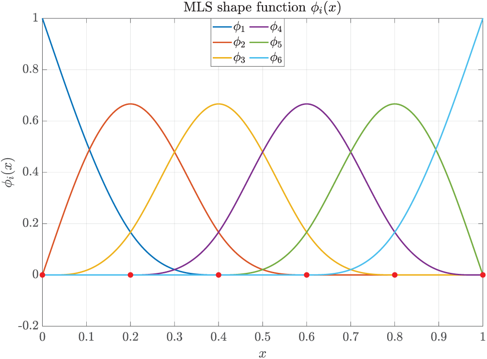
Figure 1: Schematic diagram of the MLS shape functions
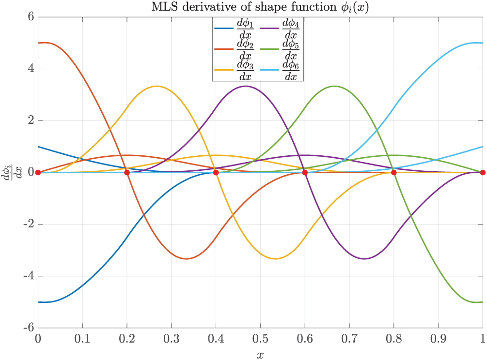
Figure 2: Schematic diagram of the MLS derivative of shape functions
This shape function can achieve high computational accuracy due to its foundation in least squares mathematical theory. However, the inversion of matrix
To simplify the high-computational cost are primarily focus of matrix
Applying Gram-Schmidt orthogonalization to the basis function
where
and
Therefore, the matrix
The resulting IMLS approximation shape function is therefore given by:
where
Evidently, the inverse of the modified matrix
2.3 The Interpolating MLS Approximation
Both the MLS and IMLS approximations lack interpolation properties, the penalty method is often used to impose the essential boundary condition in the corresponding meshless methods, which inevitably affects computational efficiency. To address this limitation, Ren et al. [63] proposed the interpolating MLS approximation based on the singular weight function.
When the zeroth-order basis function q = 1 is selected in the MLS method, thus the approximation function is
where
In the interpolating MLS approximation, the singular weight function can be selected as
or
and
Because
by orthogonalizing
The resulting interpolating MLS approximation shape function is therefore given by:
where
Therefore, the approximation function yields the following expression:
where
The interpolating MLS approximation satisfies the Kronecker delta property, endowing its shape functions with interpolation characteristics that permit direct imposition of essential boundary conditions. Moreover, the unknown coefficient vector
2.4 The Interpolating MLS Approximation with Nonsingular Weight Function
A drawback of the interpolating MLS approximation proposed by Ren et al. [63] is weight function singularity in constructing shape function, leading to the inevitable truncation errors. To overcome this limitation, Wang et al. studied a new interpolating MLS approximation [78] by replacing the singular weight function with the nonsingular alternative.
Inspired from Eq. (34), we can derive a new set of basis function such that the approximation function satisfies the interpolation property. Let
where
and
Therefore, the form of
where
From Eq. (42), we derive the same transformation for
the corresponding local approximation function is
From Eqs. (42) and (44), we have
Thus Eq. (48) can be simplified as
where
From Eqs. (47), (48) and (50), we have
Thus the resulting shape function is therefore given by:
where
In contrast to the interpolating MLS approximation developed by Ren et al. [63], the shape function formulation proposed by Wang et al. [78] allows arbitrary weight function selection from standard MLS approximation. This method not only eliminates computational challenges caused by weight functions singularities but also avoids the associated truncation errors.
The MLS, IMLS, and two type of interpolating MLS approximations are formulated for scalar function approximation. Bai et al. [102] developed the ICVMLS approximation to handle vector-valued function approximation.
For any function
and
In general, the simple linear basis function is adopted for the ICVMLS approximation, which can be written as
Define the following functional
where
Let
we get
where
Thus the approximation function can be obtained as
where the shape function is
Then Eq. (74) can be discretized as
and
If
Since the ICVMLS method yields the approximation function, the expression in Eq. (77) tends to zero. This demonstrates that only the real component of shape function needs to be retained to approximate the real-valued functions.
The use of the ICVMLS approximation with linear basis function for 2D shape function result in only 2 undetermined coefficients, as opposed to the 3 required by the MLS approximation, thereby directly lowering the matrix order in the computation.
3 The Improved EFG Methods for Partial Differential Equations and Nonlinear Mechanics Problems
3.1 The IEFG Method for 3D Steady Heat Conduction Problem in Anisotropic Media
This section employs a steady heat conduction problem to validate both the effectiveness and computational efficiency of the IEFG method.
The governing equation is
the Dirichlet and Neumann boundary conditions are
where
The functional corresponding to the governing heat conduction equation is constructed as follows:
where
The corresponding Galerkin weak form can be derived as
where
Assume that
Thus
where
By introducing the shape function, we obtain
The final equation can be derived
where
To verify the accuracy of the derived numerical solution formulation, we present the following numerical example, the governing equation is
the boundary conditions are
The exact solution [148] is
In order to calculate the accuracy of IEFG method, the relative error of the numerical solution is computed using the following formula:
In this example, the scaling parameter dmax is set to 1.3 and the penalty factor α is adjusted to 1.4 × 10³ in both EFG and IEFG methods. Fig. 3a shows the error variation of the EFG and IEFG methods for solving the heat conduction problem with different nodes in the problem domain. As shown in Fig. 3b, which presents the convergence rate of the IEFG method. It can be observed that the relative error decreases and tends to stabilize as the nodes increases, indicating that the IEFG method is convergent.
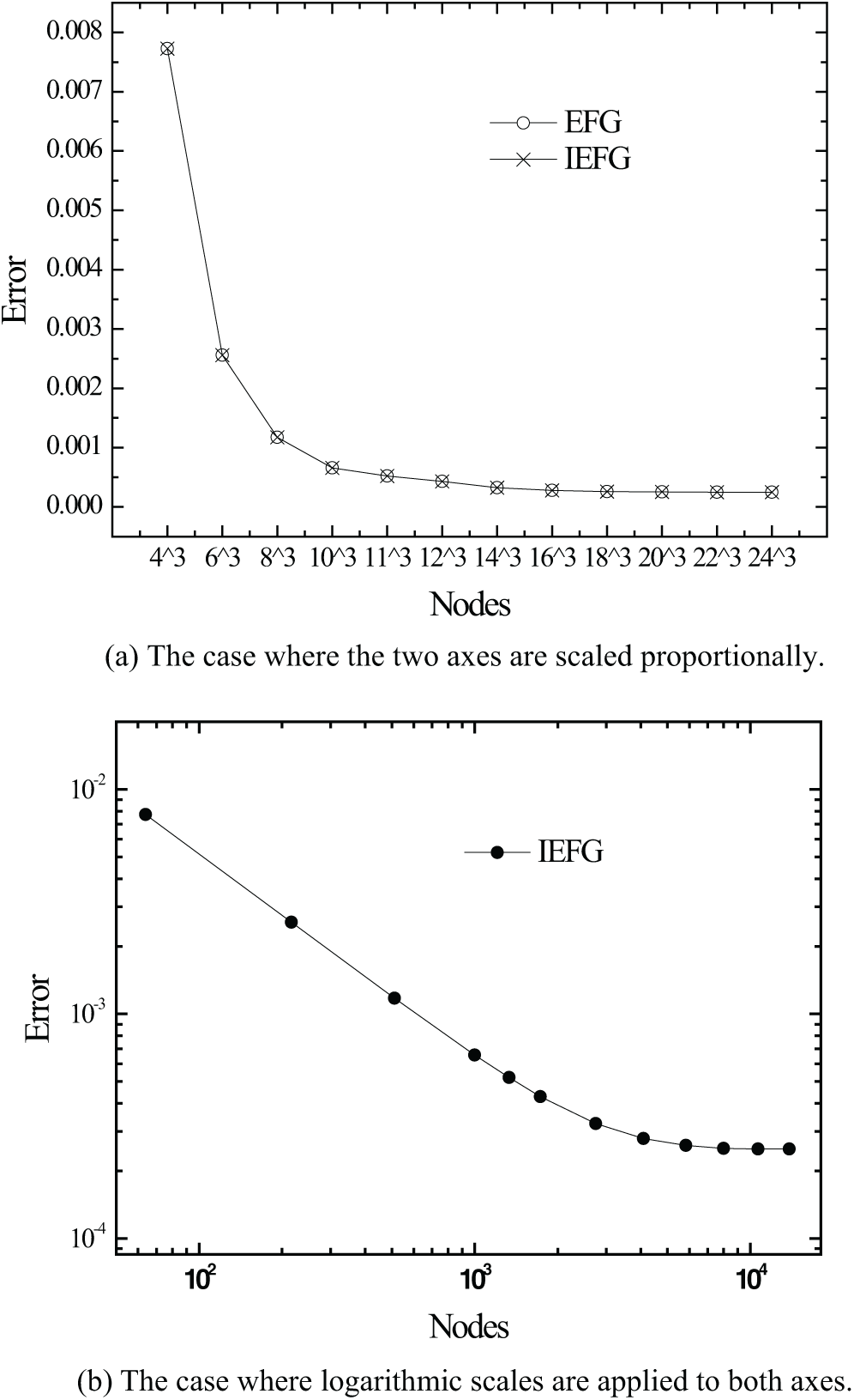
Figure 3: The relative error for different number of nodes
The IEFG and EFG methods are implemented with a node distribution of 11 × 11 × 11 and a corresponding background integral grid is 10 × 10 × 10, dmax is set to 1.3, and penalty factor α is set to 1.4 × 10³. Table 1 presents the computational errors and CPU time of two methods under appropriate parameters. Figs. 4–6 compare the exact and numerical solutions. Although both methods achieve a close approximation to the exact one, the IEFG method can save computational time.
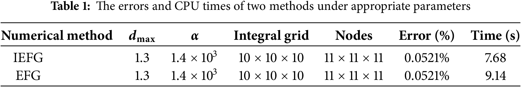
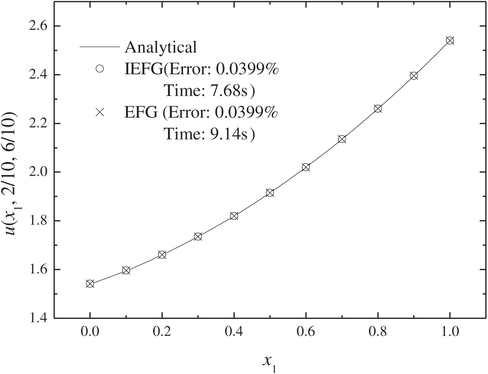
Figure 4: The temperature distribution along x1 direction
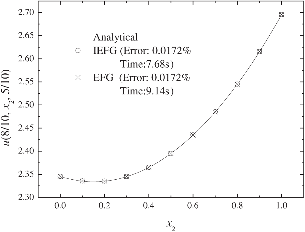
Figure 5: The temperature distribution along x2 direction
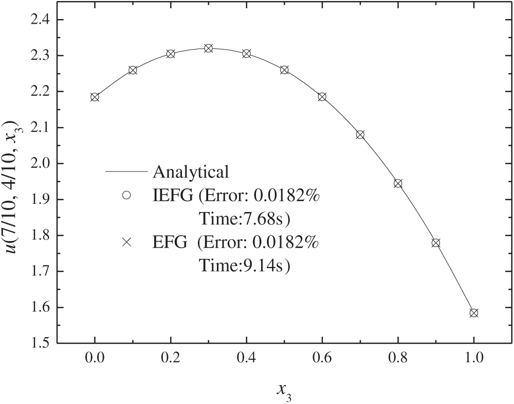
Figure 6: The temperature distribution along x3 direction
3.2 The IEFG Method for 3D Elastoplasticity Problem
In reference [149], Yu et al. selected the IEFG method to solve 3D elastoplasticity problems with four numerical examples. In this paper, we analyze an example with the hollow sphere subjected to uniform internal pressure.
Due to its symmetry, 1/8 of the structure is selected as the subject of the study. Fig. 7 illustrates 1/8 of the hollow sphere. The inner radius of the sphere is
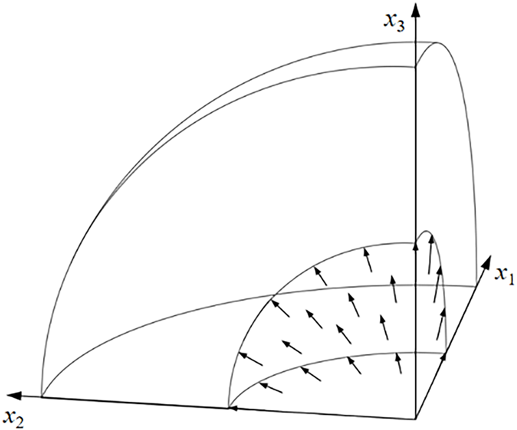
Figure 7: 1/8 hollow sphere under uniform internal pressure
We establish the nodal distribution for solving this problem using the IEFG method. The nodes on the coordinate plane are uniformly distributed along the circumferential direction and arranged evenly in the radial direction. 7 × 7 × 13 node distribution scheme is selected in Fig. 8.
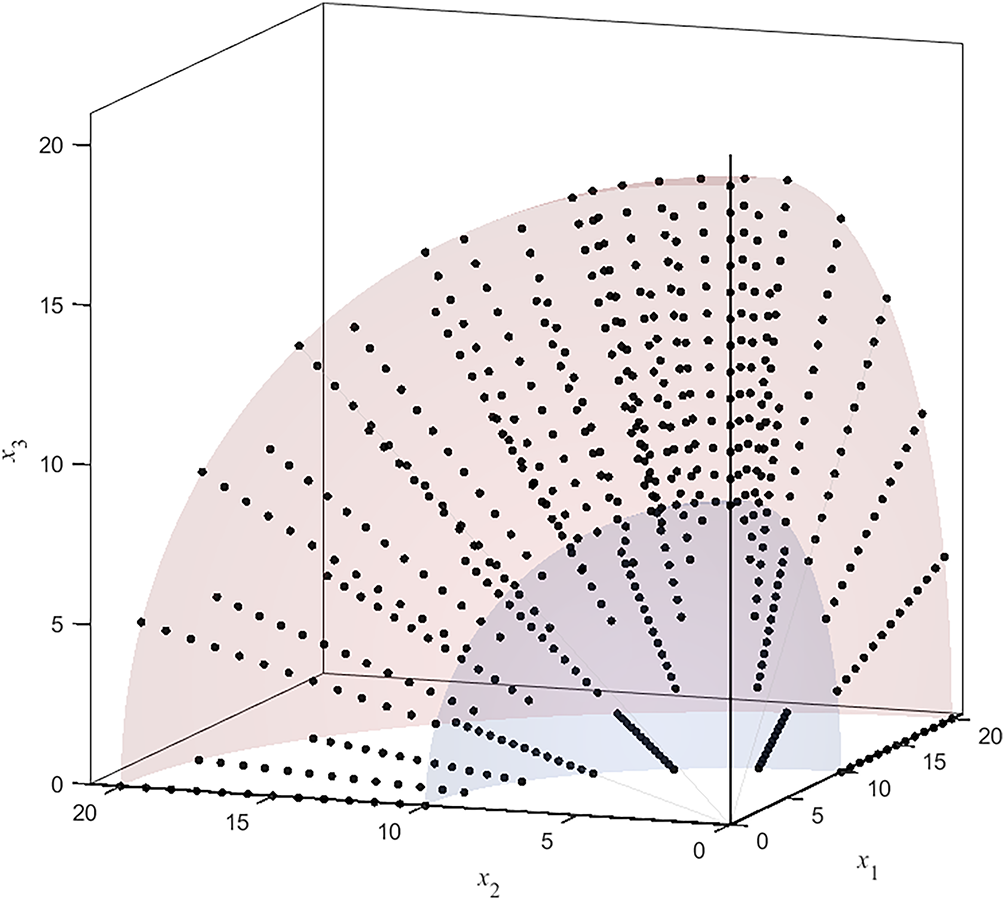
Figure 8: Node distribution in the problem domain
When the IEFG method is employed to solve this problem, the parameters are set as follows: dmax is 1.6, α is 1.0 × 10⁸, with the number of loading steps set to 50, and the weight function is a quintic spline function. The obtained error is 2.535%, and the CPU time is 759.4 s. When the EFG method is used to solve this problem, the parameters set are the same as those of the IEFG method, resulting in the same error. However, the computation time for the EFG method is 928.9 s.
Fig. 9 presents the numerical solutions of the IEFG method and the EFG method at x1 = 0 and x2 = 0. The figure indicates that both methods yield results consistent with the numerical solution obtained from ABAQUS.
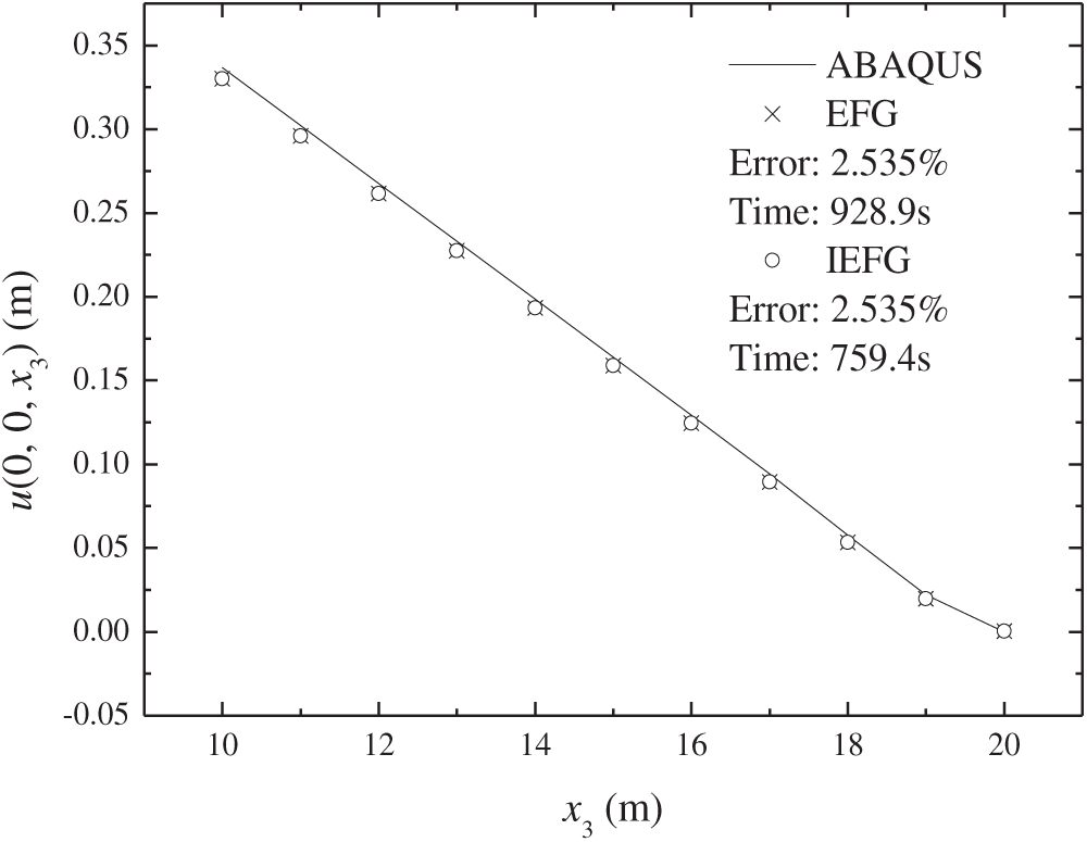
Figure 9: The numerical solution of displacement when x1 = 0 and x2 = 0
Fig. 10 shows 3D node displacement cloud plots of this example. It can be observed that the displacement gradually decreases along the radial direction.
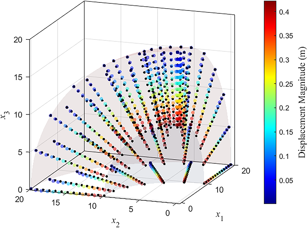
Figure 10: 3D node displacement cloud plot
3.3 The IEFG Method for 3D Large Deformation Problems
One of the fundamental advantages of meshless methods lies in their inherent capability to handle large deformation and crack propagation problems without mesh distortion that is unavoidable in FEM [150,151]. In this section, we implement the IEFG method for solving 3D elastic large deformation problems.
The equilibrium equation for large deformation problems at time
where
and
Following linearization of the equilibrium equations, we derive the corresponding weak integral form as:
where
By introducing the IMLS approximation, the displacement increment
and
Substituting Eqs. (112)–(115) into (111) yields:
where
Let
Eq. (117) can be simplified as
The above presents the IEFG method for elastic large deformation problems. For Eq. (146), the Newton-Raphson iteration method is employed in this work for numerical computation.
To verify the accuracy and efficiency of the derived numerical solution formulation, we consider a cantilever beam subjected to uniform load of
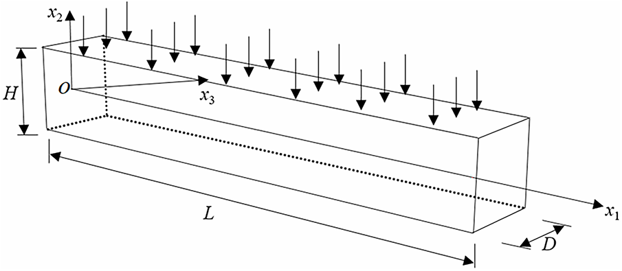
Figure 11: A cantilever beam subjected to a uniform load
The influence of node number on numerical accuracy should be considered. The total number of load steps is set to 20, with dmax = 3.5 and α = 1.2 × 10⁹, and the cubic spline function is selected. Fig. 12 presents the relative errors of numerical solutions under different node distributions. It can be seen that the number of nodes along
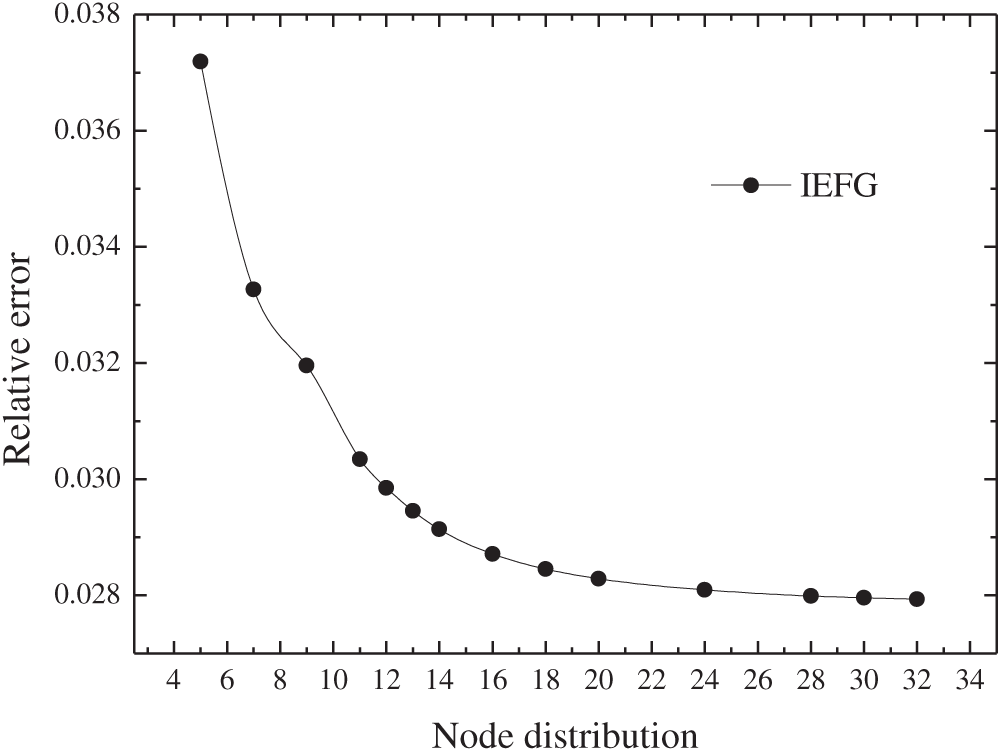
Figure 12: The error with different node distribution in x1 direction
The IEFG method for large deformation problems is employed for computation. As shown in Fig. 13, the computational domain is discretized with 13 × 5 × 5 nodes, 12 × 4 × 4 background integration cells, and the loading step is 20. Fig. 14 presents the numerical solutions of node displacements along the
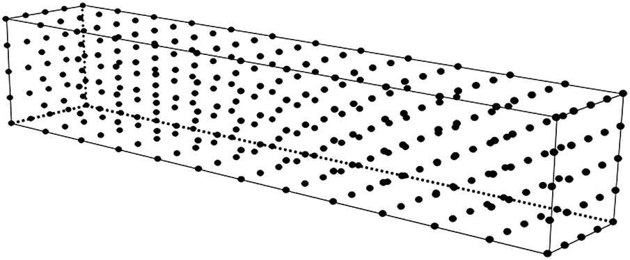
Figure 13: Nodes distribution in the beam
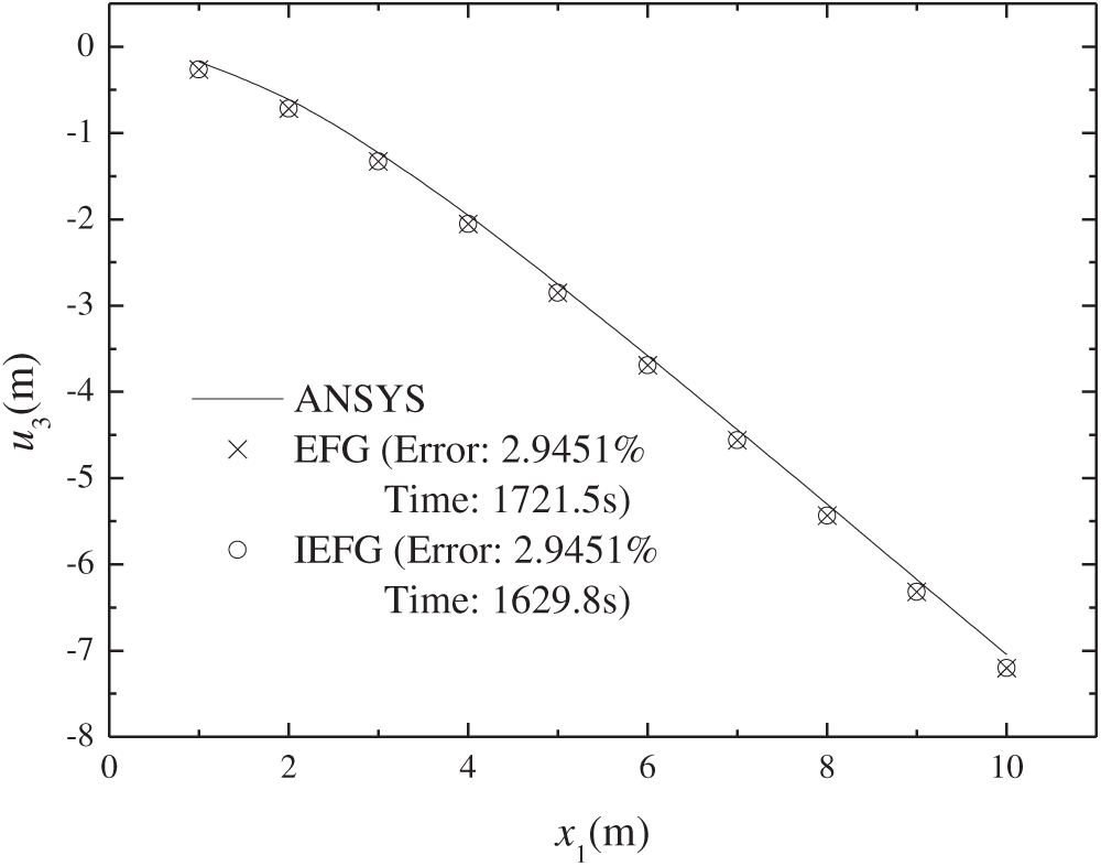
Figure 14: Numerical solutions of vertical displacements along x1 axis
The next example considers a square plate with a central hole subjected to uniformly distributed loads on both sides. Fig. 15 illustrates the plate with a central circular hole under tensile loads P on both sides. The plate has geometric dimensions of 10 m × 10 m × 1 m and a central hole radius of r = 1 m. The material parameters are as follows:
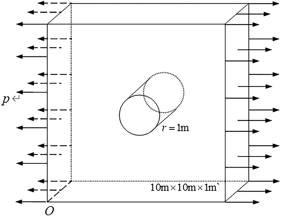
Figure 15: A centrally perforated plate under axial uniformly distributed load
Based on the symmetry of the model, 1/4 of the structure is considered for analysis. Fig. 16 illustrates the coordinate system and force distribution of the quarter-open plate, while Fig. 17 shows the nodal distribution scheme: points are arranged radially in a geometric progression with a common ratio of q, and uniformly along the circumferential direction. Node distribution of 11 × 11 × 2 is adopted in this numerical example.
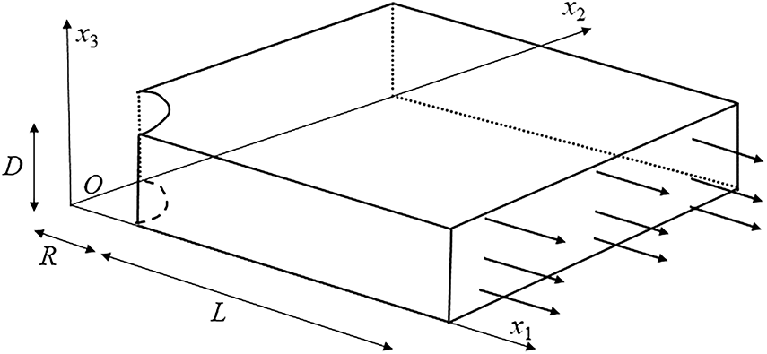
Figure 16: Force distribution diagram of a quarter-plate with a hole
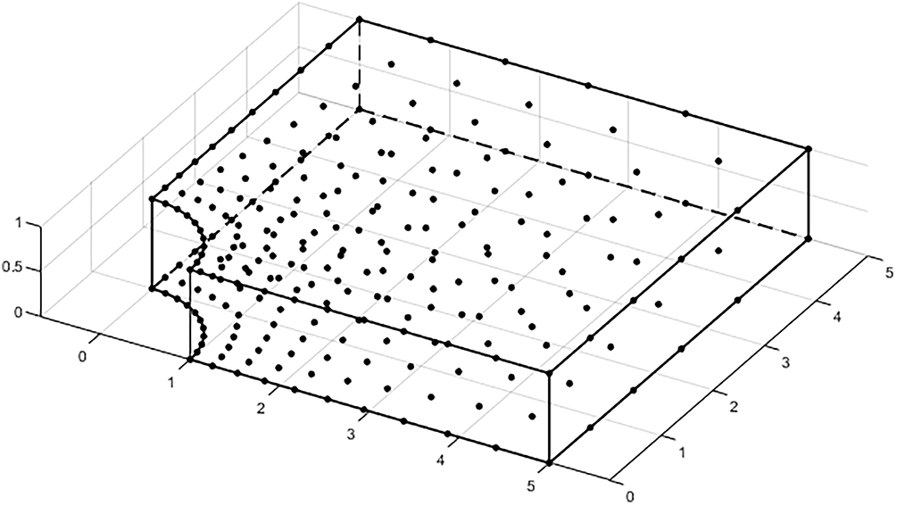
Figure 17: Node distribution
When the EFG method was employed to solve this problem, a cubic spline function was adopted as the weight function with the following parameter settings: dmax = 2.8, α = 1.0 × 10⁷, and the number of loading steps was 10. The resulting error was 0.9999%, and the computation time was 638.63 s. Under the same parameter settings, the IEFG method achieved the same error of 0.9999% while reducing the computation time to 563.62 s. Fig. 18 compares the results of the three numerical methods. It is shown that the IEFG method can save CPU time under similar computational accuracy.
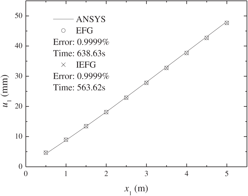
Figure 18: Comparison of results from different numerical methods
3.4 The DSIEFG Method and Dimension Coupling Method (DCM) for 3D Helmholtz Equations
As shown in Sections 3.1–3.3, the IEFG method can improve the computational speed of the EFG method, but the improvement remains relatively constrained for solving 3D problems.
To address the computational inefficiency of meshless methods in solving 3D complex mechanical problems, this section introduces the DSIEFG method and DCM for solving relatively simple 3D Helmholtz equations. A comparative analysis with the IEFG method is conducted to validate the superior computational efficiency of the proposed methods.
In this section, the 3D Helmholtz equation is given and the dimension splitting method (DSM) is introduced to decompose the 3D equation into multiple 2D forms. These 2D equations are discretized using the IEFG method, while the third direction is further discretized using the FDM [152] and FEM [137], respectively, yielding computational formulations for both approaches. A numerical example is then presented to validate the effectiveness and comparative advantages of each method.
3.4.1 The Weak Form of Helmholtz Equation Based on the DSM
The governing equation is
The boundary conditions are
Without loss of generality, we split the 3D problem into L + 1 layers along the x3 direction (See Fig. 19).
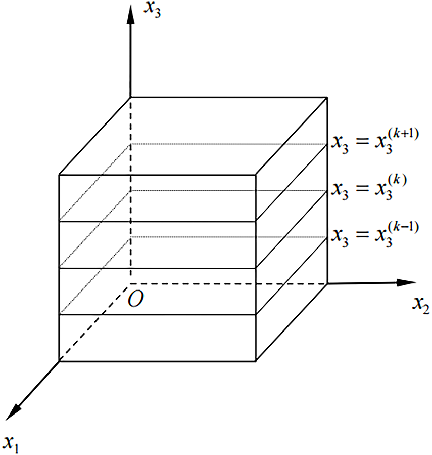
Figure 19: The problem domain is partitioned into L + 1 layers in x3-direction
The weak form obtained based on the DSM is
where
3.4.2 The IEFG Method for 2D Equations in Each Layer
By introducing 2D IMLS shape function, Eq. (150) is transformed as
where
thus the discretized equations are derived as
where
3.4.3 The FDM for 1D Equation in Splitting Direction
The FDM is introduced to discretize
If
where
If
Thus, finial equations are changed as
where
3.4.4 The FEM for 1D Equation in Splitting Direction
When the FEM is introduced to discretize
where
If the natural boundary conditions are known, thus the
and
3.4.5 An Example of Helmholtz Equation with Mix Boundary Conditions
The exact solution is
and
Table 2 shows the relative error and CPU time trends of the DSIEFG method with respect to mesh refinement in x1 direction. The results demonstrate an inverse relationship between error and computational cost: as the mesh density increases in the splitting direction, the relative error decreases from 1.3667% to 0.7729%, while the computation time increases from 73.8 to 263.9 s. Therefore, when selecting the natural boundary condition as the splitting direction, considering both computational accuracy and time, we chose a mesh number of 360, and a relatively small error of 0.8830% was achieved, with a corresponding CPU time of 160.3 s.

A comparison was conducted on the computational accuracy and time of the IEFG method, the DSIEFG method, and the DCM when solving this problem under different splitting directions, the parameter selections are shown in Table 3. The results indicate that when the x1-axis is chosen as the splitting direction, the DCM can directly and efficiently handle the natural boundary conditions along the dimensional splitting direction without requiring many layers, thereby significantly improving the computational efficiency compared to the DSIEFG method.
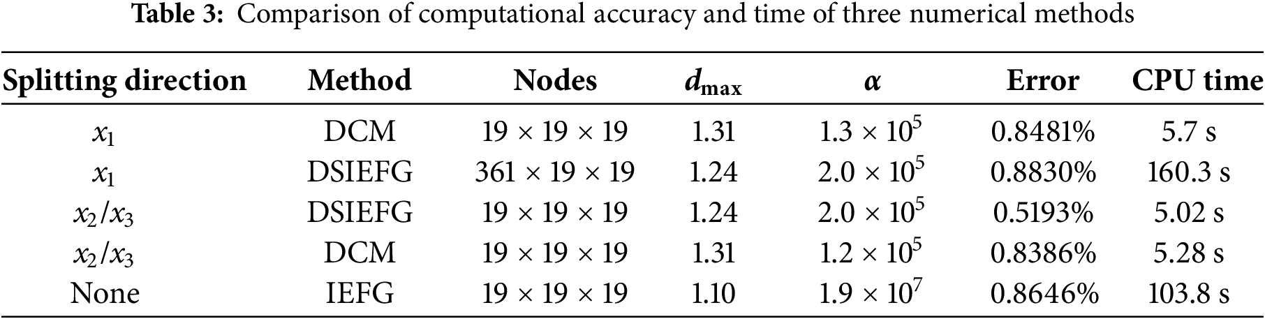
However, when the x2 or x3 axis is selected as the splitting direction, the parameter selections are shown in Table 3. Both the dimension splitting meshless methods significantly improve the computational speed of the IEFG method, and the DSIEFG method demonstrates superior computational accuracy and speed compared to the DCM. Owing to its theoretical simplicity relative to the FEM, the FDM is easier to apply to relatively simple partial differential equations (PDEs) possessing essential boundary conditions.
When the x1-axis is selected as the splitting direction, the numerical solutions of the three methods are compared with the analytical solution. As shown in Figs. 20–22, it can be observed that the numerical solutions of these three methods agree well with the analytical solution.
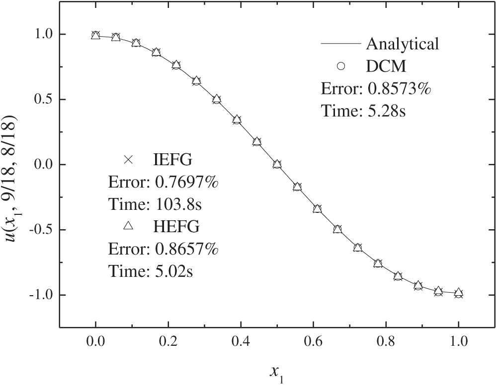
Figure 20: Numerical results of three methods in x1 direction
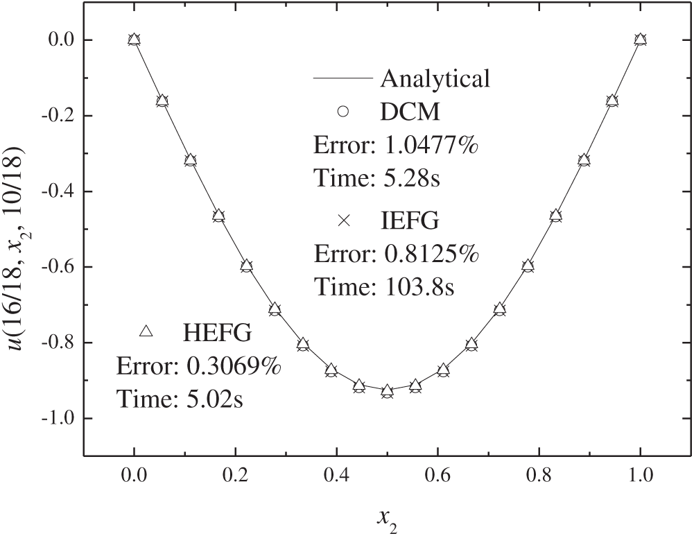
Figure 21: Numerical results of three methods in x2 direction
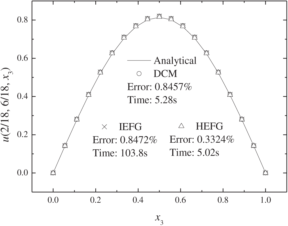
Figure 22: Numerical results of three methods in x3 direction
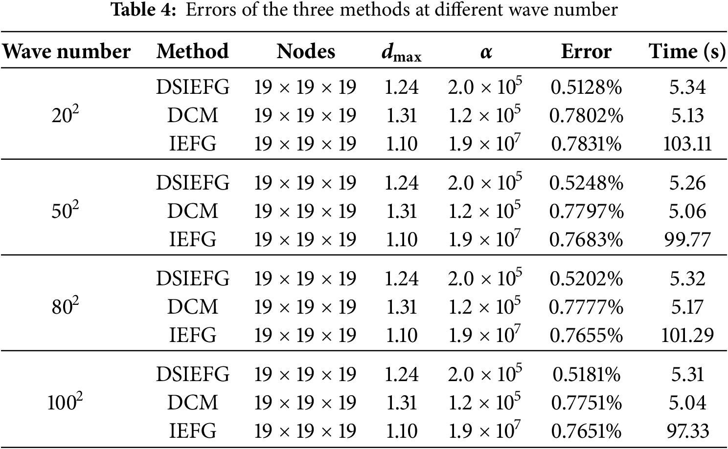
Table 4 shows the relative error with respect to the different wave numbers, demonstrating the stability of three numerical methods.
Despite the efficiency of two-dimensional splitting meshless methods in solving Helmholtz equations, their performance remains limited in handling complex 3D problems with intricate geometric domains. Therefore, the corresponding methods require further improvements to enhance their applicability.
4 Conclusions and Further Directions
This paper provides a comprehensive review of the EFG method and its various improved versions. As these improvements are primarily centered on the shape functions, we systematically summarize the derivations of their key formulations. To demonstrate the superiority of the improved methods, the IEFG method is applied to solve both 3D heat conduction, elastoplasticity and large deformation problems. Numerical examples verify its effectiveness and computational efficiency over the EFG method. Furthermore, the DSIEFG method and the DCM are introduced for solving 3D Helmholtz equations. Numerical experiment confirms that these methods significantly enhance computational performance compared to the IEFG in handling 3D problems, marking a substantial advancement in meshless computational mechanics.
While significant progress has been made in the improved EFG methods, several challenges remain in the research on the improved EFG methods, particularly in the following key areas requiring future investigation:
1) The dimension splitting meshless methods have primarily been applied to 3D partial differential equations and relatively simple 3D elasticity problems. However, some challenges persist when addressing anisotropic heat conduction problems with second-order mixed partial derivatives and more complex 3D mechanics analyses. Consequently, the theoretical framework of dimension splitting meshless methods requires further refinement to adequately address large-scale, complex 3D mechanical problems.
2) Although the ICVEFG method has been widely applied in 2D computational mechanics, existing applications in 3D analyses have primarily focused on solving partial differential equations and elastoplastic problems. Its extension to 3D complex mechanics applications remains an important and largely unexplored research area.
3) While the 2D interpolating ICVEFG method has been well established in the literature, its extension to 3D problems has not yet been investigated. The development of such 3D formulations presents a critical research frontier with significant potential applications.
4) The integration of the improved EFG methods with neural networks for solving inverse problems represents a promising and potentially transformative direction for future research in computational mechanics.
Acknowledgement: None.
Funding Statement: This work was supported by the National Natural Science Foundation of China (Grant No. 12271341).
Author Contributions: Study conception and design: Yumin Cheng, Heng Cheng; data collection: Yichen Yang; analysis and interpretation of results: Heng Cheng; draft manuscript preparation: Heng Cheng, Yichen Yang. All authors reviewed the results and approved the final version of the manuscript.
Availability of Data and Materials: The data can be obtained from the literature cited in this paper. More detailed data will be shared on reasonable request to the corresponding author.
Ethics Approval: Not applicable.
Conflicts of Interest: The authors declare no conflicts of interest to report regarding the present study.
References
1. Liu WK, Li S, Park HS. Eighty years of the finite element method: birth, evolution, and future. Arch Comput Meth Eng. 2022;29(6):4431–53. doi:10.1007/s11831-022-09740-9. [Google Scholar] [CrossRef]
2. Lucy LB. A numerical approach to the testing of the fission hypothesis. Astron J. 1977;82:1013. doi:10.1086/112164. [Google Scholar] [CrossRef]
3. Lancaster P, Salkauskas K. Surfaces generated by moving least squares methods. Math Comp. 1981;37(155):141–58. doi:10.1090/s0025-5718-1981-0616367-1. [Google Scholar] [PubMed] [CrossRef]
4. Nayroles B, Touzot G, Villon P. Generalizing the finite element method: diffuse approximation and diffuse elements. Comput Mech. 1992;10(5):307–18. doi:10.1007/BF00364252. [Google Scholar] [CrossRef]
5. Belytschko T, Lu YY, Gu L. Element-free Galerkin methods. Int J Numer Methods Eng. 1994;37(2):229–56. doi:10.1002/nme.1620370205. [Google Scholar] [CrossRef]
6. Liu WK, Jun S, Zhang YF. Reproducing kernel particle methods. Numerical Methods Fluids. 1995;20(8–9):1081–106. doi:10.1002/fld.1650200824. [Google Scholar] [CrossRef]
7. Oñate E, Idelsohn S, Zienkiewicz OC, Taylor RL. A finite point method in computational mechanics. applications to convective transport and fluid flow. Int J Numer Meth Eng. 1996;39(22):3839–66. doi:10.1002/(SICI)1097-0207(19961130)39:223839::AID-NME27>3.0.CO;2-R. [Google Scholar] [CrossRef]
8. Babuška I, Melenk JM. The partition of unity method. Int J Numer Methods Eng. 1997;40(4):727–58. doi: 10.1002/(sici)1097-0207(19970228)40:4<727::aid-nme86>3.3.co;2-e. [Google Scholar] [CrossRef]
9. Pollandt R. Solving nonlinear differential equations of mechanics with the boundary element method and radial basis functions. Int J Numer Meth Eng. 1997;40(1):61–73. doi:10.1002/(SICI)1097-0207(19970115)40:. [Google Scholar] [CrossRef]
10. Mukherjee YX, Mukherjee S. The boundary node method for potential problems. Int J Numer Methods Eng. 1997;40(5):797–815. doi: 10.1002/(sici)1097-0207(19970315)40:5<797::aid-nme89>3.3.co;2-r. [Google Scholar] [CrossRef]
11. Sukumar N, Moran B, Belytschko T. The natural element method in solid mechanics. Int J Numer Meth Engng. 1998;43(5):839–87. doi:10.1002/(sici)1097-0207(19981115)43:5<839::aid-nme423>3.0.co;2-r. [Google Scholar] [CrossRef]
12. Atluri SN, Zhu T. A new Meshless Local Petrov-Galerkin (MLPG) approach in computational mechanics. Comput Mech. 1998;22(2):117–27. doi:10.1007/s004660050346. [Google Scholar] [CrossRef]
13. Atluri SN, Sladek J, Sladek V, Zhu T. The local boundary integral equation (LBIE) and it’s meshless implementation for linear elasticity. Comput Mech. 2000;25(2):180–98. doi:10.1007/s004660050468. [Google Scholar] [CrossRef]
14. Liu GR, Gu YT. A point interpolation method for two-dimensional solids. Int J Numer Methods Eng. 2001;50(4):937–51. doi:10.1002/1097-0207(20010210)50:. [Google Scholar] [CrossRef]
15. Zhang X, Liu XH, Song KZ, Lu MW. Least-squares collocation meshless method. Numerical Meth Eng. 2001;51(9):1089–100. doi:10.1002/nme.200. [Google Scholar] [CrossRef]
16. Zhang JM, Yao ZH, Li H. A hybrid boundary node method. Int J Numer Methods Eng. 2002;53(4):751–63. doi:10.1002/nme.313. [Google Scholar] [CrossRef]
17. Gu L. Moving Kriging interpolation and element-free Galerkin method. Int J Numer Methods Eng. 2003;56(1):1–11. doi:10.1002/nme.553. [Google Scholar] [CrossRef]
18. Idelsohn SR, Oñate E, Calvo N, Del Pin F. The meshless finite element method. Int J Numer Methods Eng. 2003;58(6):893–912. doi:10.1002/nme.798. [Google Scholar] [CrossRef]
19. Li X. Error estimates for the moving least-square approximation and the element-free Galerkin method in n-dimensional spaces. Appl Numer Math. 2016;99:77–97. doi:10.1016/j.apnum.2015.07.006. [Google Scholar] [CrossRef]
20. Zhang J, Zhou G, Gong S, Wang S. Transient heat transfer analysis of anisotropic material by using Element-Free Galerkin method. Int Commun Heat Mass Transf. 2017;84(1):134–43. doi:10.1016/j.icheatmasstransfer.2017.04.003. [Google Scholar] [CrossRef]
21. Qin X, Duan X, Hu G, Su L, Wang X. An Element-free Galerkin method for solving the two-dimensional hyperbolic problem. Appl Math Comput. 2018;321(1):106–20. doi:10.1016/j.amc.2017.10.040. [Google Scholar] [CrossRef]
22. Wang HS. An extended element-free Galerkin method for thermo-mechanical dynamic fracture in linear and nonlinear materials. Comput Mater Sci. 2015;98(1):366–71. doi:10.1016/j.commatsci.2014.10.050. [Google Scholar] [CrossRef]
23. Shao Y, Duan Q, Qiu S. Adaptive consistent element-free Galerkin method for phase-field model of brittle fracture. Comput Mech. 2019;64(3):741–67. doi:10.1007/s00466-019-01679-2. [Google Scholar] [CrossRef]
24. Lin Q, Wang J, Hong J, Liu Z, Wang Z. A biomimetic generative optimization design for conductive heat transfer based on element-free Galerkin method. Int Commun Heat Mass Transf. 2019;100(17):67–72. doi:10.1016/j.icheatmasstransfer.2018.12.001. [Google Scholar] [CrossRef]
25. Meng JN, Pan G, Cao YH. Element-Free Galerkin method for dynamic boundary flow problems. Mod Phys Lett B. 2020;34(24):2050257. doi:10.1142/s0217984920502577. [Google Scholar] [CrossRef]
26. Zhou L, Yang H, Ma L, Zhang S, Li X, Ren S, et al. On the static analysis of inhomogeneous magneto-electro-elastic plates in thermal environment via element-free Galerkin method. Eng Anal Bound Elem. 2022;134(1):539–52. doi:10.1016/j.enganabound.2021.11.002. [Google Scholar] [CrossRef]
27. Cai LQ, Wang XD, Yao M. Non-uniform shrinkage analysis of round billet using element-free Galerkin method. J Iron Steel Res Int. 2022;29(1):80–7. doi:10.1007/s42243-021-00638-7. [Google Scholar] [CrossRef]
28. Yan X. Free vibration analysis of a rotating nanobeam using integral form of Eringen’s nonlocal theory and element-free Galerkin method. Appl Phys A. 2022;128(8):641. doi:10.1007/s00339-022-05714-7. [Google Scholar] [CrossRef]
29. Li Y, Liu C, Li W, Chai Y. Numerical investigation of the element-free Galerkin method (EFGM) with appropriate temporal discretization techniques for transient wave propagation problems. Appl Math Comput. 2023;442:127755. doi:10.1016/j.amc.2022.127755. [Google Scholar] [CrossRef]
30. Shen Q, Ding R, Yao Y. The element-free Galerkin method for the variational-hemivariational inequality of the dynamic Signorini-Tresca contact problems with friction in elastic materials. Commun Nonlinear Sci Numer Simul. 2023;116(3–4):106816. doi:10.1016/j.cnsns.2022.106816. [Google Scholar] [CrossRef]
31. Zheng J, Yang X, Long S. Topology optimization with geometrically non-linear based on the element free Galerkin method. Int J Mech Mater Des. 2015;11(3):231–41. doi:10.1007/s10999-014-9257-y. [Google Scholar] [CrossRef]
32. Wang S, Yi W, Qian H, Ju L. Multi-objective topology optimization of thermoelastic structures based on points density using element-free Galerkin method. Eng Struct. 2025;326(10):119515. doi:10.1016/j.engstruct.2024.119515. [Google Scholar] [CrossRef]
33. Zhang J, Zhang Z, Wu S, Zhao L, Wu S, Zuo Z, et al. Topology optimization of multi-material structures with length-scale control based on Neural Style Transfer and element-free Galerkin method. Eur J Mech A. 2025;112:105645. doi:10.1016/j.euromechsol.2025.105645. [Google Scholar] [CrossRef]
34. Chen W, Luo WM, Chen SY, Peng LX. A FSDT meshfree method for free vibration analysis of arbitrary laminated composite shells and spatial structures. Compos Struct. 2022;279(5):114763. doi:10.1016/j.compstruct.2021.114763. [Google Scholar] [CrossRef]
35. Qin X, Xiang J, He X, Shen Y, Chen W, Peng LX. Buckling analysis of skew and circular stiffened plates using the Galerkin meshless method. Acta Mech. 2022;233(5):1789–817. doi:10.1007/s00707-022-03191-w. [Google Scholar] [CrossRef]
36. Ma H, Chen J, Deng J. Error analysis of the element-free Galerkin method for a nonlinear plate problem. Comput Math Appl. 2024;163(1):56–65. doi:10.1016/j.camwa.2024.03.020. [Google Scholar] [CrossRef]
37. Peng L, Zhang Z, Wei D, Tang P, Mo G. Nonlinear analysis of corrugated core sandwich plates using the element-free Galerkin method. Buildings. 2025;15(8):1235. doi:10.3390/buildings15081235. [Google Scholar] [CrossRef]
38. Yuan B, Fang W, Li J, Cai Y, Qu Z, Wang Z. A coupled finite element-element-free Galerkin method for simulating viscous pressure forming. Eng Anal Bound Elem. 2016;68(6):86–102. doi:10.1016/j.enganabound.2016.04.003. [Google Scholar] [CrossRef]
39. Zhang Y, Ge W, Zhang Y, Zhao Z. Topology optimization method with direct coupled finite element-element-free Galerkin method. Adv Eng Softw. 2018;115(2):217–29. doi:10.1016/j.advengsoft.2017.09.012. [Google Scholar] [CrossRef]
40. Zhang X, Xiang S. An efficient variational multiscale element free Galerkin method based on adaptive TR-AB2 scheme for convection-diffusion equations. Eng Anal Bound Elem. 2024;158(2):211–23. doi:10.1016/j.enganabound.2023.10.026. [Google Scholar] [CrossRef]
41. Fan Y, Zhang X. The reduced variational multiscale element free Galerkin method for three-dimensional steady incompressible Stokes and Navier-Stokes equations. Eng Anal Bound Elem. 2024;169(1):105984. doi:10.1016/j.enganabound.2024.105984. [Google Scholar] [CrossRef]
42. Ghorbani M, Noormohammadi N, Boroomand B. Enrichment of the element free Galerkin method for cracks and notches without a priori knowledge of the analytical singularity order. Comput Math Appl. 2024;162:155–79. doi:10.1016/j.camwa.2024.03.007. [Google Scholar] [CrossRef]
43. Cheng YM, Chen MJ. A boundary element-free method for linear elasticity. Acta Mech Sin. 2003;35(2):181–6. (In Chinese). [Google Scholar]
44. Zhang Z, Zhao P, Liew KM. Improved element-free Galerkin method for two-dimensional potential problems. Eng Anal Bound Elem. 2009;33(4):547–54. doi:10.1016/j.enganabound.2008.08.004. [Google Scholar] [CrossRef]
45. Zhang Z, Zhao P, Liew KM. Analyzing three-dimensional potential problems with the improved element-free Galerkin method. Comput Mech. 2009;44(2):273–84. doi:10.1007/s00466-009-0364-9. [Google Scholar] [CrossRef]
46. Zhang Z, Wang J, Cheng Y, Liew KM. The improved element-free Galerkin method for three-dimensional transient heat conduction problems. Sci China Phys Mech Astron. 2013;56(8):1568–80. doi:10.1007/s11433-013-5135-0. [Google Scholar] [CrossRef]
47. Cheng RJ, Liew KM. Analyzing modified equal width (MEW) wave equation using the improved element-free Galerkin method. Eng Anal Bound Elem. 2012;36(9):1322–30. doi:10.1016/j.enganabound.2012.03.013. [Google Scholar] [CrossRef]
48. Cheng RJ, Wei Q. Analysis of the generalized Camassa and Holm equation with the improved element-free Galerkin method. Chin Phys B. 2013;22(6):154–9. (In Chinese). doi:10.1088/1674-1056/22/6/060209. [Google Scholar] [CrossRef]
49. Peng MJ, Li RX, Cheng YM. Analyzing three-dimensional viscoelasticity problems via the improved element-free Galerkin (IEFG) method. Eng Anal Bound Elem. 2014;40(3):104–13. doi:10.1016/j.enganabound.2013.11.018. [Google Scholar] [CrossRef]
50. Zheng G, Cheng Y. The improved element-free Galerkin method for diffusional drug release problems. Int J Appl Mechanics. 2020;12(8):2050096. doi:10.1142/s1758825120500969. [Google Scholar] [CrossRef]
51. Yan J, Cheng Y. Deep learning-meshless method for inverse potential problems. Int J Appl Mechanics. 2024;16(8):2450069. doi:10.1142/s1758825124500698. [Google Scholar] [CrossRef]
52. Zhang LW, Deng YJ, Liew KM. An improved element-free Galerkin method for numerical modeling of the biological population problems. Eng Anal Bound Elem. 2014;40:181–8. doi:10.1016/j.enganabound.2013.12.008. [Google Scholar] [CrossRef]
53. Li X, Chen H, Wang Y. Error analysis in Sobolev spaces for the improved moving least-square approximation and the improved element-free Galerkin method. Appl Math Comput. 2015;262:56–78. doi:10.1016/j.amc.2015.04.002. [Google Scholar] [CrossRef]
54. Tang YZ, Li XL. Meshless analysis of an improved element-free Galerkin method for linear and nonlinear elliptic problems. Chin Phys B. 2017;26(3):219–29. (In Chinese). doi:10.1088/1674-1056/26/3/030203. [Google Scholar] [CrossRef]
55. Li X, Li S. Analyzing the nonlinear p-Laplacian problem with the improved element-free Galerkin method. Eng Anal Bound Elem. 2019;100:48–58. doi:10.1016/j.enganabound.2018.04.004. [Google Scholar] [CrossRef]
56. Tan Y, Li XL. A meshless algorithm with the improved moving least square approximation for nonlinear improved Boussinesq equation. Chin Phys B. 2021;30(1):153–60. (In Chinese). doi:10.1088/1674-1056/abaed7. [Google Scholar] [CrossRef]
57. Debbabi I, BelhadjSalah H. Analysis of thermo-elastic problems using the improved element-free Galerkin method. Comput Appl Math. 2018;37(2):1379–94. doi:10.1007/s40314-016-0401-1. [Google Scholar] [CrossRef]
58. Mousavi H, Azhari M, Saadatpour MM, Sarrami-Foroushani S. A coupled improved element free Galerkin-finite strip (IEFG-FS) method for free vibration analysis of plate. Int J Appl Mechanics. 2019;11(10):1950103. doi:10.1142/s1758825119501035. [Google Scholar] [CrossRef]
59. Guo H, Cao S, Yang T, Chen Y. Vibration of laminated composite quadrilateral plates reinforced with graphene nanoplatelets using the element-free IMLS-Ritz method. Int J Mech Sci. 2018;142–143(2):610–21. doi:10.1016/j.ijmecsci.2018.05.029. [Google Scholar] [CrossRef]
60. Guo H, Cao S, Yang T, Chen Y. Geometrically nonlinear analysis of laminated composite quadrilateral plates reinforced with graphene nanoplatelets using the element-free IMLS-Ritz method. Compos Part B Eng. 2018;154(1):216–24. doi:10.1016/j.compositesb.2018.08.018. [Google Scholar] [CrossRef]
61. Huang K, Guo H, Qin Z, Cao S, Chen Y. Flutter analysis of laminated composite quadrilateral plates reinforced with graphene nanoplatelets using the element-free IMLS-Ritz method. Aerosp Sci Technol. 2020;103(3):105915. doi:10.1016/j.ast.2020.105915. [Google Scholar] [CrossRef]
62. Guo H, Huang K, Lei Z. Dynamic analysis of rotating laminated composite cantilever plates reinforced with graphene nanoplatelets using the element-free IMLS-Ritz method. Mech Based Des Struct Mach. 2022;50(10):3352–69. doi:10.1080/15397734.2020.1803083. [Google Scholar] [CrossRef]
63. Ren HP, Cheng YM, Zhang W. An improved boundary element-free method (IBEFM) for two-dimensional potential problems. Chin Phys B. 2009;18(10):4065–73. (In Chinese). [Google Scholar]
64. Wang J, Sun F. An interpolating meshless method for the numerical simulation of the time-fractional diffusion equations with error estimates. Eng Comput. 2019;37(2):730–52. doi:10.1108/ec-03-2019-0117. [Google Scholar] [CrossRef]
65. Li X, Wang Q. Analysis of the inherent instability of the interpolating moving least squares method when using improper polynomial bases. Eng Anal Bound Elem. 2016;73(10):21–34. doi:10.1016/j.enganabound.2016.08.012. [Google Scholar] [CrossRef]
66. Ren HP, Cheng YM. The interpolating element-free Galerkin (IEFG) method for two-dimensional elasticity problems. Int J Appl Mech. 2011;3(4):735–58. doi:10.1142/s1758825111001214. [Google Scholar] [CrossRef]
67. Ren HP, Wang LP, Zhao N. An interpolating element-free Galerkin (IEFG) method for steady-state heat conduction problems. Int J Appl Mech. 2014;6(3):1450024. doi:10.1142/s1758825114500240. [Google Scholar] [CrossRef]
68. Zhang G, Zhang F, Ren H. Accuracy analysis of interpolating element-free Galerkin (IEFG) method in solving transient heat conduction problems. Int J Appl Mechanics. 2016;8(6):1650078. doi:10.1142/s1758825116500782. [Google Scholar] [CrossRef]
69. Liu D, Cheng YM. The interpolating element-free Galerkin (IEFG) method for three-dimensional potential problems. Eng Anal Bound Elem. 2019;108(1–4):115–23. doi:10.1016/j.enganabound.2019.08.021. [Google Scholar] [CrossRef]
70. Wu Q, Peng P, Cheng Y. The interpolating element-free Galerkin method for elastic large deformation problems. Sci China Technol Sci. 2021;64(2):364–74. doi:10.1007/s11431-019-1583-y. [Google Scholar] [CrossRef]
71. Sun F, Wang J. Interpolating element-free Galerkin method for the regularized long wave equation and its error analysis. Appl Math Comput. 2017;315(2):54–69. doi:10.1016/j.amc.2017.07.052. [Google Scholar] [CrossRef]
72. Zhang PX, Peng MJ. Interpolating element-free Galerkin method for viscoelasticity problems. Acta Phys Sin. 2019;68(17):41–52. (In Chinese). [Google Scholar]
73. Dehghan M, Abbaszadeh M. Error analysis and numerical simulation of magnetohydrodynamics (MHD) equation based on the interpolating element free Galerkin (IEFG) method. Appl Numer Math. 2019;137(1):252–73. doi:10.1016/j.apnum.2018.10.004. [Google Scholar] [CrossRef]
74. Shen Q, Ding R, Zhu Z. Convergence analysis and error estimates of the interpolating element-free Galerkin method for the evolutionary variational inequality of the second-order in time. Comput Appl Math. 2020;39(2):130. doi:10.1007/s40314-020-01154-2. [Google Scholar] [CrossRef]
75. Ding R, Ding C, Shen Q. The interpolating element-free Galerkin method for the p-Laplace double obstacle mixed complementarity problem. J Glob Optim. 2023;86(3):781–820. doi:10.1007/s10898-022-01260-x. [Google Scholar] [CrossRef]
76. Zhang T, Li X. A variational multiscale interpolating element-free Galerkin method for convection-diffusion and Stokes problems. Eng Anal Bound Elem. 2017;82:185–93. doi:10.1016/j.enganabound.2017.06.013. [Google Scholar] [CrossRef]
77. Zhang T, Li X. Variational multiscale interpolating element-free Galerkin method for the nonlinear Darcy-Forchheimer model. Comput Math Appl. 2020;79(2):363–77. doi:10.1016/j.camwa.2019.07.003. [Google Scholar] [CrossRef]
78. Wang JF, Sun FX, Cheng YM. An improved interpolating element-free Galerkin method with a nonsingular weight function for two-dimensional potential problems. Chin Phys B. 2012;21(9):53–9. (In Chinese). doi:10.1088/1674-1056/21/9/090204. [Google Scholar] [CrossRef]
79. Sun FX, Wang JF, Cheng YM. An improved interpolating element-free Galerkin method for elasticity. Chin Phys B. 2013;22(12):120203. doi:10.1088/1674-1056/22/12/120203. [Google Scholar] [CrossRef]
80. Sun F, Wang J, Cheng Y. An improved interpolating element-free Galerkin method for elastoplasticity via nonsingular weight functions. Int J Appl Mechanics. 2016;8(8):1650096. doi:10.1142/s1758825116500964. [Google Scholar] [CrossRef]
81. Dehghan M, Abbaszadeh M, Mohebbi A. Analysis of two methods based on Galerkin weak form for fractional diffusion-wave: meshless interpolating element free Galerkin (IEFG) and finite element methods. Eng Anal Bound Elem. 2016;64(5):205–21. doi:10.1016/j.enganabound.2015.11.011. [Google Scholar] [CrossRef]
82. Abbaszadeh M, Dehghan M. Numerical and analytical investigations for solving the inverse tempered fractional diffusion equation via interpolating element-free Galerkin (IEFG) method. J Therm Anal Calorim. 2021;143(3):1917–33. doi:10.1007/s10973-020-10116-z. [Google Scholar] [CrossRef]
83. Abbaszadeh M, Dehghan M. Investigation of the Oldroyd model as a generalized incompressible Navier-Stokes equation via the interpolating stabilized element free Galerkin technique. Appl Numer Math. 2020;150(4):274–94. doi:10.1016/j.apnum.2019.08.025. [Google Scholar] [CrossRef]
84. Abbaszadeh M, Dehghan M, Navon IM. A proper orthogonal decomposition variational multiscale meshless interpolating element-free Galerkin method for incompressible magnetohydrodynamics flow. Int J Numer Meth Fluids. 2020;92(10):1415–36. doi:10.1002/fld.4834. [Google Scholar] [CrossRef]
85. Liu F, Cheng Y. The improved element-free Galerkin method based on the nonsingular weight functions for inhomogeneous swelling of polymer gels. Int J Appl Mechanics. 2018;10(4):1850047. doi:10.1142/s1758825118500473. [Google Scholar] [CrossRef]
86. Liu F, Wu Q, Cheng Y. A meshless method based on the nonsingular weight functions for elastoplastic large deformation problems. Int J Appl Mechanics. 2019;11(1):1950006. doi:10.1142/s1758825119500066. [Google Scholar] [CrossRef]
87. Wang YF, Lu Y, Chen L, Peng MJ, Cheng YM. The improved interpolating element-free Galerkin method based on nonsingular weight functions for three-dimensional elastoplastic problems. Eng Anal Bound Elem. 2025;172(1–4):106136. doi:10.1016/j.enganabound.2025.106136. [Google Scholar] [CrossRef]
88. Li X. An interpolating boundary element-free method for three-dimensional potential problems. Appl Math Model. 2015;39(10–11):3116–34. doi:10.1016/j.apm.2014.10.071. [Google Scholar] [CrossRef]
89. Chen L, Liu X, Li X. The boundary element-free method for 2D interior and exterior Helmholtz problems. Comput Math Appl. 2019;77(3):846–64. doi:10.1016/j.camwa.2018.10.022. [Google Scholar] [CrossRef]
90. Zhang T, Li X. Meshless analysis of Darcy flow with a variational multiscale interpolating element-free Galerkin method. Eng Anal Bound Elem. 2019;100:237–45. doi:10.1016/j.enganabound.2017.10.017. [Google Scholar] [CrossRef]
91. Li Q, Chen S, Luo X. Steady heat conduction analyses using an interpolating element-free Galerkin scaled boundary method. Appl Math Comput. 2017;300:103–15. doi:10.1016/j.amc.2016.12.007. [Google Scholar] [CrossRef]
92. Chen S, Wang W, Zhao X. An interpolating element-free Galerkin scaled boundary method applied to structural dynamic analysis. Appl Math Model. 2019;75:494–505. doi:10.1016/j.apm.2019.05.041. [Google Scholar] [CrossRef]
93. Chen S, Zhang H, Li Q, Wei X. An interpolating element-free Galerkin scaled boundary method applied to waveguide eigenvalue problem. Adv Eng Softw. 2025;206:103923. doi:10.1016/j.advengsoft.2025.103923. [Google Scholar] [CrossRef]
94. Wu S, Xiang Y. A coupled interpolating meshfree method for computing sound radiation in infinite domain. Numerical Meth Eng. 2018;113(9):1466–87. doi:10.1002/nme.5705. [Google Scholar] [CrossRef]
95. Wang Q, Zhou W, Cheng Y, Ma G, Chang X, Miao Y, et al. Regularized moving least-square method and regularized improved interpolating moving least-square method with nonsingular moment matrices. Appl Math Comput. 2018;325(155):120–45. doi:10.1016/j.amc.2017.12.017. [Google Scholar] [CrossRef]
96. Wang Q, Zhou W, Feng YT, Ma G, Cheng Y, Chang X. An adaptive orthogonal improved interpolating moving least-square method and a new boundary element-free method. Appl Math Comput. 2019;353(155):347–70. doi:10.1016/j.amc.2019.02.013. [Google Scholar] [CrossRef]
97. Ma X, Zhou B, Li Y, Xue S. A Hermite interpolation element-free Galerkin method for elasticity problems. J Mech Mater Struct. 2022;17(1):75–95. doi:10.2140/jomms.2022.17.75. [Google Scholar] [CrossRef]
98. Ma X, Zhou B, Xue S. A Hermite interpolation element-free Galerkin method for functionally graded structures. Appl Math Comput. 2022;419:126865. doi:10.1016/j.amc.2021.126865. [Google Scholar] [CrossRef]
99. Ma X, Zhou B, Xue S. A Hermite interpolation element-free Galerkin method for piezoelectric materials. J Intell Mater Syst Struct. 2022;33(14):1802–18. doi:10.1177/1045389x211072243. [Google Scholar] [CrossRef]
100. Ma X, Zhou B, Li C, Zhang Y, Yang M, Xue S. Analysis of functionally graded piezoelectric structures by Hermite interpolation element-free Galerkin method. J Intell Mater Syst Struct. 2024;35(12):1019–39. doi:10.1177/1045389x241233800. [Google Scholar] [CrossRef]
101. Cheng YM, Li JH. A meshless method with complex variables for elasticity. Acta Phys Sin. 2005;54(10):4463. doi:10.7498/aps.54.4463. [Google Scholar] [CrossRef]
102. Bai FN, Li DM, Wang JF, Cheng YM. An improved complex variable element-free Galerkin method for two-dimensional elasticity problems. Chin Phys B. 2012;21(2):68–77. (In Chinese). doi:10.1088/1674-1056/21/9/090203. [Google Scholar] [CrossRef]
103. Peng MJ, Liu Q. Improved complex variable element-free Galerkin method for viscoelasticity problems. Acta Phys Sin. 2014;63(18):44–52. (In Chinese). doi:10.1088/1674-1056/21/9/090205. [Google Scholar] [CrossRef]
104. Yang Y, Cheng H. Topology optimization for elasticity problem of isotropic and orthotropic materials based on the complex variable element-free Galerkin method. Int J Appl Mechanics. 2024;16(10):2450116. doi:10.1142/s1758825124501163. [Google Scholar] [CrossRef]
105. Li DM, Zhang Z, Liew KM. A numerical framework for two-dimensional large deformation of inhomogeneous swelling of gels using the improved complex variable element-free Galerkin method. Comput Meth Appl Mech Eng. 2014;274(8):84–102. doi:10.1016/j.cma.2014.02.008. [Google Scholar] [CrossRef]
106. Lu Y, Peng M, Cheng Y. The improved complex variable element-free Galerkin method for inhomogeneous large deformation of thermo-chemo-mechanical responsive hydrogels. Appl Math Model. 2025;140:115886. doi:10.1016/j.apm.2024.115886. [Google Scholar] [CrossRef]
107. Wang B, Ma Y, Cheng Y. The improved complex variable element-free Galerkin method for bending problem of thin plate on elastic foundations. Int J Appl Mechanics. 2019;11(10):1950105. doi:10.1142/s1758825119501059. [Google Scholar] [CrossRef]
108. Li DM, Tian LR. Large deformation analysis of a gel using the complex variable element-free Galerkin method. Appl Math Model. 2018;61(8):484–97. doi:10.1016/j.apm.2018.04.004. [Google Scholar] [CrossRef]
109. Cai S, Li DM, Xie JX. A complex variable EFG method for hyperelastic large deformation analysis under non-conservative loads. Appl Math Model. 2023;113:596–612. doi:10.1016/j.apm.2022.09.024. [Google Scholar] [CrossRef]
110. Ouyang PF, Li DM, Xie JX. Modeling nonlinear deformation of slender auxetic structures under follower loads with complex variable meshfree methods. Mech Adv Mater Struct. 2024;31(20):4969–83. doi:10.1080/15376494.2023.2208576. [Google Scholar] [CrossRef]
111. Pan JH, Li DM, Luo XB, Zhu W. An enriched improved complex variable element-free Galerkin method for efficient fracture analysis of orthotropic materials. Theor Appl Fract Mech. 2022;121(3):103488. doi:10.1016/j.tafmec.2022.103488. [Google Scholar] [CrossRef]
112. Li DM, Liu JH, Nie FH, Featherston CA, Wu Z. On tracking arbitrary crack path with complex variable meshless methods. Comput Meth Appl Mech Eng. 2022;399(2):115402. doi:10.1016/j.cma.2022.115402. [Google Scholar] [CrossRef]
113. Pan JH, Li DM, Cai S, Luo XB. A pure complex variable enrichment method for modeling progressive fracture of orthotropic functionally gradient materials. Eng Fract Mech. 2023;277(2):108984. doi:10.1016/j.engfracmech.2022.108984. [Google Scholar] [CrossRef]
114. Li X, Li S. Analysis of the complex moving least squares approximation and the associated element-free Galerkin method. Appl Math Model. 2017;47:45–62. doi:10.1016/j.apm.2017.03.019. [Google Scholar] [CrossRef]
115. Niu Y, Chen L, Cheng Y. An improved complex variable reproducing kernel particle method based on conjugate basis functions for elasticity problems. Int J Appl Mechanics. 2025;17(7):2550047. doi:10.1142/s1758825125500474. [Google Scholar] [CrossRef]
116. Li X, Li S. Improved complex variable moving least squares approximation for three-dimensional problems using boundary integral equations. Eng Anal Bound Elem. 2017;84(2):25–34. doi:10.1016/j.enganabound.2017.08.003. [Google Scholar] [CrossRef]
117. Li X. Three-dimensional complex variable element-free Galerkin method. Appl Math Model. 2018;63(236):148–71. doi:10.1016/j.apm.2018.06.040. [Google Scholar] [CrossRef]
118. Yang Y, Cheng Y, Peng M, Cheng H. The complex variable element-free Galerkin method based on the conjugate basis function for 3D elastoplastic problems. Eng Anal Bound Elem. 2025;179(4):106425. doi:10.1016/j.enganabound.2025.106425. [Google Scholar] [CrossRef]
119. Ren H, Cheng J, Huang A. The complex variable interpolating moving least-squares method. Appl Math Comput. 2012;219(4):1724–36. doi:10.1016/j.amc.2012.08.013. [Google Scholar] [CrossRef]
120. Deng Y, He X. An improved interpolating complex variable meshless method for bending problem of Kirchhoff plates. Int J Appl Mechanics. 2017;9(6):1750089. doi:10.1142/s1758825117500892. [Google Scholar] [CrossRef]
121. Deng Y, He X, Dai Y. The improved interpolating complex variable element free Galerkin method for two-dimensional potential problems. Int J Appl Mechanics. 2019;11(10):1950104. doi:10.1142/s1758825119501047. [Google Scholar] [CrossRef]
122. Deng Y, He X, Sun L, Yi S, Dai Y. An improved interpolating complex variable element free Galerkin method for the pattern transformation of hydrogel. Eng Anal Bound Elem. 2020;113:99–109. doi:10.1016/j.enganabound.2019.12.004. [Google Scholar] [CrossRef]
123. Deng Y, Dai Y. The improved interpolating complex variable element-free Galerkin method for two-dimensional elastic problems. Acta Mech Solida Sin. 2022;35(2):328–43. doi:10.1007/s10338-021-00258-4. [Google Scholar] [CrossRef]
124. Deng Y, Shen X, Tao J, Dai Y. Analysis of elastic-plastic problems using the improved interpolating complex variable element free Galerkin method. Mathematics. 2021;9(16):1967. doi:10.3390/math9161967. [Google Scholar] [CrossRef]
125. Li K, Huang A, Zhang WL. A dimension split method for the 3-D compressible Navier-Stokes equations in turbomachine. Commun Numer Meth Eng. 2002;18(1):1–14. doi:10.1002/cnm.459. [Google Scholar] [CrossRef]
126. Hou Y, Wei H. Dimension splitting algorithm for a three-dimensional elliptic equation. Int J Comput Math. 2012;89(1):112–27. doi:10.1080/00207160.2011.631531. [Google Scholar] [CrossRef]
127. Cheng H, Peng MJ, Cheng YM. A hybrid improved complex variable element-free Galerkin method for three-dimensional potential problems. Eng Anal Bound Elem. 2017;84(5):52–62. doi:10.1016/j.enganabound.2017.08.001. [Google Scholar] [CrossRef]
128. Cheng H, Peng MJ, Cheng YM. The dimension splitting and improved complex variable element-free Galerkin method for 3-dimensional transient heat conduction problems. Int J Numer Meth Eng. 2018;114(3):321–45. doi:10.1002/nme.5745. [Google Scholar] [CrossRef]
129. Meng ZJ, Cheng H, Ma LD, Cheng YM. The hybrid element-free Galerkin method for three-dimensional wave propagation problems. Int J Numer Meth Eng. 2019;117(1):15–37. doi:10.1002/nme.5944. [Google Scholar] [CrossRef]
130. Wang S, Peng M. The dimension splitting interpolating element-free Galerkin method for solving 3D wave equations. Int J Appl Mechanics. 2022;14(10):2250032. doi:10.1142/s1758825122500326. [Google Scholar] [CrossRef]
131. Meng Z, Chi X. An improved interpolating dimension splitting element-free Galerkin method for 3D wave equations. Eng Anal Bound Elem. 2022;134(1-3):96–106. doi:10.1016/j.enganabound.2021.09.027. [Google Scholar] [CrossRef]
132. Meng Z, Fang Y, Chi X, Ma L. A new element-free Galerkin method for 3D elasticity problems. J Mech Mater Struct. 2022;17(5):469–88. doi:10.2140/jomms.2022.17.469. [Google Scholar] [CrossRef]
133. Meng Z, Ma Y, Chi X, Ma L. The improved interpolating dimension splitting element-free Galerkin method for 3D potential problems. Int J Appl Mechanics. 2021;13(10):2150111. doi:10.1142/s1758825121501118. [Google Scholar] [CrossRef]
134. Meng Z, Ma Y, Ma L. A fast interpolating meshless method for 3D heat conduction equations. Eng Anal Bound Elem. 2022;145:352–62. doi:10.1016/j.enganabound.2022.09.028. [Google Scholar] [CrossRef]
135. Meng Z, Chi X, Ma L. A hybrid interpolating meshless method for 3D advection-diffusion problems. Mathematics. 2022;10(13):2244. doi:10.3390/math10132244. [Google Scholar] [CrossRef]
136. Peng P, Cheng H, Cheng Y. A hybrid reproducing kernel particle method for three-dimensional elasticity problems. Int J Appl Mechanics. 2023;15(9):2350080. doi:10.1142/s1758825123500801. [Google Scholar] [CrossRef]
137. Cheng H, Xing Z, Zhang J, Liu F. A dimension coupling method for three-dimensional Helmholtz and Poisson’s equations. Int J Appl Mechanics. 2023;15(9):2350075. doi:10.1142/s1758825123500758. [Google Scholar] [CrossRef]
138. Cheng H, He W, Zhang J, Cheng Y. The dimension coupling method for 3D transient heat conduction problem with variable coefficients. Eng Anal Bound Elem. 2024;166(7):105839. doi:10.1016/j.enganabound.2024.105839. [Google Scholar] [CrossRef]
139. Wang J, Sun F, Cheng R. A dimension splitting-interpolating moving least squares (DS-IMLS) method with nonsingular weight functions. Mathematics. 2021;9(19):2424. doi:10.3390/math9192424. [Google Scholar] [CrossRef]
140. Sun F, Wang J, Wu Y, Wei Q. An improved element-free Galerkin method based on the dimension splitting moving least-squares method for 2D potential problems in irregular domains. Int J Appl Mechanics. 2022;14(10):2250065. doi:10.1142/s175882512250065x. [Google Scholar] [CrossRef]
141. Sun F, Wang J, Wei Q, Wu Y. An improved meshless method based on the dimension splitting moving least-squares method for elasticity problems. Eng Anal Bound Elem. 2023;150(01):374–84. doi:10.1016/j.enganabound.2023.02.025. [Google Scholar] [CrossRef]
142. Sun F, Wang J, Xu Y. An improved stabilized element-free Galerkin method for solving steady Stokes flow problems. Appl Math Comput. 2024;463:128346. doi:10.1016/j.amc.2023.128346. [Google Scholar] [CrossRef]
143. Wang J, Sun F. A hybrid variational multiscale element-free Galerkin method for convection-diffusion problems. Int J Appl Mechanics. 2019;11(7):1950063. doi:10.1142/s1758825119500637. [Google Scholar] [CrossRef]
144. Wang J, Wu Y, Xu Y, Sun F. A dimension-splitting variational multiscale element-free Galerkin method for three-dimensional singularly perturbed convection-diffusion problems. Comput Model Eng Sci. 2023;135(1):341–56. doi:10.32604/cmes.2022.023140. [Google Scholar] [CrossRef]
145. Wang J, Sun F. A hybrid generalized interpolated element-free Galerkin method for Stokes problems. Eng Anal Bound Elem. 2020;111(3):88–100. doi:10.1016/j.enganabound.2019.11.002. [Google Scholar] [CrossRef]
146. Sun F, Wang J, Kong X, Cheng R. A dimension splitting generalized interpolating element-free Galerkin method for the singularly perturbed steady convection-diffusion–reaction problems. Mathematics. 2021;9(19):2524. doi:10.3390/math9192524. [Google Scholar] [CrossRef]
147. Dolbow J, Belytschko T. An introduction to programming the meshless Element F reeGalerkin method. Arch Comput Meth Eng. 1998;5(3):207–41. doi:10.1007/BF02897874. [Google Scholar] [CrossRef]
148. Gu Y, Chen W, He XQ. Singular boundary method for steady-state heat conduction in three dimensional general anisotropic media. Int J Heat Mass Transf. 2012;55(17–18):4837–48. doi:10.1016/j.ijheatmasstransfer.2012.04.054. [Google Scholar] [CrossRef]
149. Yu SY, Peng MJ, Cheng H, Cheng YM. The improved element-free Galerkin method for three-dimensional elastoplasticity problems. Eng Anal Bound Elem. 2019;104(1–2):215–24. doi:10.1016/j.enganabound.2019.03.040. [Google Scholar] [CrossRef]
150. Askari-Sedeh M, Baghani M. Coupled chemo-mechanical swelling behavior of PH-sensitive hollow cylinder hydrogels under extension-torsion and internal pressure: analytical and 3D FEM solutions. Int J Appl Mechanics. 2023;15(4):2350030. doi:10.1142/s1758825123500308. [Google Scholar] [CrossRef]
151. Zhou S, Yang B, Lv K, Zhang Z, Xiao S, Yang G, et al. Elastic-plastic simulation study on 6005A aluminum alloy crack propagation based on XFEM. Int J Appl Mechanics. 2025;17(01):2450126. doi:10.1142/s1758825124501266. [Google Scholar] [CrossRef]
152. Cheng H, Zhang J, Xing Z. The hybrid element-free Galerkin method for 3D Helmholtz equations. Int J Appl Mechanics. 2022;14(9):2250084. doi:10.1142/s1758825122500843. [Google Scholar] [CrossRef]
Cite This Article
 Copyright © 2025 The Author(s). Published by Tech Science Press.
This work is licensed under a Creative Commons Attribution 4.0 International License , which permits unrestricted use, distribution, and reproduction in any medium, provided the original work is properly cited.
 Downloads
 Citation Tools