A Generative Sky Image-Based Two-Stage Framework for Probabilistic Photovoltaic Power Forecasting

1  Introduction

The global transition towards sustainable energy paradigms necessitates the large-scale integration of renewable energy sources, among which solar photovoltaics (PV) represent a cornerstone technology for future power systems. However, a significant impediment to the widespread deployment and operational reliability of PV is the inherent variability of its power output, driven by dynamic cloud phenomena. As distributed PV systems proliferate, Virtual Power Plants (VPPs) are emerging as crucial entities for aggregating these resources, enhancing grid flexibility, and optimizing market participation [1]. Yet, the effectiveness of VPP operations is challenged by the pronounced, weather-induced fluctuations in PV generation, particularly the ultra-short-term variability manifesting over timescales from seconds to 30 min [2]. These rapid power shifts complicate the reliable aggregation and control within VPPs and pose broader challenges for grid stability. Accurate ultra-short-term forecasting is thus essential not only for enhancing VPP efficiency and stability but also offers significant operational advantages across various deployment scales: enabling optimized self-consumption in residential systems, cost-saving demand management in commercial installations, and facilitating efficient dispatch and market operations for utility-scale plants coordinated via VPPs or other means.

Ground-based sky cameras oriented upward have become an increasingly important data source for ultra-short-term photovoltaic forecasting, offering high temporal resolution on the order of seconds to minutes and fine spatial resolution of roughly 5–50 m to monitor local cloud motion [3,4]. Traditional image-driven forecasting methods generally adopted a two-stage pipeline: first, extracting handcrafted indicators—such as red-blue intensity ratios, estimates of cloud fraction, and cloud motion vectors—through image processing or computer vision algorithms; and second, applying these descriptors in deterministic physical models or using them as inputs to machine learning frameworks [5,6]. In the last five years, however, research has shifted toward end-to-end deep learning strategies. These approaches seek to directly link sequences of past sky images, sometimes combined with auxiliary information like historical PV measurements, solar geometry, or meteorological variables, to forecasts of future PV output [7]. To accomplish this, models based on convolutional neural networks (CNNs) [8,9], recurrent neural networks (RNNs) [10,11], and more recently transformers [12] have been employed, enabling automatic learning of spatio-temporal patterns from image sequences before mapping them to future power generation via regression modules.

Despite the clear advantages of deep learning over traditional pipelines, two overarching limitations remain. The first concerns the faithful modeling of cloud dynamics: many systems still struggle to represent fast, complex evolutions of cloud fields, which often manifests as phase lag, meaning the predicted PV output lags behind the actual rapid power changes during transient cloud movements, resulting in delayed or smoothed forecast responses [8]. This difficulty stems from the way most deep solar forecasters are trained—end-to-end on power, with no explicit supervisory signal for cloud motion—implicitly assuming the network will internalize the relevant kinematics. In practice, learning and extrapolating the underlying physics of cloud propagation is formidable: clouds undergo continual advection with deformation, as well as condensation and evaporation, yielding strongly stochastic behavior [13]. Because these stochastic dynamics are the dominant source of uncertainty in PV power, an effective predictor must capture not only the bulk advective trend but also the random variability around it. In this regard, classical image-based motion estimators are often inadequate. Approaches based on particle image velocimetry (PIV) infer motion by feature matching or intensity correlation across frames and then linearly extrapolate the resulting vectors forward [14]. For example, Reference [5] applied PIV between consecutive frames to forecast solar irradiance 5–10 min ahead; Reference [15] used sky imagery but reported algorithmic limits beyond ~2 min under rapid cloud changes; and Reference [16] employed optical flow, observing accuracy degrading from ~80% to ~55% as the lead time increased from 2 to 10 min. Such methods may work under very short horizons or quasi-stationary conditions. However, they are fundamentally unsuited to the nonlinear and stochastic nature of cloud evolution over longer ultra-short-term windows.

A second limitation concerns the rigorous characterization of uncertainty in sky-image–driven PV forecasts—information that is indispensable for risk-informed operation in grids with high renewable penetration. This underscores the need for probabilistic solar forecasting, which yields prediction intervals that explicitly encode uncertainty in future PV output rather than a single deterministic estimate. Although probabilistic methods have become well established over the past decade across time-series–based energy applications—spanning solar [17], wind [18], and load forecasting [19]—their deployment with sky image remains comparatively immature. Early studies using sky images have explored (i) bootstrap aggregation with ensembles of artificial neural networks, (ii) training networks to directly predict lower and upper bounds for future PV power (akin to quantile or interval regression), and (iii) discretizing the target space so as to infer the probability mass of the future outcome across predefined bins [11,20]. To the best of our knowledge, however, quantifying output uncertainty by explicitly generating multiple, physically plausible future sky scenarios—thereby addressing the core challenge of stochastic cloud dynamics head-on—has seen little systematic investigation.

To close these gaps, we draw on recent advances in generative AI for images and videos and repurpose them to forecast an ensemble of candidate future sky states for improved PV prediction. Such models have demonstrated strong capacity to learn rich spatio-temporal structure across domains [21,22], but their use for cloud-motion forecasting remains comparatively underexplored. Our study applies these deep generative techniques to anticipate cloud evolution and exploits the resulting motion hypotheses for downstream solar forecasting. Concretely, we present I-GPT, a stochastic sky-image predictor that, conditioned on historical observations, synthesizes multiple plausible future sky sequences; these synthesized t + 15 frames are then consumed by a dedicated IP-U-Net to produce range (probabilistic) forecasts of future PV output.

Our comprehensive qualitative and quantitative studies show that I-GPT learns cloud kinematics effectively, producing future sky imagery that is both highly realistic and appropriately diverse. We further substantiate its utility by conducting 15-min-ahead probabilistic PV forecasting with real generation data, where the proposed framework exhibits superior reliability–sharpness tradeoffs relative to established baselines. Concretely, it attains a CRPS of 2.912 kW and a WS of 33.103 kW on the test set, and a CRPS of 2.073 kW and a WS of 22.202 kW on the validation set—corresponding to 35.9% and 42.78% gains in predictive skill over smart persistence, respectively. Diagnostic analysis indicates that although the fidelity of sky-image prediction strongly affects probabilistic performance, the dominant residual error arises in the image-to-power inference stage, highlighting an important avenue for future research. The advances reported here can enable more efficient and resilient operation of solar assets—including those orchestrated within VPPs—and accelerate the transition toward renewable-dominant grids. Beyond immediate application, this work contributes to stochastic cloud modeling of interest to the solar forecasting, energy meteorology, and atmospheric science communities, and the methodology is readily adaptable to other observation modalities (e.g., satellite image), opening pathways to broader problems such as climate modeling and weather forecasting:

In summary, this study aims to enhance the reliability of short-term photovoltaic forecasting by explicitly addressing the stochastic and physics-governed nature of cloud motion. To this end, we introduce a novel two-stage short-term photovoltaic power forecasting framework that first generates diverse, physically consistent future sky scenarios through the proposed novel image generation model I-GPT and then translates them into probabilistic PV power predictions using a proposed IP-U-Net image-to-PV regressor. This design bridges generative modeling and physical constraints, providing a clearer understanding of how cloud evolution affects solar output. Validated on real-world datasets, the proposed approach demonstrates significant improvements in both forecasting accuracy and uncertainty quantification, offering practical value for virtual power plant operation and grid stability management.

2  Related Works

The objective of sky image prediction is to generate plausible future sky image sequences through dynamic extrapolation learned from a sequence of historical sky images. Modern approaches typically rely on deep learning—covering convolutional and recurrent networks and, more recently, generative architectures—as the core backbone for these task [23]. A recent trend leverages transformer-based designs to better capture long-range dependencies in sequential sky-image data [24]. Although architectures vary, video prediction models broadly fall into deterministic and stochastic categories. Deterministic methods output a single forecasted trajectory for a specified input sequence, excelling at short horizons but often struggling with longer-range prediction under complex, multi-modal behavior such as stochastic cloud evolution. To accommodate uncertainty, they frequently collapse alternatives into an average, which yields over-smoothed, blurry results, a common consequence of training with pixel-level losses (e.g., MSE or cross-entropy). Stochastic approaches, by contrast, explicitly sample several distinct continuations from the same history, thereby representing real-world uncertainties more faithfully. Techniques developed in deterministic frameworks for capturing scene dynamics are often adaptable to stochastic methods as well.

Early influential work in video prediction focused on enhancing classical RNNs to handle the complex, long-term spatiotemporal dependencies inherent in video data. A foundational development was the introduction of the ConvLSTM module, which integrates convolutional operations within the Long Short Term Memory (LSTM) cell, extending its applicability to image sequences [25]. Subsequent research aimed at improving memory flow management within ConvLSTM to address both short- and long-term dynamics more effectively. Further refinements involved decomposing spatiotemporal dynamics into stationary and non-stationary components to better handle higher-order non-stationarity [26]. Reference [27] recognize the importance of underlying physical principles, PhyDNet model has been proposed, featuring an overall architecture with two branches that decouple physics-based dynamics (modeled via approximate partial differential equations through constraint-cyclic cells) from residual visual details within the latent space (e.g., texture, appearance, processed by ConvLSTM).

Recently, image generation models have gained prominence in image prediction, particularly variational autoencoders (VAEs) [28] and generative adversarial networks (GANs) [29]. VAEs explicitly learn the desired probability distribution of data and enable the generation of diverse futures through sampling from latent variables.; however, their reliance on pixel-wise reconstruction losses (like MSE) can still result in blurriness. GANs, employing an adversarial training paradigm, excel at generating highly realistic and sharp images but typically lack an explicit latent variable structure, limiting their inherent capacity for producing diverse outputs from a single input. Nonetheless, GANs have been applied effectively in domains like precipitation nowcasting, generating forecast ensembles by simulating multiple samples conditioned on historical radar data [22]. Hybrid approaches aim to combine the strengths of both frameworks; for example, the Stochastic Adversarial Video Prediction (SAVP) model integrated VAE principles with GANs to achieve both prediction fidelity and diversity [30]. Similarly, VideoGPT leverages a VQ-VAE combined with a transformer architecture to tackle stochasticity and realism in video generation, demonstrating the ability to produce highly divergent future frames even from minimal historical input [31]. Subsequently, SkyGPT integrated a physics module based on PhyDNet to achieve cloud motion prediction that better aligns with real-world laws, while also delivering diverse prediction outcomes and high accuracy [32].

Despite these advancements in video prediction methodologies, their application specifically to cloud motion prediction remains relatively limited. Most existing studies in this niche employ deterministic models, often neglecting the inherent stochasticity of cloud movement. For instance, works using GANs or physics-informed networks like PhyDNet have demonstrated capabilities in generating future sky images or short-term irradiance forecasts, but often grapple with limitations like blurriness or lack of diversity [33]. Separately, a significant body of research has focused on the second stage relevant to our work: directly predicting PV power or irradiance from current or historical sky images using deep learning. More recently, reference [13] proposed a deep physical model that forecasts solar irradiance directly from fisheye sky images by integrating physical priors into a CNN framework, effectively improving short-term irradiance pre-diction accuracy under varying sky conditions. A skill-driven data sampling and deep learning framework was proposed for minute-scale solar forecasting with sky images, which adaptively selects training samples based on forecast skill and employs a CNN-RNN hybrid network to enhance temporal sensitivity and short-horizon prediction accuracy under rapidly changing sky conditions [34]. Reference [35] introduced a temporal-attention module over sequential all-sky imagery to improve minute-scale photovoltaic power forecasting, demonstrating enhanced sensitivity to rapid cloud-induced power fluctuations. While both image prediction for atmospheric phenomena and direct image-based solar forecasting have seen progress, the integration of these two stages—specifically, using stochastically generated future sky images as input for a subsequent probabilistic PV output prediction model—represents a less explored frontier. Addressing the challenges inherent in accurately forecasting PV output under variable cloud conditions by explicitly modeling future sky uncertainty through generative image prediction, as undertaken in this work, offers a novel pathway compared to prevailing end-to-end or deterministic approaches. In contrast to prior physics-aware video predictors that primarily focus on visual fidelity or cloud dynamics simulation, our proposed I-GPT framework embeds multiscale physical constraints within a generative transformer to produce physically consistent and diverse sky scenarios. The subsequent IP-U-Net stage leverages these generated images for probabilistic PV forecasting, enhancing inter-pretability and uncertainty quantification. This two-stage design decouples spatial–temporal genera-tion from regression learning, yielding better generalization and practical flexibility than conventional end-to-end architectures.

3  Data and Preprocessing

3.1 Data

The dataset used in this study was collected at Stanford University (Stanford, CA, USA) between March 2017 and December 2019, spanning nearly three years to account for seasonal variations. The campus is situated on the San Francisco Peninsula and is classified as a warm summer Mediterranean climate (Csb) under the Köppen climate classification system [36]. This climate is characterized by mild temperatures, dry summers with abundant sunshine, relatively short winters, and partly cloudy sky conditions. This climatic setting provides diverse cloud dynamics that are particularly relevant for solar forecasting research [37]. The dataset consists of two primary components: (1) all-sky images captured at one-minute intervals using a ground-based camera system, and (2) concurrent photovoltaic power generation records from a nearby rooftop PV installation. Further details on the data preprocessing and organization are provided in Sections 3.1.1 and 3.1.2.

3.1.1 Sky Images

Daytime sky images were captured using a 6-megapixel 360° fisheye camera (Hikvision DS-2CD6362F-IV) mounted on the roof of Stanford University’s Green Earth Sciences Building. To ensure consistency across the entire dataset, camera parameters such as aperture, white balance, and dynamic range remained fixed throughout the recording period. Fig. 1 displays sample sky images under two distinct weather conditions. Raw images were captured at a resolution of 2048 × 2048 pixels with a frame rate of 20 frames per second (fps), then compressed using the H.264 codec at a bitrate of 2 Mbps. Individual frames were extracted at predefined time intervals, converted to .jpg format, and downsampled to 64 × 64 pixels for model training. The image collection was restricted to daylight hours (06:00–20:00 local time), and frames without corresponding photovoltaic power measurements were excluded from the dataset.

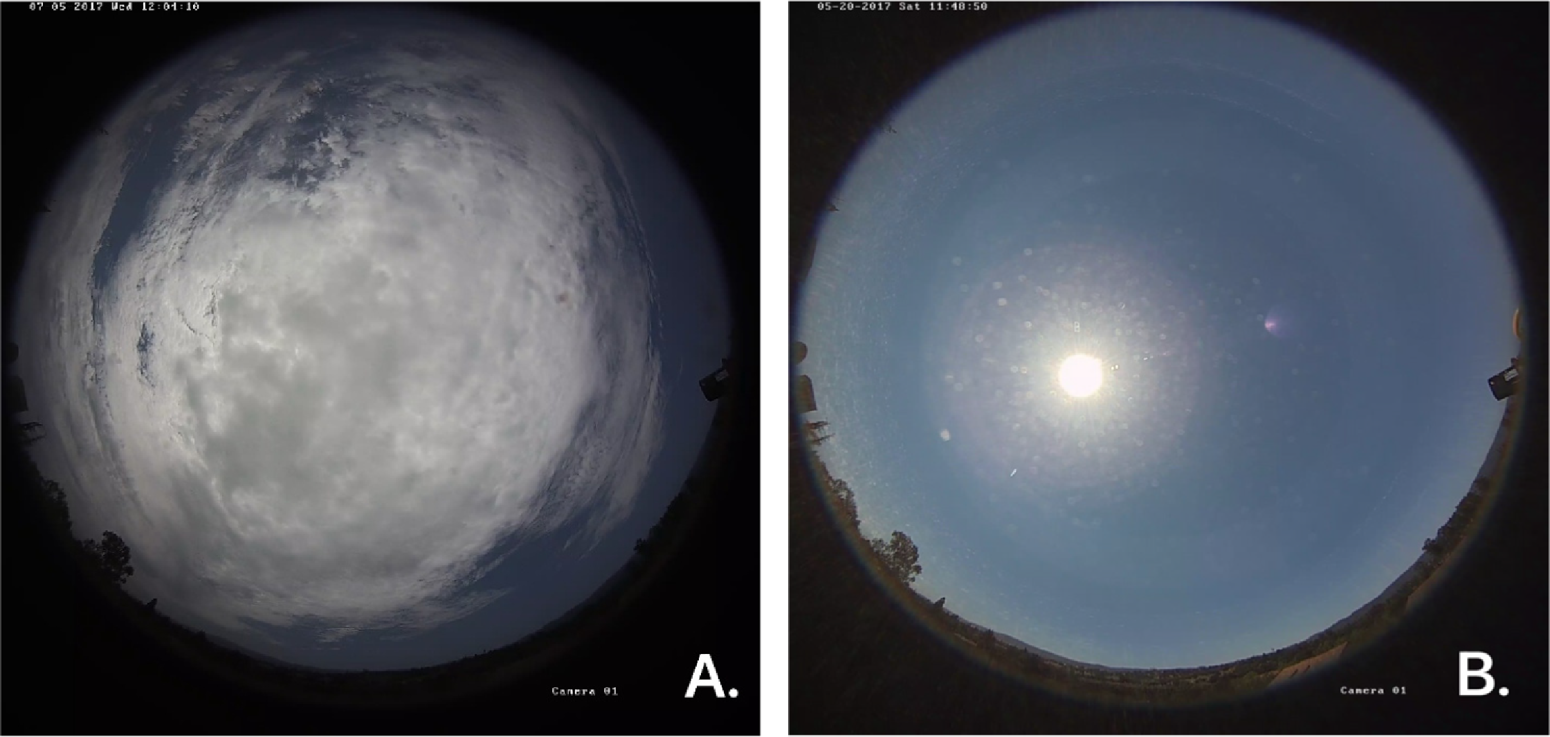
Figure 1: Sky images are illustrated as follows: (A) a cloudy sky captured on 05 July 2017, and (B) a sunny sky captured on 20 May 2017

3.1.2 PV Power

PV output data were obtained from a rooftop solar array located on the Jen-Hsun Huang Engineering Center at Stanford University, situated approximately 125 m from the sky camera—a distance negligible compared with typical cloud scales. Fig. 2 shows PV output examples under two different weather conditions. The installation consists of polycrystalline modules with a total capacity of 30.1 kW (DC), mounted at a tilt angle of 22.5° and oriented at an azimuth of 195°. Power output was monitored using a PowerLogic ION7330 m with an accuracy of ±0.5%, and the measurements were logged into the eDNA historian system at intervals ranging from one to ten seconds. Given the high precision and temporal resolution, measurement uncertainty can be considered negligible in the context of forecast error evaluation. For modeling purposes, the raw data were interpolated to produce second-by-second records and subsequently averaged into one-minute values, which served as both forecasting targets and model inputs.

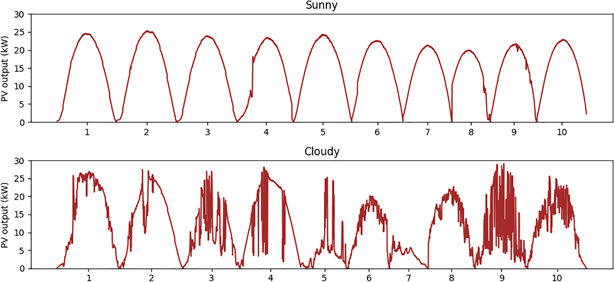
Figure 2: An example of data visualization for PV output data, which includes two different weather conditions: sunny and cloudy

3.2 Data Processing

To focus on the challenging periods for solar forecasting, only cloudy-sky samples were considered in this study, due to PV output under sunny conditions can be reliably predicted with physical models. Cloudy frames were identified using the algorithm of reference [9], which detects cloud pixels based on a modified red-blue ratio method. After filtering out sunny sky periods, a cloudy-sky subset containing 132,305 samples was obtained from the raw dataset.

For subsequent forecasting tasks, different input–output configurations were required. A common preprocessing procedure was therefore applied to build an interim dataset. Specifically, we traversed the cloudy dataset with a 2-min step size to ensure the availability of both historical and future records at one-minute resolution. This sampling frequency strikes a balance between training efficiency and model accuracy, as higher frequencies increase computational cost without clear performance gains. Samples with missing frames or incomplete PV measurements within the 30-min temporal window (15 min before and after the reference timestamp) were automatically excluded to guarantee continuity of the input sequence. After discarding incomplete samples, 60,385 valid sequences remained. Each sequence consists of 31 consecutive sky images and the corresponding PV measurements, spanning from 15 min before to 15 min after a given reference time.

From this interim dataset, task-specific datasets were constructed. For the image prediction task, only image sequences were used. Eight images from the past 15 min served as model inputs, while the subsequent eight frames (covering the next 15 min) were treated as prediction targets. For the PV output prediction task, two configurations were prepared. In the first setting (IP-U-Net dataset), a single sky image at time t was paired with the concurrent PV output value, enabling direct image-to-power regression. In the second setting (ACMCA dataset), sequences of sky images and PV outputs over the past 15 min were provided as inputs, and the PV output at t + 15 min was used as the prediction target.

In this study, the sky images were divided into two regions: the foreground, which represents the portion within the circular view captured by the camera, and the background, which is the area outside the circle. Although the background is black, its pixel values aren’t strictly zero but rather small values, likely due to sensor artifacts such as backscattering. While further verification is required, initial experiments suggest that these non-zero background pixels may still carry useful information for predicting PV output.

To focus our models on the more relevant foreground data, a binary mask was applied to the images, setting the background pixels to zero and the foreground pixels to one. This mask was utilized in two contexts: (1) When evaluating the performance of an image prediction model, the images generated by the model are masked, but the input images used for training are not masked; (2) during training, validation, and testing of the PV output prediction models, either real or generated sky images were masked in the same manner.

3.3 Data Partition

After preprocessing, the data were partitioned into training, validation, and test splits. For the validation set, we curated ten cloudy days from March 2017 to October 2019 so that seasonal and interannual variability were represented. The remaining records within this window were used for training. To assess out-of-period generalization, the test set comprises five cloudy days from November–December 2019, lying outside the training/validation window. Validation and test samples were never exposed to the models during learning to prevent overfitting. The final split contains 53,336 training instances (88%), 4467 validation instances (7%), and 2582 test instances (4%). The image prediction model is fit and tuned using only the training and validation splits, whereas the PV output predictor leverages all three datasets.

4  Methodology

This study targets short-term probabilistic solar power forecasting, with the goal of producing 15-min-ahead PV output intervals. To address limitations of current sky image approaches—namely insufficient cloud-evolution modeling and the lack of formal uncertainty characterization—we develop a two-stage short-term photovoltaic power forecasting framework. The first stage is a stochastic sky image prediction model that produces realistic and diverse future scenarios conditioned on past sky image frame. The second stage is an image-to-power regressor that converts those predicted frames into interval forecasts of future PV power. A schematic of the system appears in Fig. 3. For the mapping step, the regressor consumes only the final predicted frame, and historical power measurements are excluded to prevent the model from overfitting to recent trends.

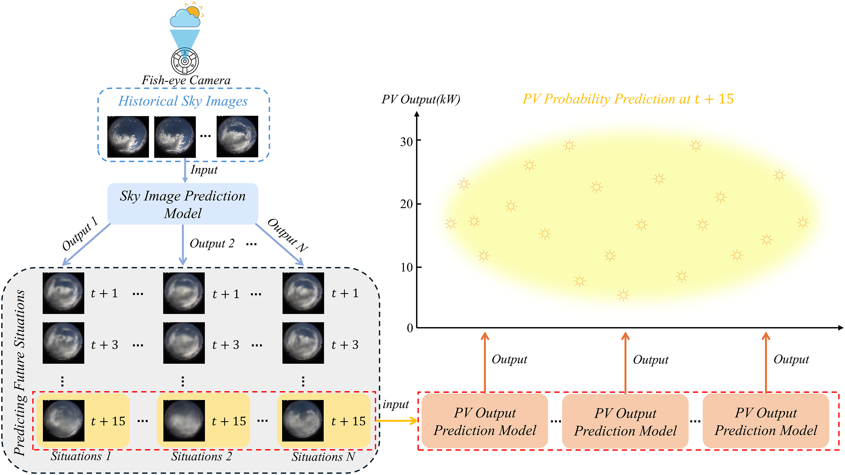
Figure 3: Proposed a novel two-stage ultra-short-term photovoltaic power forecasting framework

4.1 Sky Image Prediction

In this study, the problem of predicting future sky images is framed as a sequence-to-sequence forecasting challenge. The objective is to predict sky images for future time steps, starting at time point t + 1 and ending at time point t + 15, with each time point occurring at 2-min intervals. These predictions are made based on a sequence of past sky images captured from t − 15 to t − 1, also at 2-min intervals. To account for the inherent uncertainty, the model generates a variety of potential future sky scenarios by sampling distinct latent sequences from the prior distribution, learned during training. This approach enables the model to produce multiple plausible futures for the same set of input images. Fig. 4 shows the structure of the proposed I-GPT model.

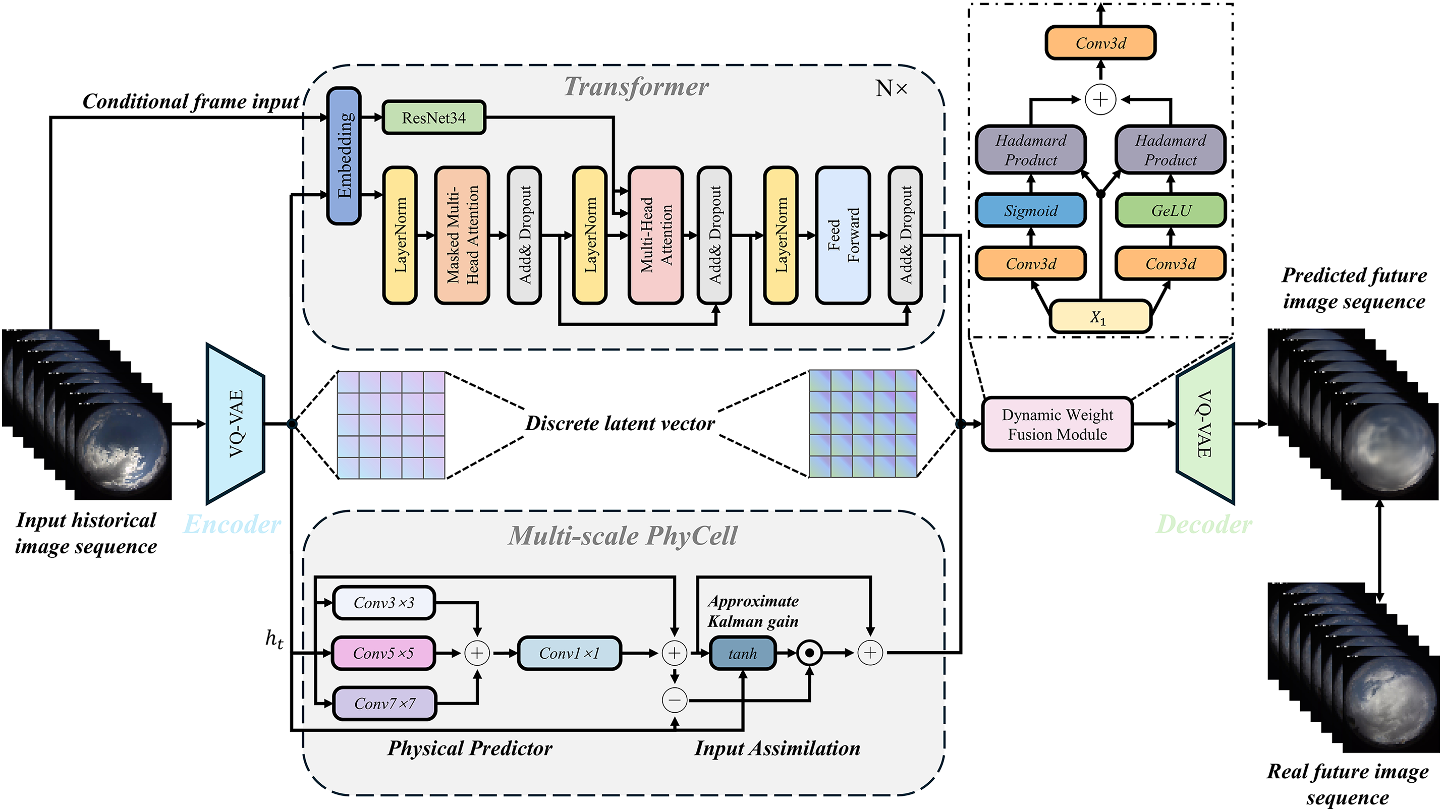
Figure 4: The model structure diagram of the proposed sky image prediction model I-GPT

Our image prediction model follows a two-stage module in the early stage: a vector-quantized variational autoencoder (VQ-VAE) [38] and an image transformer [39]. VQ-VAE follows an encoder and decoder design but learns a discrete latent space instead of a continuous one. Concretely, we first train the VQ-VAE model on the sky image data, which mainly learns a set of discrete latent encodings. Next, a series of 3D convolutions are stacked in the encoder. These convolutions are downsampled in both space and time, and the next part is the attention residual block. Each block uses LayerNorm [40] with axial attention layers [41,42] to capture long-range spatiotemporal dependencies at modest cost, design as shown in Fig. 5. Given an input clip x, the encoder outputs latent vectors h=E(x), which are quantized via a nearest-neighbor lookup in a learnable codebook C={ei}i=1K (with K controlling the number of prototypes); codebook entries are randomly initialized and updated during training. Learned spatiotemporal position embeddings are shared across the axial-attention layers in both encoder and decoder. The decoder and encoder employ a mirrored architecture, both utilizing attention-based residual blocks followed by 3D transposed convolutions to up-sample and reconstruct frames from quantized embeddings. We model future frames in the latent domain rather than at the pixel level: an autoregressive transformer predicts the next latent tokens by masking future positions and feeding back its own previous predictions. Working in this compact, downsampled space reduces redundancy in high-dimensional imagery while retaining long-range dependencies, and the discrete codes naturally capture different sky regimes (sunny, cloudy, overcast). To make the prediction conditional on a short history, frames from t − 15 to t − 1 are first summarized by a 3D ResNet; during training, the transformer cross-attends to this summary so that, at inference, diverse but plausible futures can be sampled from the learned conditional prior. Finally, the predicted latent tokens are decoded by the VQ-VAE to recover videos at the original resolution.

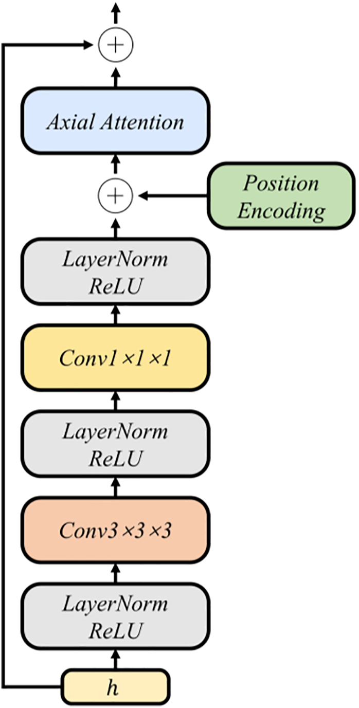
Figure 5: Structure diagram of attention residual block in VQ-VAE

We have added a new branch of physical guidance to incorporate the previous physical knowledge into the transformer, which is implemented as a Partial Differential Equation (PDE) constrained recursive cell called PhyCell to better capture the random motion of clouds. We employ a PDE-constrained recurrent cell that performs prediction–correction in the latent image-embedding space. During prediction, a bank of learnable derivative filters, trained under kernel-moment constraints, approximates spatial derivatives of multiple orders; their responses are linearly recombined through a 1 × 1 projection to form a compact surrogate of linear PDE dynamics, including advection–diffusion, heat, and wave processes. The correction step assimilates the current encoded observation by means of a Kalman-style gate computed from the predicted state and the observation via shallow convolutions with a bounded nonlinearity, producing a spatially varying confidence map that balances trust between the physical forecast and the data. To capture both thin, fast cloud filaments and broader mesoscale structures, we extend the PhyCell to a multi-scale design, called Multi-scale PhyCell, in which several convolutional stacks with different receptive fields, obtained by varying kernel size, stride, and dilation, produce scale-specific physical predictions that are learnably fused before assimilation. This integrated design promotes coherent, physically plausible advection, preserves sharp appearance details, and improves stability during long rollouts and under partial observation.

In parallel, the transformer pathway models fine-grained appearance through masked self-attention in the latent token space. At each time step, we do not fuse the physics and appearance embeddings by simple addition; instead, we employ a Dynamic Weight Fusion Module (DWFM), as shown in Fig. 6. DWFM takes the shared input features and processes them with two parallel 3D convolutional branches. One branch uses Gaussian Error Linear Unit (GELU) to extract rich nonlinear cues, while the other uses Sigmoid to generate an adaptive gating mask. The outputs of both branches are multiplied element-wise with the original features to perform content-aware filtering, producing two reweighted streams that emphasize informative structures and suppress irrelevant components. These filtered streams are then summed and passed through a final 3D convolution to yield the fused embedding, with a residual path preserved for stability. This dynamic weighting assigns data-driven importance to the physics and appearance cues, enabling the decoder to recover frames at the original resolution with sharper details, more coherent motion, and improved robustness under rapidly varying weather and partial observations.

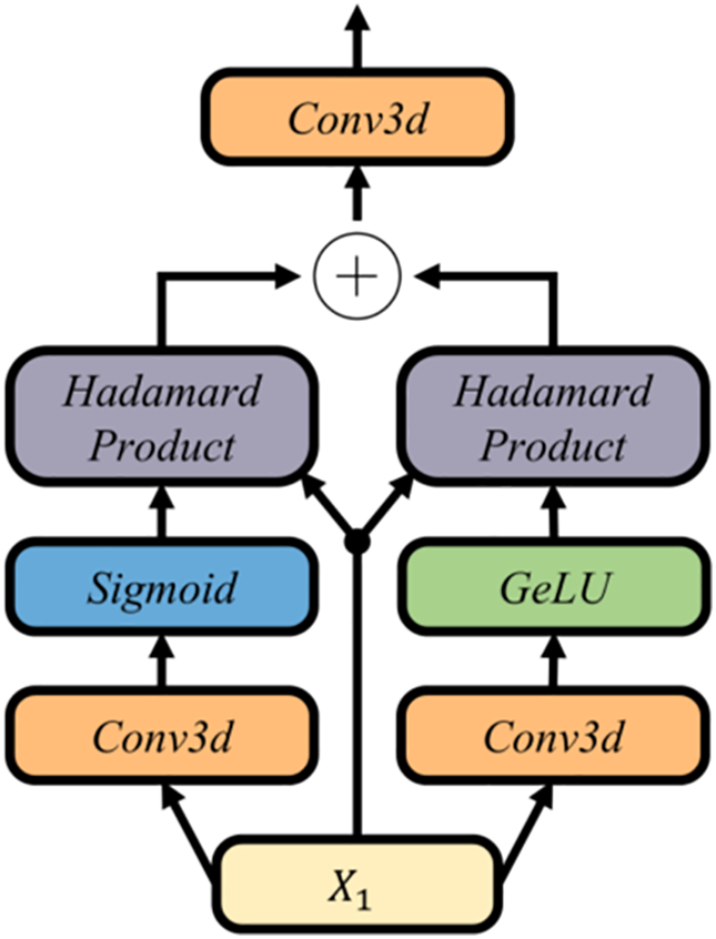
Figure 6: Schematic of the proposed dynamic weight fusion module

The calculation process of DWFM is described below:

O1=α(Coπν1(X1))⊙X1(1)

O2=β(Coπν2(X1))⊙X1(2)

Next, the merged activations O1 and O2 are fed into the final 3D convolutional layer Coπν3(⋅):

OutDWFM=Conv3(O1+O2)(3)

In this case, α designates the GELU activation as defined in Eq. (4), whereas β designates the Sigmoid activation in Eq. (5).

GELU(x)=12x(1+tanh⁡(2π(x+0.044715x3)))(4)

Sigmoid(x)=11+e−x(5)

4.2 PV Output Prediction

The second stage of our framework focuses on forecasting PV power output, formulated as a mapping problem from sky images to simultaneous PV measurements. This mapping is first learned from historical image–power pairs and subsequently applied to the synthetic future frames generated in the first stage. To this end, we designed a U-Net [43] model based on the encoder-decoder paradigm for converting sky images into PV outputs, which we refer to as IP-U-Net. While the classic U-Net model is widely used in image segmentation, we made several key modifications for its application in the image-to-PV value mapping regression task in this study. First, the network output was changed from segmentation masks to scalar regression values representing PV power. Second, the section between the encoder and decoder employs residual blocks instead of the traditional Conv-BatchNorm-ReLU module design, enhancing training stability and gradient flow. Third, we incorporate an Attention Gate module in the skip-connection between encoder and decoder. This effectively suppresses irrelevant background noise, enabling the decoder to focus on regions near the sun and high-contrast cloud edges. Fourth, we streamline the architecture by reducing the depth of convolutional layers, enhancing efficiency without sacrificing accuracy.

Fig. 7 shows the structural diagram of our proposed model. The encoder employs a two-dimensional convolutional stack to compress high-dimensional sky images into compact latent representations. This latent signal undergoes processing through residual blocks before being upsampled by the decoder. The decoder alternates between upsampling and 2D convolutions to restore spatial resolution. Meanwhile, skip connections between the encoder and decoder, when passed through the AG module, better suppress noise in irrelevant regions while focusing on cloud segments useful for prediction. This approach effectively recovers fine-grained spatial details lost during subsampling, further enhancing performance. Unlike standard U-Net, however, the output is not a reconstructed image but a single-channel feature map sharing the same spatial dimensions as the input, each location encodes its contribution to photovoltaic power generation. The final PV prediction is obtained as the weighted sum of this feature map. This model significantly improves prediction accuracy while enhancing interpretability by directly linking spatial features of the sky to PV power estimation.

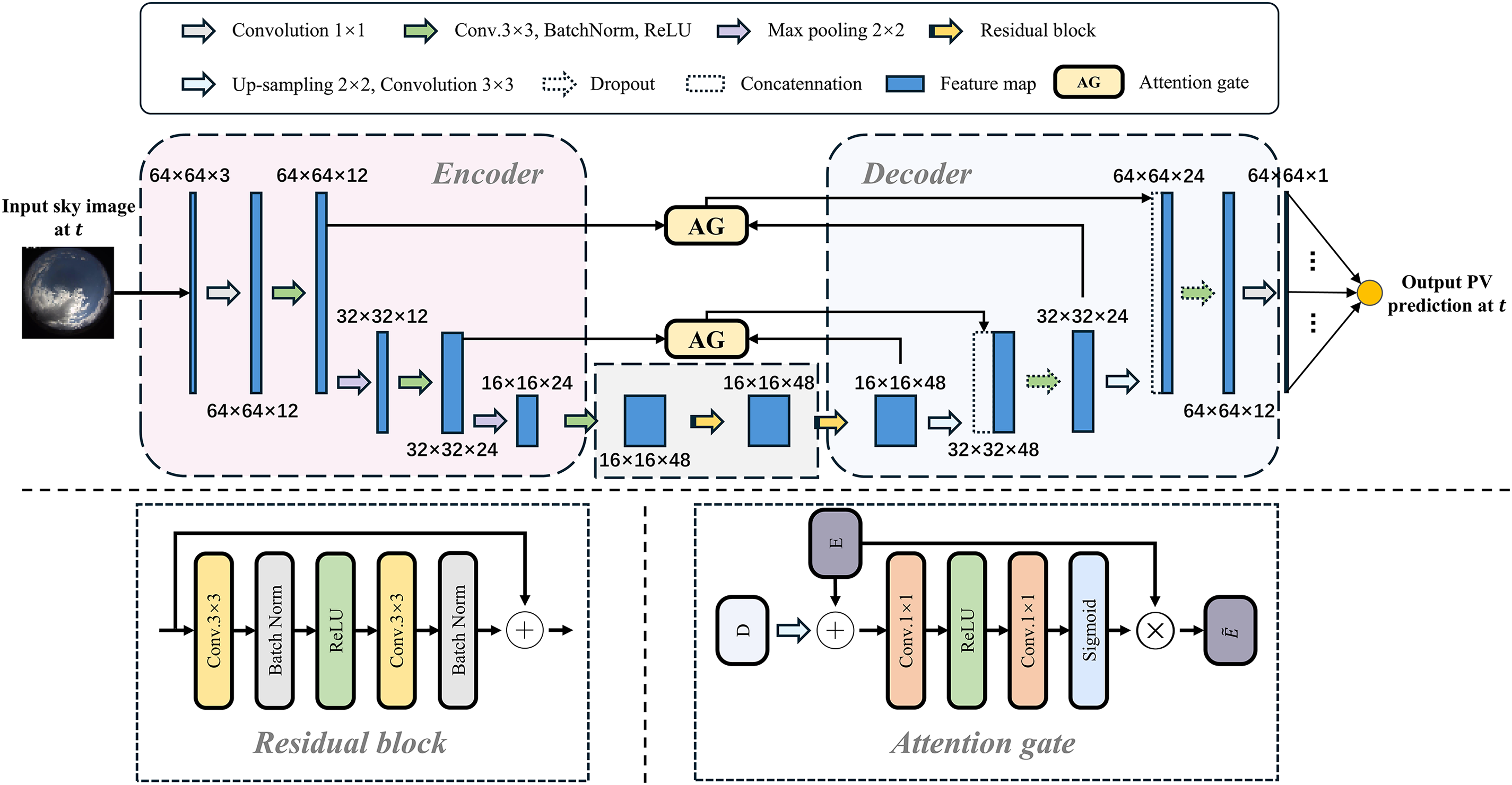
Figure 7: The model structure diagram of the proposed PV output prediction model IP-U-Net

4.3 Loss Function

4.3.1 Loss function of Sky Image Prediction

In this research of sky image prediction, the VQ-VAE part and the part composed of Multi-scale PhyCell and Transformer were trained respectively. First, the loss function of training VQ-VAE is as follows:

ℒVQ−VAE=ℒreconstruction+ℒcodebook+βℒcommitment(6)

where includes three loss functions: reconstruction loss ℒreconstruction, codebook loss ℒcodebook and commitment loss ℒcommitment.

•   Reconstruction loss (ℒreconstruction): Drives the decoder D(⋅) to accurately recover the input x from the quantized embeddings e, ensuring that the latent codes retain task-relevant information. Formula in Eq. (7).

ℒreconstruction=∥x−D(e)∥22(7)

•   Codebook loss (ℒcodebook): Pulls each codebook vector toward its paired encoder output E(x), improving encoder–code alignment and stabilizing the discrete assignment. Formula in Eq. (8).

ℒcodebook=∥sg[E(x)]−e∥22(8)

•   Commitment loss (ℒcommitment): Weighted by a hyperparameter β, penalizes encoder outputs that drift across code entries, encouraging the encoder to “commitment” to a selected code and preventing code-hopping. Formula in Eq. (9).

ℒcommitment=∥sg[e]−E(x)∥22(9)

where sg[⋅] is the stop-gradient operator. It structures gradient flow as follows: the decoder is updated only by the reconstruction loss; the encoder receives gradients from the reconstruction and commitment losses; the codebook embeddings are updated by the codebook loss. This separation is essential for stable optimization and for learning discrete, well-behaved latent representations.

The loss function of the training consisting of Multi-scale PhyCell and Transformer is as follows:

ℒMulti−PhyCell−transformer=ℒmoment+ℒcross−entropy(10)

where includes two loss functions: a moment loss ℒmoment and a cross-entropy loss ℒcross−entropy.

•   Moment loss (ℒmoment): To constrain the convolutional operators in the physics pathway to behave like spatial derivatives from a family of linear PDEs, we match their kernel moments to target moments. Formula in Eq. (11).

ℒmoment=∑i≤k∑j≤k∥M(wp,i,jk)−Δi,jk∥F(11)

where k denotes the convolutional kernel size; wk,i,jp is a learnable kernel parameter of the physical cell; M(⋅) computes the corresponding moment matrix; ∥⋅∥F is the Frobenius norm; and △i,jk is the target moment matrix for derivative order (i,j). In our Multi-scale PhyCell, the same constraint is applied at every scale and summed across scales, ensuring derivative behavior is consistent for different receptive fields.

•   Cross-entropy loss (ℒcross−entropy): Evaluate the Transformer’s ability to predict the next latent variable. Formula in Eq. (12).

ℒcross−entropy=∑i=1N∑j=1Cyilog⁡Pi,j(12)

where N denotes the number of tokens and C denotes the number of classes. The ground-truth label for token i is yi, expressed as a one-hot vector yi. The predicted probability that token i belongs to class j is Pi,j.

4.3.2 Loss Function of PV Output Prediction

In this research of PV output prediction. The proposed IP-U-Net is trained as a deterministic regressor by minimizing the MSE between measured and predicted PV power. The loss function formula is as follows:

MSE=1N∑i=1N(P^i−Pi)2(13)

where N is the number of training instances, P^i is the model’s estimate of PV output for sample i, Pi is the corresponding actual measurement value. This quadratic criterion penalizes larger deviations more heavily and drives the network to produce unbiased, variance-reduced scalar predictions for each input sky frame.

5  Experimental Setup

5.1 Evaluation Metrics

5.1.1 Evaluation Metrics of Sky Image Prediction

We assess the predicted frames both qualitatively (visual inspection) and quantitatively using three standard metrics: mean squared error (MSE), mean absolute error (MAE), and a perceptual similarity based on VGG cosine similarity (VGG-CS) [30]. Let I=RH×W×C be the reference image and I^=RH×W×C the prediction, where H,W,C denote height, width and channels. For a set of N samples indexed by k, and vectorized pixels indexed by i, The formula is as follows:

MSE=1N∑kN∑iH×W×C(Iik−I^ik)2(14)

MAE=1N∑kN∑iH×W×C|Iik−I^ik|(15)

For VGG-CS, we extract deep features vk=ϕ(Ik) and vk=ϕ(I^k) using a VGG-16 [44] network pre-trained on ImageNet. Features are extracted from the output of the penultimate max-pooling layer in VGG. Since VGG-16 expects 224 × 224 inputs, images are resized from 64 × 64 to 224 × 224 before feature extraction. The cosine similarity formula is as follows:

VGG−CS=1N∑kN(vk⋅v^k||vk||||v^k||)(16)

While MSE and MAE are widely used, they often reward over-smoothed predictions and do not always correlate with perceived quality. VGG-CS has been reported to align more closely with human judgment, so we report all three metrics for completeness and compare them on held-out samples.

For the sky image prediction model, we generate multiple rollouts for each historical sequence image rendering. In this experiment, we take 10 as examples, calculate VGG-CS according to the basic facts of each rollup, and select high-quality VGG-CS samples as representative predictions for calculating MSE, MAE and VGG-CS. This is also to evaluate whether the model can generate at least one credible future image for a given past sequence.

5.1.2 Evaluation Metrics of PV Output Prediction

A well-calibrated PV output forecast should exhibit two essential characteristics: its predictive distribution should align with the empirical distribution of the observations, that is reliability, and it should remain as concentrated as possible while still encompassing the realized outcome,that is sharpness. Accordingly, to enable a more comprehensive assessment, we employ in this experiment two metrics that jointly evaluate reliability and sharpness, namely the continuous ranked probability score (CRPS) [45] and the Winkler score (WS) [46].

•   Continuous Ranked Probability Score (CRPS)

For each case k, let Fmodelk(x) be the predictive cumulative distribution function (CDF) of PV output and let Ftargetk(x) be the empirical CDF that jumps from 0 to 1 at the observed value xk (i.e., a Heaviside step at xk). The CRPS averages the squared CDF distance:

CRPS=1N∑k=1N∫−∞+∞[Ftargetk(x)−Fmodelk(x)]2dx(17)

Lower values indicate better probabilistic accuracy. A useful property is that CRPS has the same units as the label variable; for deterministic forecasts it reduces to absolute error, enabling direct comparison between probabilistic and point predictions.

•   Winkler Score (WS)

For a nominal coverage level (1−α)%, let [Lk,Uk] denote the predictive interval and define its width δ=Uk−Lk. The per-case score is:

WSk={δifLk≤xk≤Ukδ+2(Lk−xk)/αifxk<Lkδ+2(xk−Uk)/αifxk>Uk}.(18)

We calculate the average WS across N predictions to evaluate the overall performance:

WS=1N∑kNwsk(19)

In our experiments, we set α=0.1 and construct the interval using the 5th and 95th percentiles, so that Lk and Uk correspond to a 90% nominal prediction interval. WS penalizes two failure modes simultaneously: observations that fall outside the interval, indicating lack of reliability and excessively wide intervals indicating a lack of sharpness. Consequently, smaller WS and smaller CRPS both indicate better-calibrated and more informative PV output prediction.

To compare our approach with established baselines, we report the forecast skill (FS) of each model with respect to a reference method. FS quantifies the fractional error reduction relative to the reference and is expressed as:

FS=(1−ErrorforecastErrorreference)×100%(20)

As reference we adopt the smart persistence model (SPM) widely used in solar forecasting. SPM assumes the clear-sky index—the ratio between real PV output and its clear-sky counterpart—remains constant over a short horizon t→t+T:

kc=P(t+T)Pc(t+T)=P(t)Pc(t)(21)

where kc denotes the relative output. P(⋅) is the measured PV power, and Pc(⋅) is the theoretical clear-sky PV output. Pc is evaluated from a clear-sky model using solar position (zenith and azimuth) and the PV array orientation (tilt and azimuth) [47]. The formula is as follows:

Pc(t)=PmaxAa{cos⁡εcos⁡χ(t)+sin⁡εsin⁡χ(t)cos⁡[ξ(t)−ζ]}(22)

where Pmax is the maximum solar irradiance (1000 W/m2), Aa is the effective PV area (24.98 m2), χ(t) and ξ(t) are the solar zenith and azimuth angles, ε and ζ denote the array azimuth (with tilt 22.5° and azimuth 195° in our setup). Angles are computed from standard solar geometry formulas.

Under the persistence assumption, the SPM forecast at horizon T is as follows:

P^(t+T)=P(t)Pclr(t)×Pc(t+T)(23)

For FS we use CRPS as the error measure. Because SPM yields a single deterministic value, its CRPS collapses to the mean absolute error (MAE):

MAE=1N∑i=1N|P^i−Pi|(24)

This protocol allows a consistent comparison between probabilistic forecasts via CRPS and the deterministic reference via MAE-equivalent CRPS, and FS reports the percentage improvement of each method over SPM.

5.2 Implementation Details

5.2.1 Implementation Details of Sky Image Prediction

In the sky image prediction module, training proceeds in two stages. First, we train the VQ-VAE; second, we train the parallel Multi-scale PhyCell Transformer module, in which latent token modeling is explicitly split into two branches. To preclude leakage of latent information from Multi-scale PhyCell branch to the Transformer, the token embedding at time t is fused only with the previous step’s Multi-scale PhyCell embedding; otherwise, the Transformer will learn information generated by the Multi-scale PhyCell in the first few frames it produces. Prior to training, all images are normalized to [−0.5, 0.5]. For the VQ-VAE, we initialize the embedding vectors and codebook via random restarts by replicating encoder latents. The VQ-VAE is trained on contiguous sequences spanning t − 15 to t + 15 at a 2-min stride (eight historical and eight future frames). Afterward, the trained VQ-VAE is frozen and used to convert sky image frames into latent sequences, which serve as inputs for learning the Multi-scale PhyCell and Transformer branches; the conditional history frames is summarized by a 3D-ResNet and injected through cross-attention during this stage.

All experiments are conducted on a workstation with 13th-Gen Intel R Core i7-13700K CPUs (3.40 GHz), 128 GB RAM, and NVIDIA GeForce RTX 4090 GPU (24 GB). The software stack is Python 3.8, PyTorch 2.0.0, Ubuntu 22.04, and CUDA 11.8. Both stages of I-GPT are trained with the Adam optimizer, learning rate 3e−4, batch size of 32, and training budget of 200K steps.

5.2.2 Implementation Details of PV Output Prediction

In the PV output prediction model, training data consist of paired actual sky images and their corresponding PV value. Optimization uses Adam [48] with a scheduled learning-rate decay. The formula is as follows:

lr=lr0×γ⌊epoch10⌋(25)

where lr0 = 2e−4 is the initial rate, γ = 0.5 controls the decay, and ⌊⋅⌋ denotes the floor operator. To guard against optimistic bias, we adopt 10-fold cross-validation, yielding ten sub-models. The network is trained deterministically with the MSE loss described earlier.

At inference time, to produce a distribution over the PV output 15 min ahead, the proposed IP-U-Net is evaluated on a set of candidate future sky frames at t + 15 generated by the sky image prediction model. The number of candidate futures, Nf, is treated as a hyperparameter and is chosen to balance accuracy and computational cost. Because each fold produces an independent regressor, a single input image yields 10 × Nf PV estimates, which together define the predictive range for the target time. Generating 10 future scenarios for all 2582 test samples and mapping them to probability predictions took approximately 3.5 h, equivalent to roughly 0.5 s per prediction sample. The peak GPU memory consumption of this model during inference is approximately 6 GB. This demonstrates the model’s full capability to meet the ultra-short-term forecasting demands of virtual power plants.

The proposed model contains approximately 63 million parameters, which is slightly larger than traditional deterministic models such as ConvLSTM, PhyDNet, and PhyDNet+GAN. However, compared with more recent stochastic models such as VideoGPT (≈58 million parameters) and SkyGPT (≈61 million parameters), our model exhibits similar computational complexity and training cost—about 24 GPU hours on a single RTX 4090 GPU—while achieving notably higher forecasting accuracy. This demonstrates that the performance improvement arises from architectural innovation rather than parameter scaling. These results confirm that the proposed approach achieves a balanced trade-off between model complexity, training efficiency, and real-time inference performance. In future work, we plan to further enhance edge-deployment capability through structural pruning and lightweight optimization techniques.

6  Results and Discussion

6.1 Phase 1: Proposed Sky Image Prediction Model

6.1.1 Proposed Sky Image Prediction Model

Within our two-stage framework, the first component is a sky image prediction model that conditions only on the preceding 15 min of frames and generate the next 15 min. The design pursues two goals: it seeks high predictive accuracy by learning cloud kinematics from the historical sequence, and it promotes diversity by generating multiple plausible continuations from the same context so that the intrinsic randomness of cloud motion is reflected—an ability that is valuable for downstream evaluation of possible PV outcomes. Prior studies on sky image forecasting [13,33] either exhibit pronounced blur at longer horizons due to limited cloud-dynamics fidelity, or emphasize deterministic predictions with little variation across samples. In this study, we develop a stochastic sky image prediction model, I-GPT, built from two complementary branches (see Fig. 4): a multi-scale physics dynamics branch that injects domain knowledge to improve motion realism, and a visual generation branch based on a Transformer prior that supports long-range content synthesis and sampling of diverse futures from the learned conditional distribution. Finally, the two branches are fully complementary and fused through the dynamic weight fusion module, and the generated diverse future sky images are finally obtained.

6.1.2 Comparison between the Proposed Sky Image Prediction Model with the Baseline Models

For qualitative analysis of the results, I-GPT was compared with several baseline sky image prediction models. The baseline models include deterministic models PhyDNet+GAN [32], PhyDNet [27], and ConvLSTM [25]; and stochastic models VideoGPT [31] and SkyGPT [32]. We chose two representative sequences from the validation split—which the models never accessed during training—capturing distinct 30-min cloud evolutions: a transitioning from partly cloudy sky to overcast sky, and a transitioning from partly cloudy sky to sunny sky. These scenarios cause significant fluctuations in photovoltaic power output and pose substantial challenges to virtual power plant operations. Result visualizations are shown in Figs. 8 and 9. For these two distinct scenarios, while all image prediction models can generally accurately determine the overall trend of cloud changes, their clarity and detail appear markedly different—such as in generated cloud textures, lighting, and shadows—which may be crucial features for phase two solar prediction. PhyDNet and generate clear image for short-term futures but produce increasingly blurred predictions as time extends, reflecting the averaging of different cloud movement possibilities. In contrast, the stochastic models VideoGPT, SkyGPT, and our I-GPT generate clearer, more detailed images than ConvLSTM and PhyDNet over extended periods. They even rival images produced by PhyDNet+GAN, which leverages a GAN framework to consistently generate high-fidelity images but exhibits limited diversity in future outcomes. Overall, I-GPT demonstrates slight advantages over VideoGPT and SkyGPT in terms of overall lighting, shadow rendering, and image quality.

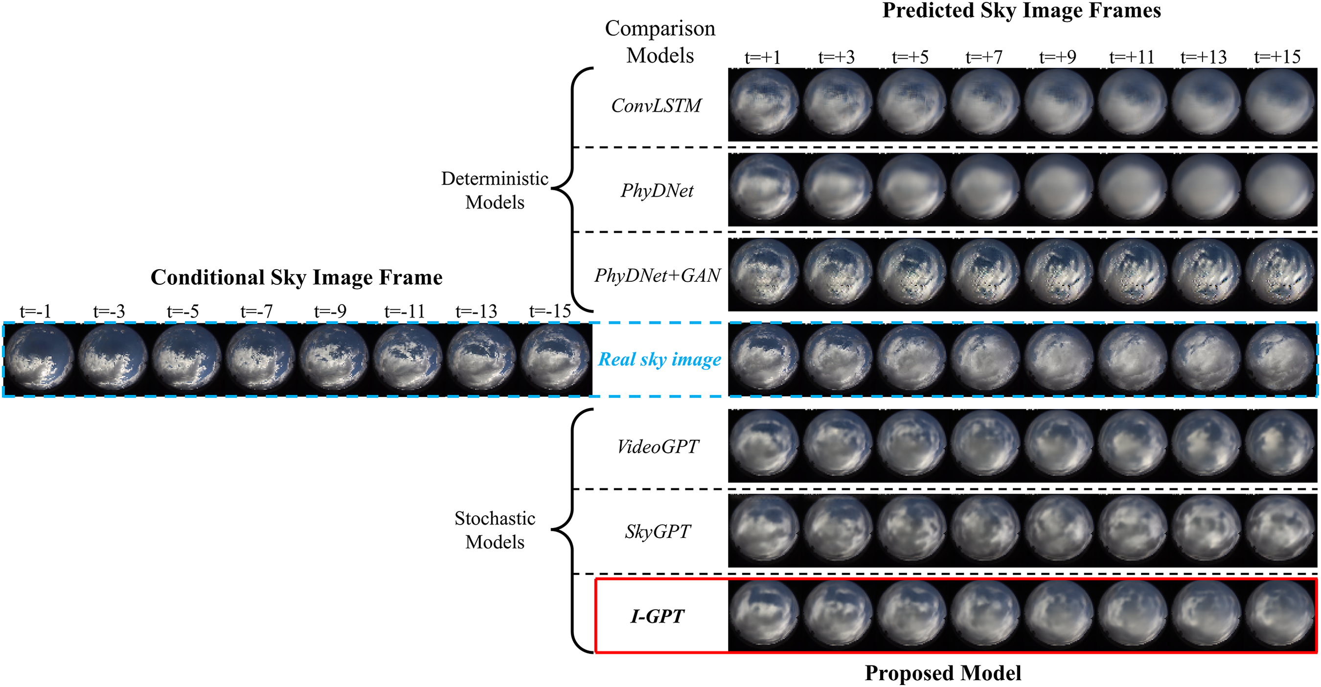
Figure 8: Future sky images generated by various models under partly cloudy sky to overcast sky conditions

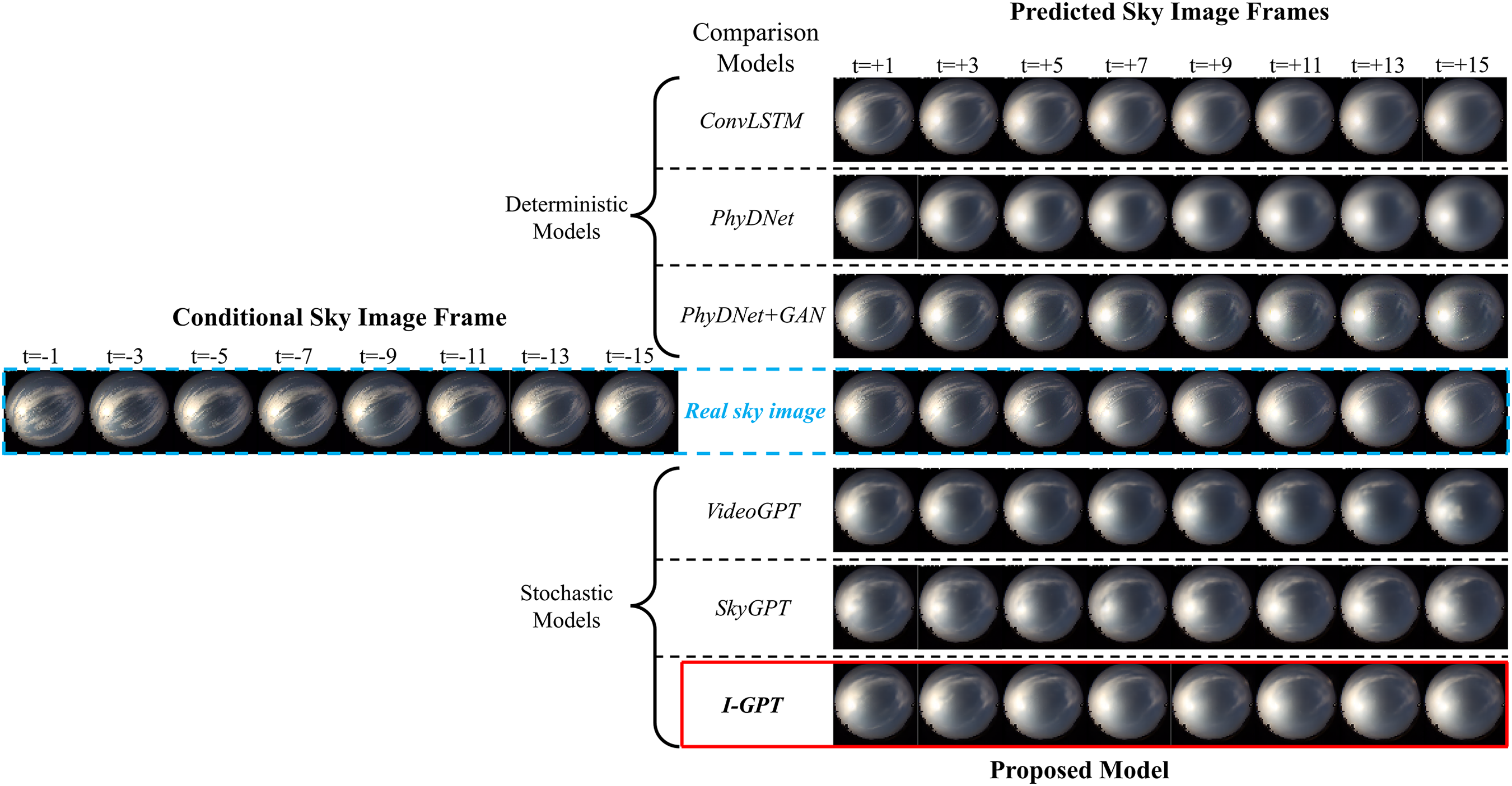
Figure 9: Future sky images generated by various models under partly cloudy sky to sunny sky conditions

These visual differences have direct consequences for downstream PV forecasting. When the predicted frames faithfully capture cloud-edge sharpness and the timing and extent of solar-disk occlusion—as reflected by spatial brightness gradients and shadow continuity—The model in the second stage will produces timely and correctly scaled power ramps. Conversely, blurred textures or misplaced illumination tend to underestimate rapid irradiance drops and induce phase-lagged recovery.

For quantitative analysis of the results, we rely on three commonly used performance metrics: MAE, MSE, and VGG-CS. We further quantified the accuracy of these models’ generated images using validation set comprising 4467 samples. Fig. 10 illustrates the relationship between the accuracy of predicted sky images from all image prediction models and the prediction time step length. As shown in the results figure, all three metrics decrease as the number of time steps increases. The baseline models PhyDNet and ConvLSTM often exhibit lower MSE and MAE than model PhyDNet+GAN, VideoGPT, SkyGPT, and I-GPT, despite generating blurrier images. This occurs because PhyDNet and ConvLSTM minimize MAE and MSE in various ways when training the model. As pixel-level metrics, MSE and MAE cannot understand the similarity of advanced image features, instead producing blurry predictions to align with the real sky image. However, over time, our I-GPT demonstrates lower MSE and MAE than ConVLSTM and PhyDNet. This fully demonstrates the predictive capability and potential of I-GPT. In contrast, VGG-CS exhibits superior image perception capabilities, yielding more photorealistic images generated by PhyDNet+GAN, VideoGPT, SkyGPT, and I-GPT—particularly when projecting into the distant future. Notably, these models significantly outperform ConvLSTM and PhyDNet when time steps exceed 5 min. Crucially, we observe that I-GPT’s VGG-CS degradation rate is markedly slower than that of PhyDNet+GAN, VideoGPT, and SkyGPT. Despite an initial disadvantage, it rapidly overtakes them to achieve a significant late-stage advantage. This further demonstrates I-GPT’s potential for long-term prediction and its accuracy.

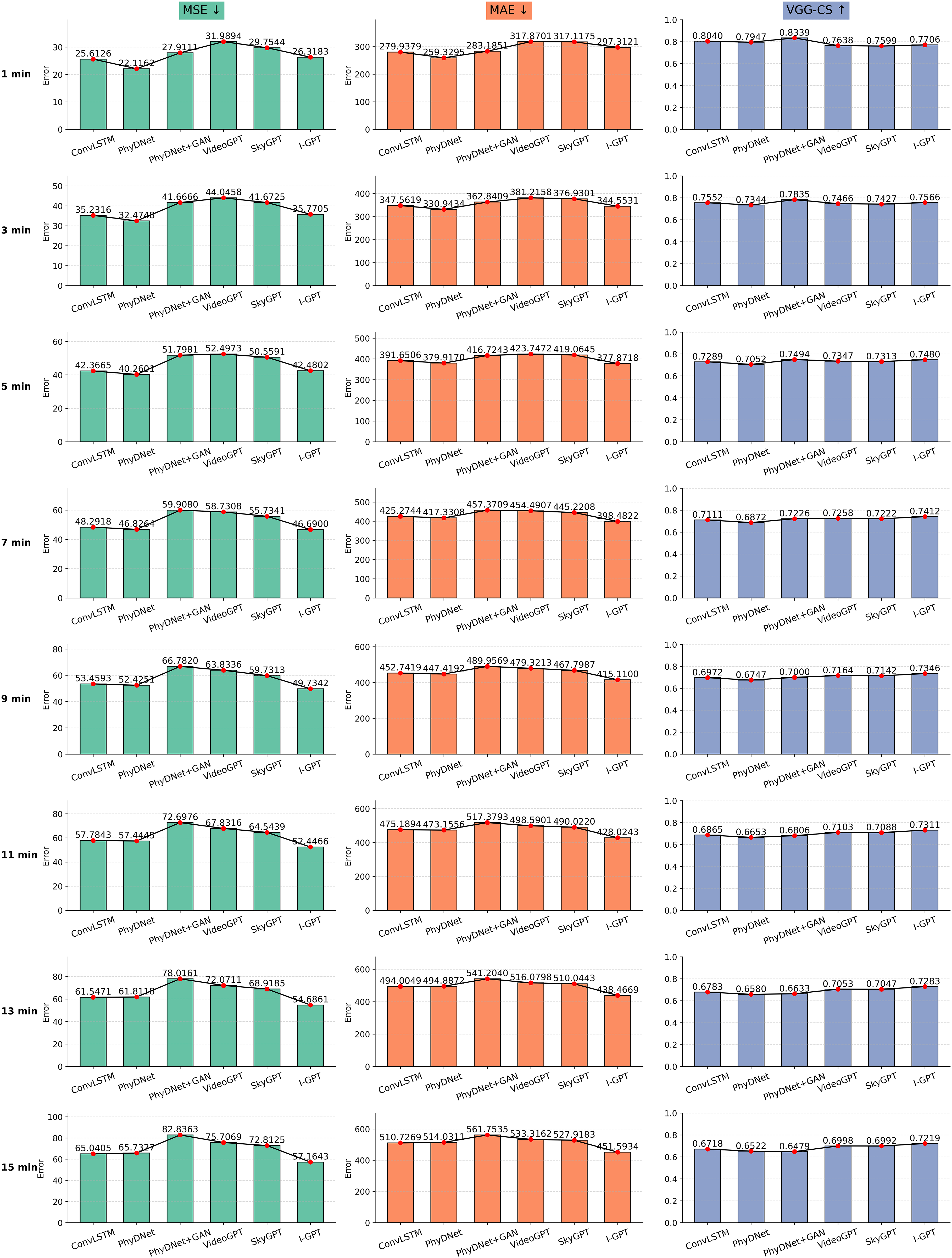
Figure 10: Visualization of quantitative results analysis of images generated by various models

The gradual degradation of pixel-wise metrics MAE and MSE with increasing forecast horizon implies growing spatial uncertainty in cloud representation, which in turn propagates to irradiance and PV prediction errors. In contrast, the slower decline in VGG-CS indicates that I-GPT better preserves high-level structural and brightness features related to solar-disk visibility and cloud thickness. These visually coherent patterns allow the the model in the second stage to maintain more consistent power estimates over longer horizons, particularly during transient cloud transitions. Thus, the superior perceptual stability of I-GPT’s generated images directly contributes to its improved probabilistic PV forecasting accuracy.

6.1.3 Generation Diversity of the Proposed Sky Image Prediction Model

We also selected two distinct weather conditions, feeding our model historical sky image sequences to generate ten sampled future sky scenarios, demonstrating the generative diversity of our proposed model. The results are shown in Figs. 11 and 12. We observe that during the initial few time steps, the cloud trajectories in these generated examples often exhibit similar patterns. However, as time progresses, these trajectories gradually diverge. In the example transitioning from partly cloudy sky to overcast sky conditions, clouds primarily drift from the lower left corner to cover nearly the entire frame. Most examples from our proposed stochastic model demonstrate this same drifting trend, fully showcasing the model’s robust predictive capability. Similarly, in examples transitioning from partly cloudy sky to sunny sky, clouds gradually dissipate from discrete, extensive coverage toward near-sunny conditions. Most examples generated by our proposed stochastic model exhibit the same decay trend. Certainly, some specific cloud changes are physically plausible—such as shifts in wind direction—though these may not align with the motion patterns learned from the data. However, our proposed model exhibits greater consistency with observed dynamics due to constraints imposed by our multiscale physical model. As prediction time steps advance, the divergence among random future scenarios grows increasingly pronounced, further validating our model’s robust generative diversity.

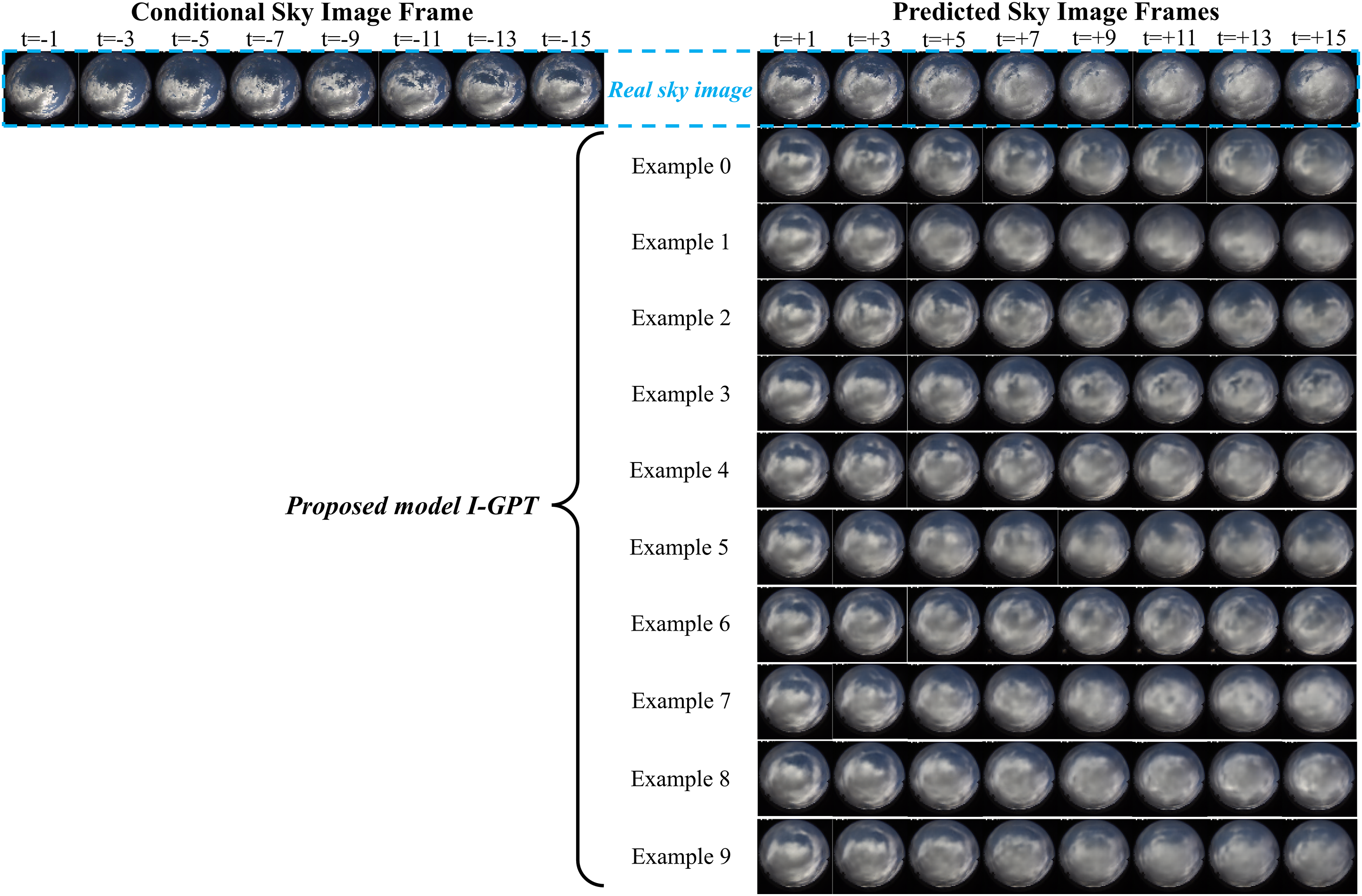
Figure 11: Visualization of qualitative results analysis of our proposed I-GPT model in partly cloudy sky to overcast sky conditions

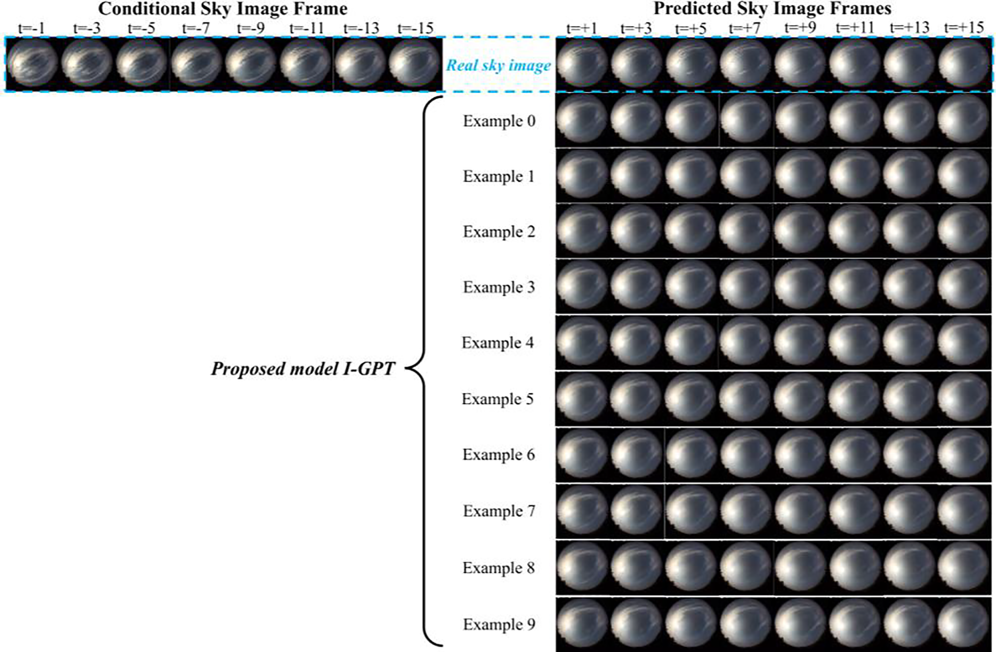
Figure 12: Visualization of qualitative results analysis of our proposed I-GPT model in partly cloudy sky to sunny sky conditions

This diversity also provides direct benefits for probabilistic PV forecasting. By generating mul-tiple physically plausible future sky scenarios, the model captures the inherent uncertainty of cloud advection and dissipation, which translates into a realistic distribution of possible irradiance and power trajectories. Scenarios exhibiting faster cloud accumulation correspond to lower predicted PV outputs, while those showing quicker cloud clearance lead to higher generation estimates. The ability to represent such a range of outcomes enables more reliable prediction intervals and sharper uncer-tainty bounds in the second-stage model. Consequently, the generative variability of I-GPT not only demonstrates physical realism but also enhances the robustness and interpretability of downstream PV forecasts under rapidly changing sky conditions.

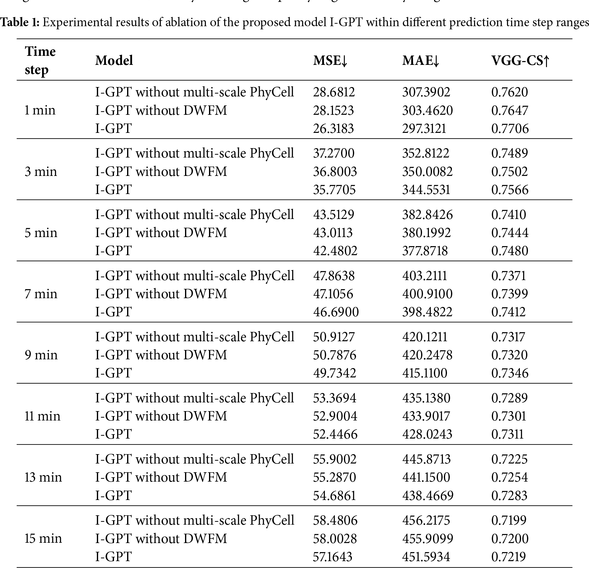
6.1.4 Ablation Experiments for the Proposed Sky Image Prediction Model

To elucidate the functionality of each component within the proposed I-GPT model, this section presents ablation results for different modules across various time step ranges from 1 to 15 min. It should be noted that all ablation experiments were performed using cloudy sky samples, as sunny sky conditions were excluded during preprocessing to focus on complex and highly dynamic cloud evolution scenarios. “I-GPT without Multi-scale PhyCell” refers to the model with the Multi-scale PhyCell module removed. “I-GPT without DWFM” refers to removing the Dynamic Weight Fusion Module at the end of the two prediction branches, replacing it with direct summation fusion. The ablation results are shown in Table 1. For each time step, removing the Multi-scale PhyCell module reduces the sky image prediction model’s ability to impose physical constraints on cloud changes, leading to a significant decline in generated image accuracy. Removing the final dynamic weight fusion module weakens the model’s capacity for effective feature extraction and mutual coupling of information between the two prediction branches, particularly during weather fluctuations, thereby affecting the quality of generated sky images.

6.2 Phase 2: Proposed PV Output Prediction Model

6.2.1 Proposed PV Output Prediction Model

The second component is the PV output prediction model. We utilize future sky image frames generated by our I-GPT and other baseline image generation models as input to our proposed IP-U-Net for PV probability prediction in this part. In this study, we employed the dataset introduced in Section 3 for a 15-min interval forecasting task. In renewable-rich virtual power plants, interval forecasts are more informative than point estimates because they convey the predictive uncertainty required for risk-aware decision-making.

For the second-stage probability prediction, the prediction interval is constructed through multi-point prediction. This is achieved by feeding each predicted frame from the first stage at t + 15 into the PV output prediction model as input. The PV output prediction model is an innovative U-Net architecture we developed, termed IP-U-Net. It was pre-trained on real-world sky image data spanning nearly three years, paired with concurrent PV output values. This model learns a direct mapping from sky images to scalar PV outputs, analogous to an image-to-numerical regression task. For deterministic sky image prediction models like ConvLSTM, PhyDNet, and PhyDNet+GAN, each input history generates a single future; however, we evaluate 10 IP-U-Net submodels generated via 10-fold cross-validation, yielding 10 PV prediction results. For stochastic sky image prediction models like VideoGPT, SkyGPT, and our approach I-GPT, we generate ten distinct future outputs for each history and feed them into ten IP-U-Net submodels. This yields 100 PV point predictions per scenario, from which we derive prediction probability intervals.

To benchmark our two-stage forecasting framework, illustrated in Fig. 3, we employed three baseline models for comparison. First is the Smart Persistence Model (SPM), a widely used standard comparison model in photovoltaic forecasting tasks—assuming the Clear Sky Index (CSI), defined as the ratio of actual PV output to its theoretical clear-sky counterpart, remains constant over 15 min. Second is a multimodal forecasting model that combines historical sky images with corresponding PV data for prediction. We also treat this as a baseline model in this section, referring to it as ACMCA [49]. It ingests 15-min historical sky image sequences at a two-minute resolution alongside PV measurements from t − 15 to t, without access to any future information. It is trained on the same dataset as our proposed IP-U-Net, with preprocessing adjusted to accommodate the hybrid input format. Finally, our IP-U-Net model shares the exact architecture with our proposal, differing only in its second stage: it is driven by the actual sky image frame at time t + 15 rather than the generated sky image frame from the first stage. This serves as the upper bound for a perfectly accurate sky image prediction model. Regarding outputs, SPM provides a single-point prediction at each timestamp, while ACMCA and IP-U-Net generate 10 predictions through their respective 10-fold cross-validation.

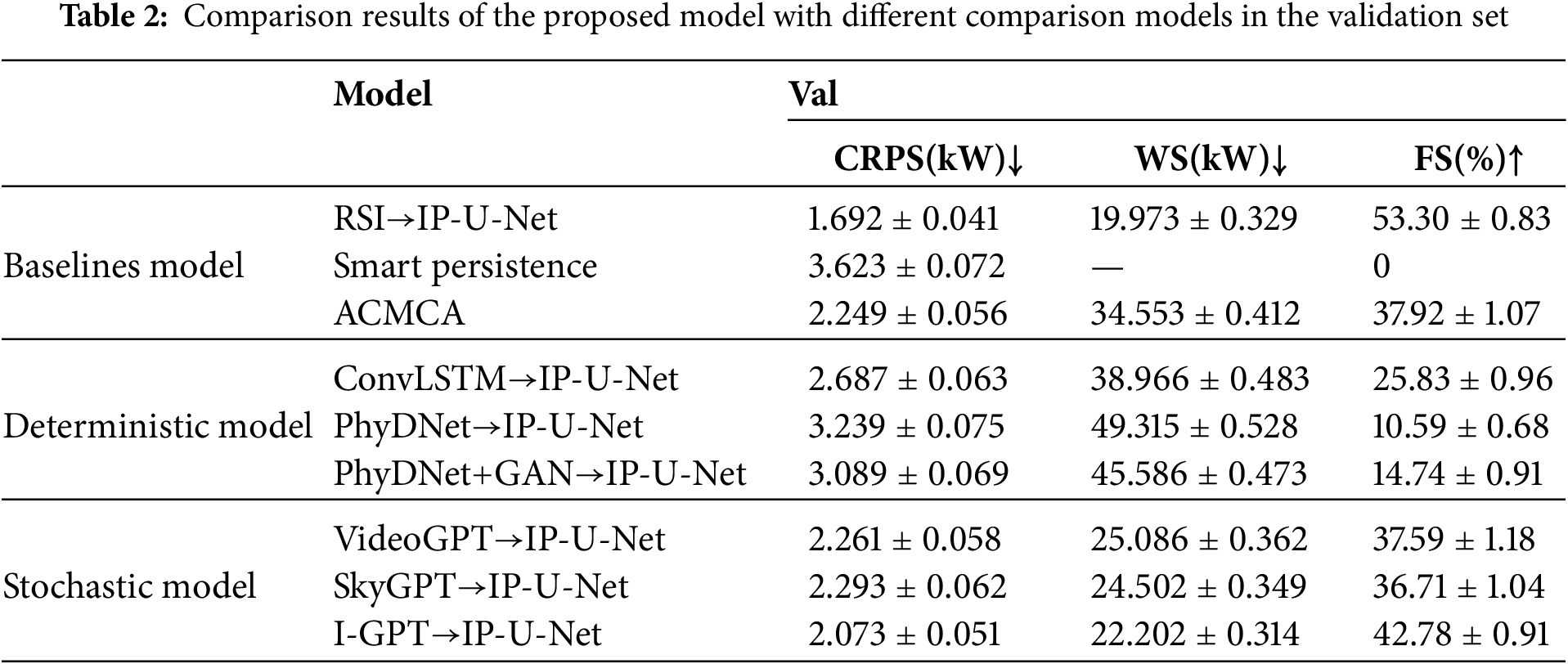
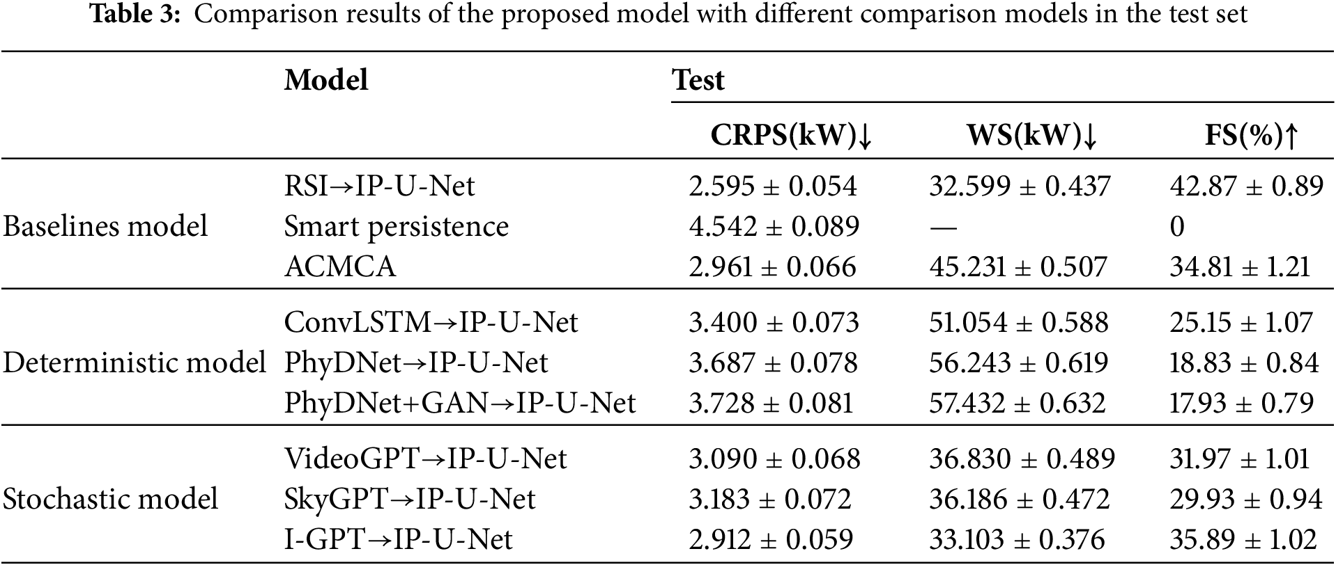
To validate the robustness of our proposed model, we conducted evaluations on two disjoint datasets: a validation set comprising 4467 samples randomly selected from 10 overcast days across the entire dataset, and a test set comprising 2582 samples randomly selected from 5 overcast days during November to December 2019. No grouping was employed during training. Probabilistic performance is summarized by the Continuous Rank Probability Score and the Winkler Score. Together, these metrics capture reliability—the empirical coverage of observations—and sharpness—the narrowness of intervals. CRPS measures the discrepancy between predictions and empirical cumulative distributions, while WS combines interval width with penalties for observations outside the central interval. Thus, lower CRPS and WS values indicate better calibration and greater informational gain. To compare with a widely used reference, we also report the predictive skill relative to SPM (FS), which quantifies the percentage error difference relative to the persistent baseline for each method.

6.2.2 Comparison between the Proposed PV Output Prediction Model with the Baseline Models

For quantitative analysis of the results, we validated the predictive performance of these models on the validation and test sets using CRPS, predictive skill relative to SPM (FS), and Winkler scores, as detailed in Tables 2 and 3. We observe that all comparison models outperform the intelligent persistence baseline model, achieving FS gains of 10.59% to 42.78% on the validation set and 17.93% to 35.89% on the test set. Our proposed I-GPT→U-Net pipeline achieves the strongest overall performance. Compared to the multimodal baseline model ACMCA, the two-stage prediction method consistently achieves lower WS, especially when using a random sky image prediction model. However, this is expected: sampling multiple candidate futures increases the chance that the prediction interval covers the actual sky state. In contrast, for CRPS and FS, the two-stage prediction method does not consistently outperform ACMCA and shows significant variability: for future images generated by the sky image prediction model, the FS range on the validation set spans from −27.33% to +4.86%, while the FS range on the test set was −16.88% to +1.08%. This not only demonstrates ACMCA’s exceptional predictive capability but also highlights the impressive predictive power and potential of I-GPT. The VideoGPT→U-Net and SkyGPT→U-Net combinations achieved respectable CRPS values on both validation and test sets (2.261 and 3.090 kW; 2.293 and 3.183 kW, respectively), yet still fell short of I-GPT’s performance. In contrast, our I-GPT→U-Net demonstrated the best stability and generalization capability, achieving 2.073 kW (FS 42.78%) on the validation set and 2.912 kW (FS 35.89%) on the test set. Collectively, these findings suggest that while the three top-performing random sky image prediction models all incorporate Transformer-based prior knowledge, prediction models enhanced with multi-scale physical constraint components can further boost generalization capabilities under limited training data.

For the qualitative analysis of results, we selected three overcast days from both the validation and test sets, focusing on the 9:00–16:00 period for 15-min-ahead forecasts. The prediction curves for each model are shown in Figs. 13–18. Figs. 13–15 display the prediction curves for the baseline model, deterministic prediction model, and stochastic prediction model within the validation set. Figs. 16–18 present the prediction curves for the baseline model, deterministic prediction model, and stochastic prediction model within the test set. We defined two prediction intervals here: the light orange band marks the 5th–95th percentiles (nominal 90% coverage), while the dark orange band marks the 25th–75th percentiles (50% coverage). We observe that the ACMCA baseline model often lags behind peaks and troughs—particularly evident on the second day of both the validation and test sets—indicating suboptimal performance in handling ramp events. However, it maintains relatively accurate predictive capability for the remaining portions. Secondly, its prediction bands remain narrow, likely due to its reliance on fixed 16-frame historical sky images and PV values for forecasting, coupled with limited diversity across its 10 cross-validated submodels. In contrast, the pipeline directly mapping images to PV via IP-U-Net demonstrates superior handling of ramping issues. However, among these deterministic sky image prediction models, its generated diversity falls short of the baseline model. This conclusion is evident from the two distinct prediction range distributions, particularly pronounced on the second day of the test set. They perform moderately on days with high variability: while median predictions adequately capture ramp events, prediction ranges frequently fail to encompass the actual data curve. When driven by random sky image prediction models, IP-U-Net achieves significantly improved ramp coverage, with median trajectories tending to center within the observed variability range. As expected, the interval adapts to state changes—narrowing during static periods and widening when PV output becomes highly variable. Moreover, our I-GPT model outperforms the other two models in both ramp handling and diversity-accuracy tradeoffs, particularly on the first and second days of the validation set. This fully demonstrates the robust capability and potential of our proposed model for addressing such forecasting challenges.

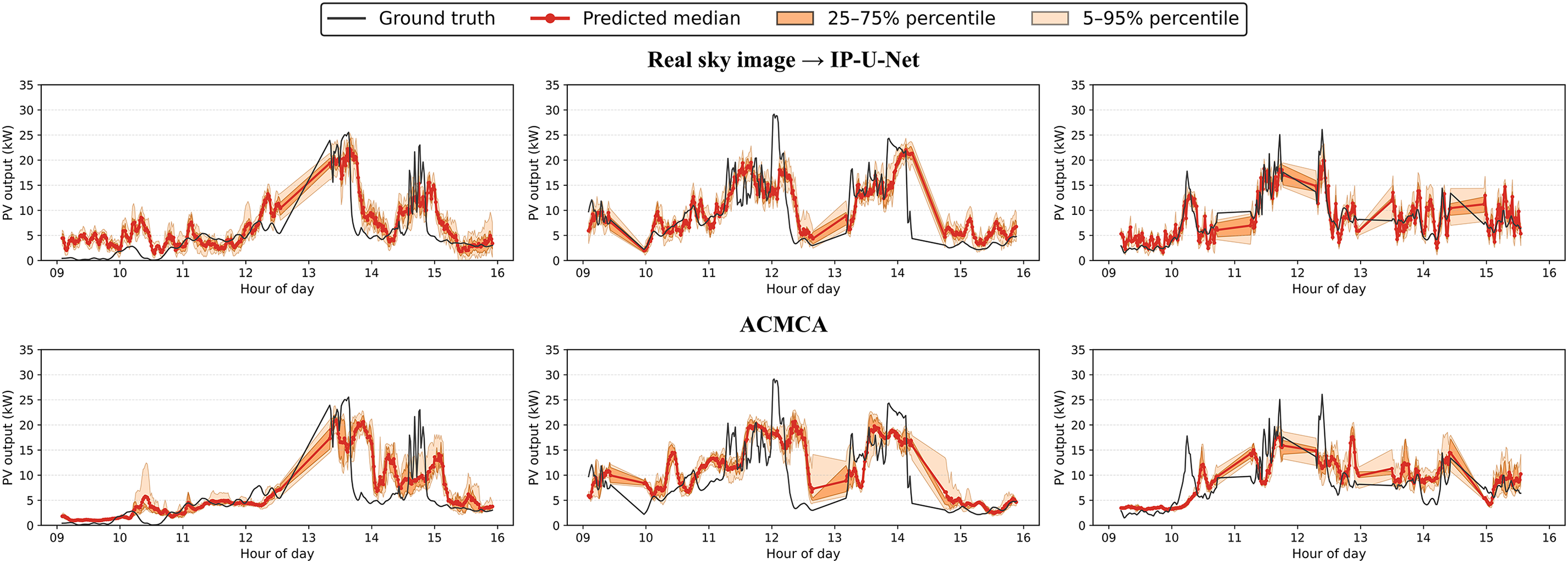
Figure 13: Visualize the prediction curve results of the baseline prediction model under 3 cloudy conditions in the validation set

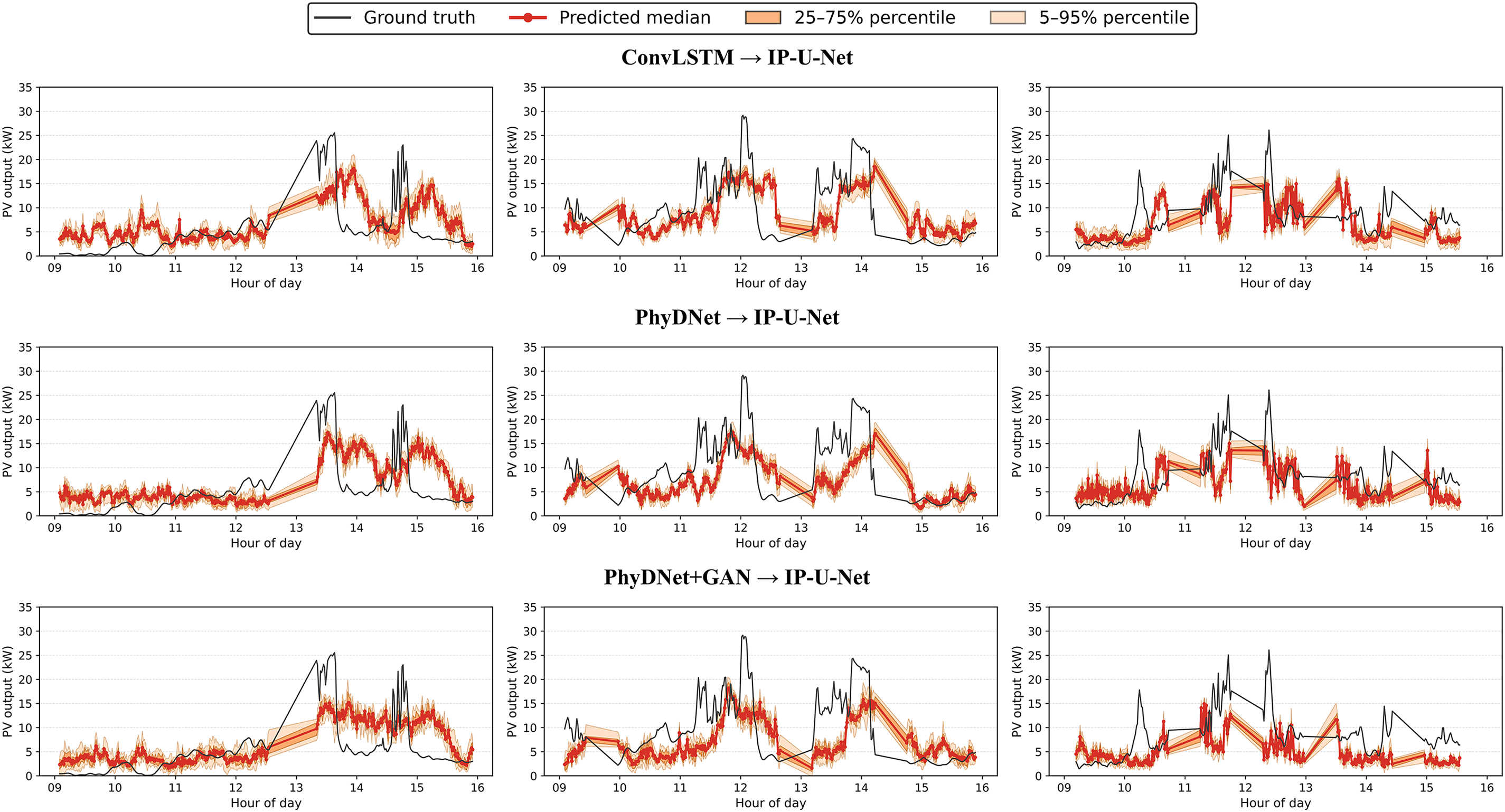
Figure 14: Visualize the prediction curve results of the deterministic prediction model under 3 cloudy conditions in the validation set

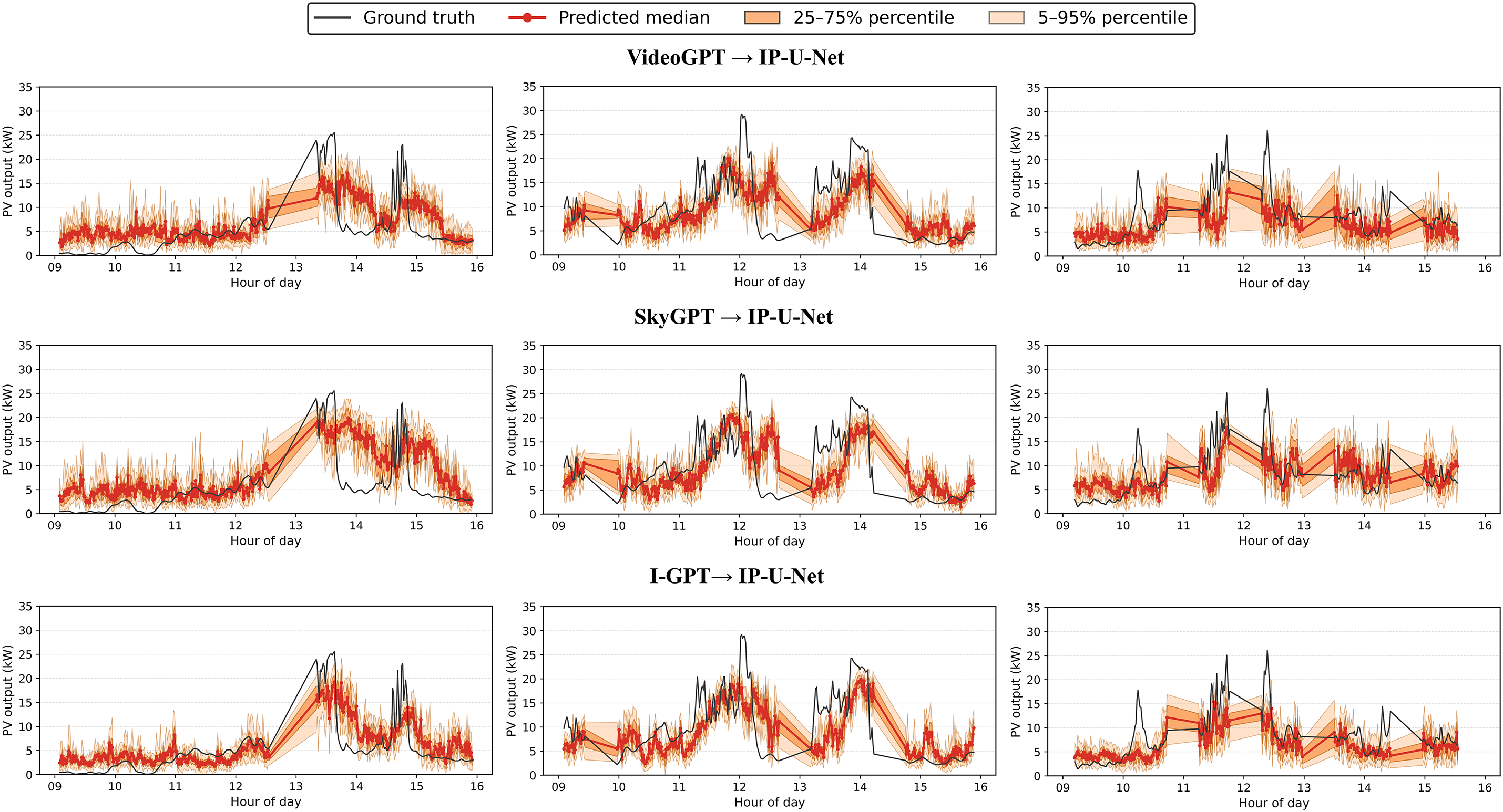
Figure 15: Visualize the prediction curve results of the stochastic prediction model under 3 cloudy conditions in the validation set

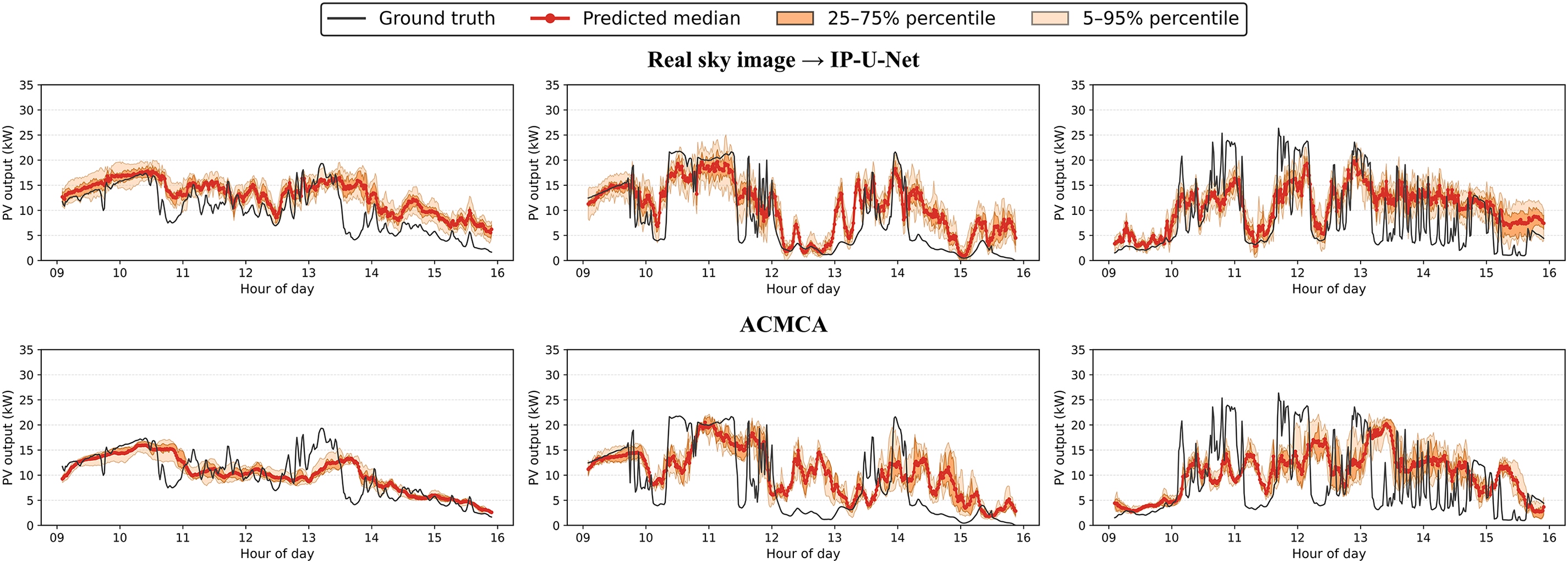
Figure 16: Visualize the prediction curve results of the baseline prediction model under 3 cloudy conditions in the test set

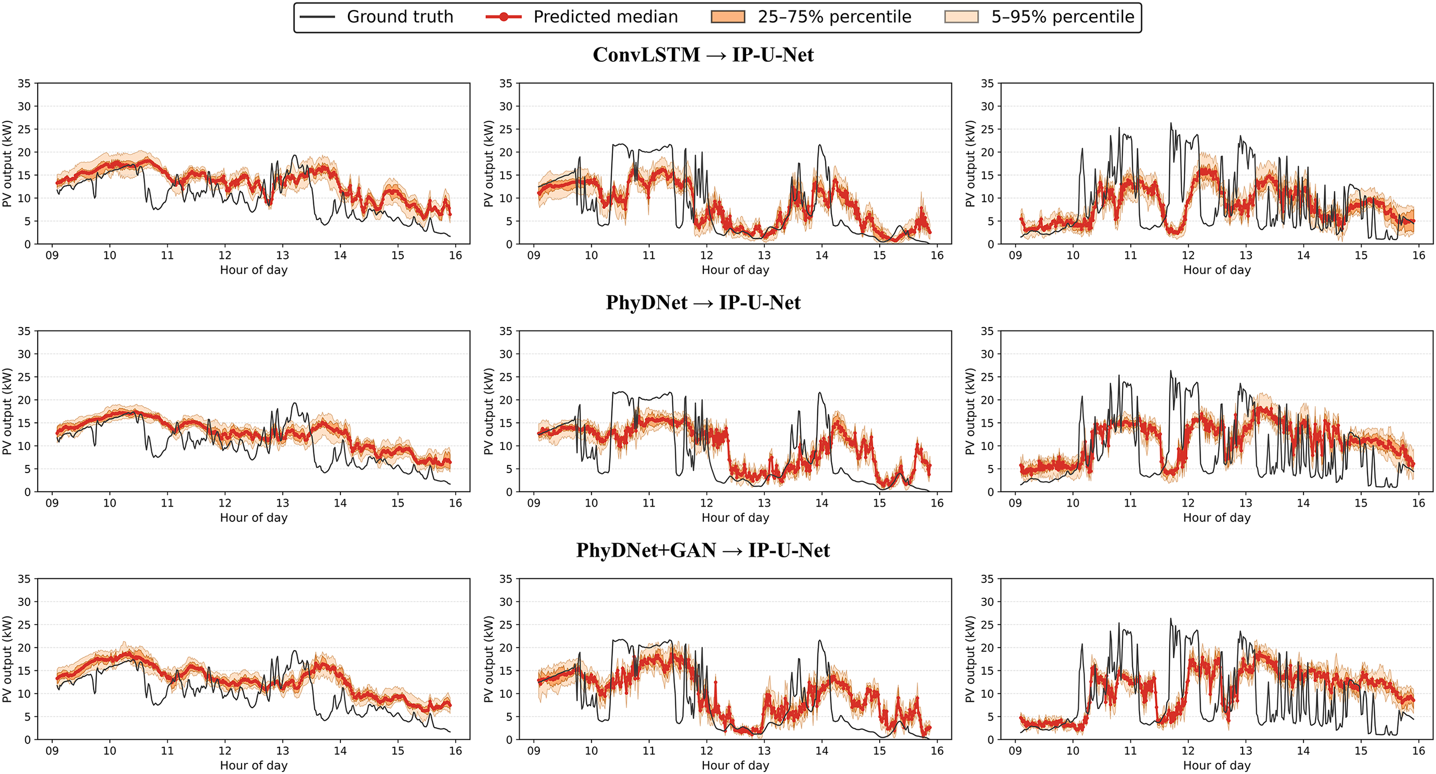
Figure 17: Visualize the prediction curve results of the deterministic prediction model under 3 cloudy conditions in the test set

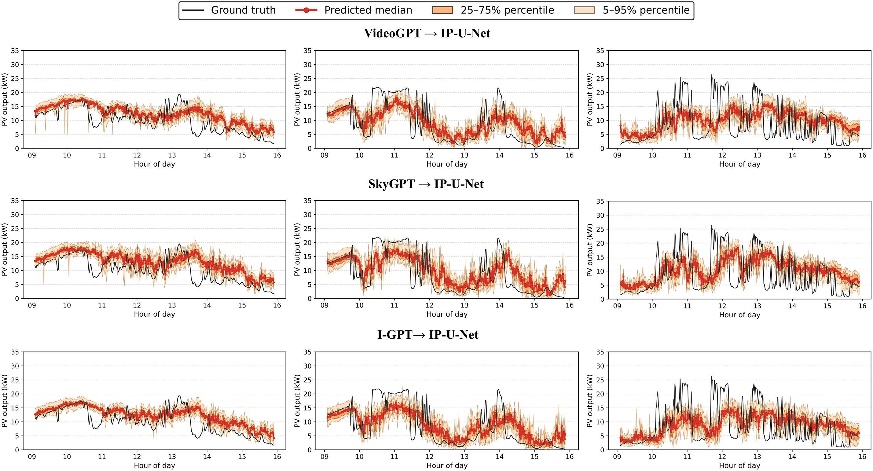
Figure 18: Visualize the prediction curve results of the stochastic prediction model under 3 cloudy conditions in the test set

Generating more future sky images from a random sky image prediction model increases the likelihood of presenting realistic sky image scenarios, but this also increases computational costs. For reference, training the first stage of I-GPT on the entire sky training dataset took nearly 24 h on a single NVIDIA GeForce RTX 4090 GPU. Generating 10 future scenarios for each of the 2582 test set examples required approximately 3.5 h. Therefore, after balancing accuracy gains and runtime, we ultimately selected 10 future scenarios as the configuration parameter for this experiment.

6.2.3 Ablation Experiments for the Proposed PV Output Prediction Model

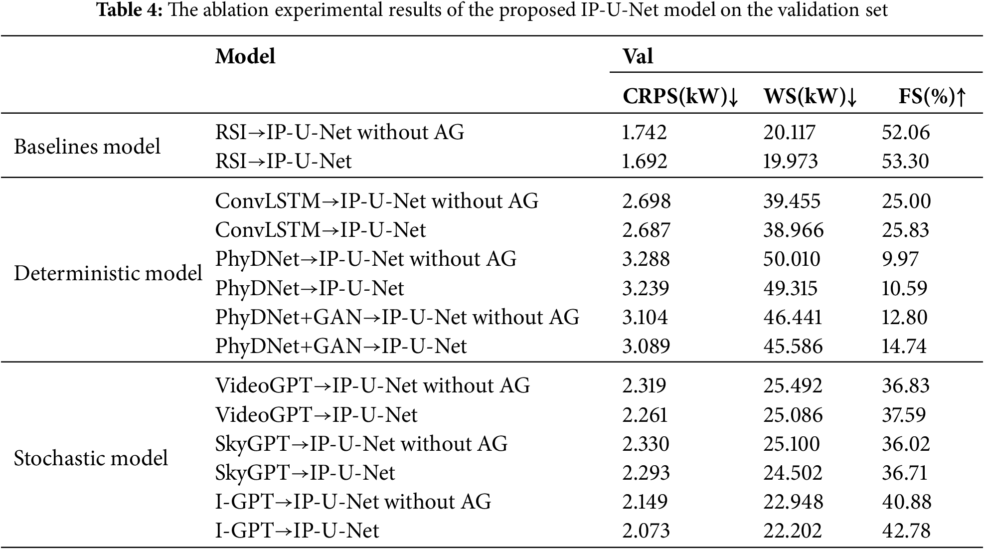
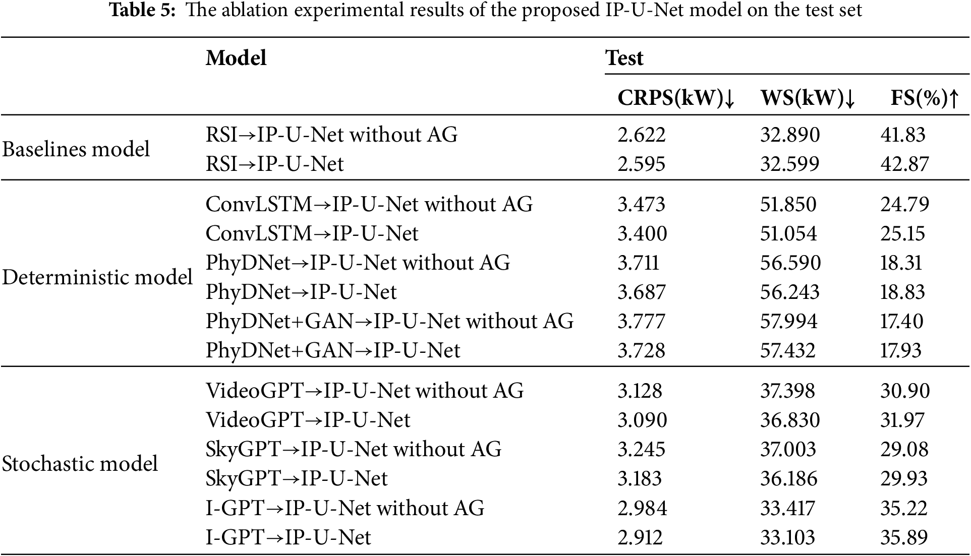
To elucidate the functionality of each component in the proposed IP-U-Net model, this section presents ablation results for different modules on both the validation and test sets, achieved by coupling with sky images generated by the first-stage model. Similarly, all ablation experiments were conducted using cloudy sky samples because sunny sky conditions were excluded during the preprocessing to focus on complex and highly dynamic cloud evolution scenarios. “IP-U-Net without AG” refers to the model with the Attention Gate module removed. The ablation results are shown in Tables 4 and 5. For all three evaluation metrics and across different comparison models, removing the Attention Gate module leads to poorer performance on these metrics, both on the validation and test sets. Notably, it significantly reduces the accuracy of predicting PV probability outputs from the sky images generated in the first stage. This indicates that removing this module weakens the model’s ability to extract effective and critical features from sky images. Particularly for random variations in cloud layers, this severely impacts the precision of predicted probabilities.

6.3 Discussions

We acknowledge several limitations of the present study, which also suggest potential directions for future work. Addressing these issues will further improve the robustness and applicability of the proposed two-stage forecasting framework, particularly for real-world virtual power plant (VPP) operations where prediction reliability and interpretability are both critical.

In this study, we adopted a Transformer-based architecture combined with physics-constrained modules as the backbone for sky image prediction. Although this design achieved satisfactory generative performance and prediction accuracy, a certain gap still remains compared with real future sky images. In recent years, diffusion-based generative models have demonstrated remarkable capabilities in modeling uncertainty and complex dynamics in image and video prediction tasks [50,51]. However, their substantial computational cost and high resource requirements make them difficult to apply in real-time or ultra-short-term photovoltaic power forecasting scenarios. Another consideration is the focus on interpretability under a physics-constrained environment, which further influenced our decision not to include diffusion models in the current experimental comparisons. Nevertheless, we believe that such models hold significant potential for future research. We plan to explore these emerging architectures in subsequent studies to evaluate their advantages in improving prediction sharpness and uncertainty calibration. Furthermore, broader hyperparameter optimization and lightweight architecture exploration will be conducted to balance model performance and inference efficiency, thereby facilitating potential real-time deployment.

The dataset used in this study consists of 53,336 training samples collected from a single location at Stanford University. Although this dataset provides high-quality sky images, its limited geographic scope and climatic homogeneity—particularly the scarcity of cloudy-sky samples—may restrict the model’s generalization under complex meteorological conditions. Transformer-based models such as I-GPT typically benefit from large-scale, diverse datasets. Therefore, future work will focus on expanding the dataset by integrating multi-year, multi-region sky image collections that cover a broader spectrum of weather dynamics. Additionally, transfer learning or few-shot learning techniques could be explored to better leverage heterogeneous datasets and reduce data dependency [52].

Our current framework relies solely on ground-based sky images. Although such imagery effectively captures local cloud evolution, it does not include broader-scale meteorological context. Future research will investigate the integration of additional data modalities—such as satellite observations, numerical weather forecasts, wind velocity, and aerosol concentration—to provide complementary information on cloud advection and atmospheric transparency. The challenge lies in effectively fusing heterogeneous data with different spatial and temporal resolutions. Combining sky images with auxiliary meteorological data is expected to improve both the stability and interpretability of the forecasting process.

7  Conclusion

In summary, this study introduces I-GPT, a stochastic sky image prediction model constrained by multi-scale physical properties. Combined with the IP-U-Net model for predicting PV output from sky images, it forms a two-stage framework for 15-min probabilistic PV forecasting. I-GPT integrates discrete VQ-VAE latent variables with Transformer priors and multi-scale PhyCell-enhanced dynamic features. It fuses physical and appearance paths through a dynamic weight fusion module, generating both realistic and diverse future frames while maintaining consistent cloud advection. When these generated t + 15 sky frames drive IP-U-Net, the end-to-end system achieves an optimal reliability-clarity tradeoff, outperforming deterministic models, other stochastic models, multimodal baseline models, and intelligent persistence models. On the dataset used in our study, it achieves an outstanding CRPS of 2.073 kW and WS of 22.20 kW on the validation set, and CRPS of 2.912 kW and WS of 33.10 kW on the test set. Predictive skill improves by 42.78% and 35.89% over persistence, respectively, and performs exceptionally well on rapidly changing coverage. However, we further observed that while high-quality image generation substantially benefits uncertainty quantification, residual uncertainty is primarily determined by the image-to-PV output mapping. This indicates a need for future research into more robust image-to-PV output prediction models. Additionally, sampling multi-sensor fusion data—such as satellite imagery or multi-camera view images—for training and inference acceleration could be explored to enable large-scale deployment.

Acknowledgement: We would like to express our heartfelt gratitude to all those who have supported and encouraged us throughout the process of completing this thesis. Your guidance and assistance have been invaluable and deeply appreciated.

Funding Statement: This research was supported by the “Regional Innovation Strategy (RIS)” through the National Research Foundation of Korea (NRF) funded by the Ministry of Education (MOE) (2021RIS002) and the Technology Development Program (RS-2025-02312851) funded by the Ministry of SMEs and Startups (MSS, Republic of Korea).

Author Contributions: The authors confirm contribution to the paper as follows: study conception and design: Chen Pan, ChangGyoon Lim; data collection: Chen Pan; analysis and interpretation of results: Chen Pan; draft manuscript preparation: Chen Pan, ChangGyoon Lim. All authors reviewed the results and approved the final version of the manuscript.

Availability of Data and Materials: The data that support the findings of this study are openly available in the Stanford Digital Repository at https://purl.stanford.edu/sm043zf7254 (accessed on 01 November 2025).

Ethics Approval: Not applicable.

Conflicts of Interest: The authors declare no conflicts of interest to report regarding the present study.

Nomenclature

References

1. Wang H, Tang C, Zhao Z, Tang H. Fuzzy logic based admission control for on-grid energy saving in hybrid energy powered cellular networks. KSII Trans Internet Inf Syst. 2016;10(10):4724. doi:10.3837/tiis.2016.10.006. [Google Scholar] [CrossRef]

2. Nie Y, Li X, Paletta Q, Aragon M, Scott A, Brandt A. Open-source sky image datasets for solar forecasting with deep learning: a comprehensive survey. Renew Sustain Energy Rev. 2024;189(3):113977. doi:10.1016/j.rser.2023.113977. [Google Scholar] [CrossRef]

3. Chow CW, Urquhart B, Lave M, Dominguez A, Kleissl J, Shields J, et al. Intra-hour forecasting with a total sky imager at the UC San Diego solar energy testbed. Sol Energy. 2011;85(11):2881–93. doi:10.1016/j.solener.2011.08.025. [Google Scholar] [CrossRef]

4. Blum NB, Nouri B, Wilbert S, Schmidt T, Lünsdorf O, Stührenberg J, et al. Cloud height measurement by a network of all-sky imagers. Atmos Meas Tech. 2021;14(7):5199–224. doi:10.5194/amt-14-5199-2021. [Google Scholar] [CrossRef]

5. Chu Y, Pedro HTC, Coimbra CFM. Hybrid intra-hour DNI forecasts with sky image processing enhanced by stochastic learning. Sol Energy. 2013;98:592–603. doi:10.1016/j.solener.2013.10.020. [Google Scholar] [CrossRef]

6. Chu Y, Li M, Pedro HTC, Coimbra CFM. Real-time prediction intervals for intra-hour DNI forecasts. Renew Energy. 2015;83(6):234–44. doi:10.1016/j.renene.2015.04.022. [Google Scholar] [CrossRef]

7. Paletta Q, Terrén-Serrano G, Nie Y, Li B, Bieker J, Zhang W, et al. Advances in solar forecasting: computer vision with deep learning. Adv Appl Energy. 2023;11(2):100150. doi:10.1016/j.adapen.2023.100150. [Google Scholar] [CrossRef]

8. Sun Y, Venugopal V, Brandt AR. Short-term solar power forecast with deep learning: exploring optimal input and output configuration. Solar Energy. 2019;188:730–41. doi:10.1016/j.solener.2019.06.041. [Google Scholar] [CrossRef]

9. Nie Y, Sun Y, Chen Y, Orsini R, Brandt A. PV power output prediction from sky images using convolutional neural network: the comparison of sky-condition-specific sub-models and an end-to-end model. J Renew Sustain Energy. 2020;12(4):046101. doi:10.1063/5.0014016. [Google Scholar] [CrossRef]

10. Paletta Q, Arbod G, Lasenby J. Benchmarking of deep learning irradiance forecasting models from sky images–An in-depth analysis. Sol Energy. 2021;224(September):855–67. doi:10.1016/j.solener.2021.05.056. [Google Scholar] [CrossRef]

11. Paletta Q, Hu A, Arbod G, Lasenby J. ECLIPSE: envisioning CLoud induced perturbations in solar energy. Appl Energy. 2022;326(6):119924. doi:10.1016/j.apenergy.2022.119924. [Google Scholar] [CrossRef]

12. Zhang L, Wilson R, Sumner M, Wu Y. Advanced multimodal fusion method for very short-term solar irradiance forecasting using sky images and meteorological data: a gate and transformer mechanism approach. Renew Energy. 2023;216(6):118952. doi:10.1016/j.renene.2023.118952. [Google Scholar] [CrossRef]

13. Le Guen V, Thome N. A deep physical model for solar irradiance forecasting with fisheye images. In: 2020 IEEE/CVF Conference on Computer Vision and Pattern Recognition Workshops (CVPRW); 2020 Jun 14–19; Seattle, WA, USA. IEEE; 2020. p. 2685–8. doi:10.1109/cvprw50498.2020.00323. [Google Scholar] [CrossRef]

14. Willert CE, Gharib M. Digital particle image velocimetry. Exp Fluids. 1991;10(4):181–93. doi:10.1007/BF00190388. [Google Scholar] [CrossRef]

15. Huang H, Xu J, Peng Z, Yoo S, Yu D, Huang D, et al. Cloud motion estimation for short term solar irradiation prediction. In: 2013 IEEE International Conference on Smart Grid Communications (SmartGridComm); 2013 Oct 21–24; Vancouver, BC, Canada: IEEE; 2013. p. 696–701. doi:10.1109/SmartGridComm.2013.6688040. [Google Scholar] [CrossRef]

16. Dev S, Savoy FM, Lee YH, Winkler S. Short-term prediction of localized cloud motion using ground-based sky imagers. In: 2016 IEEE Region 10 Conference (TENCON); 2016 Nov 22–25; Singapore. p. 2563–6. doi:10.1109/TENCON.2016.7848499. [Google Scholar] [CrossRef]

17. Zelikman E, Zhou S, Irvin J, Raterink C, Sheng H, Avati A, et al. Short-term solar irradiance forecasting using calibrated probabilistic models. arXiv:201004715. 2020. doi:10.48550/arXiv.2010.04715. [Google Scholar] [CrossRef]

18. Wan C, Xu Z, Pinson P, Dong ZY, Wong KP. Probabilistic forecasting of wind power generation using extreme learning machine. IEEE Trans Power Syst. 2014;29(3):1033–44. doi:10.1109/TPWRS.2013.2287871. [Google Scholar] [CrossRef]

19. Wang Y, Gan D, Sun M, Zhang N, Lu Z, Kang C. Probabilistic individual load forecasting using pinball loss guided LSTM. Appl Energy. 2019;235:10–20. doi:10.1016/j.apenergy.2018.10.078. [Google Scholar] [CrossRef]

20. Paletta Q, Arbod G, Lasenby J. Omnivision forecasting: combining satellite and sky images for improved deterministic and probabilistic intra-hour solar energy predictions. Appl Energy. 2023;336(6):120818. doi:10.1016/j.apenergy.2023.120818. [Google Scholar] [CrossRef]

21. Hu A, Cotter F, Mohan N, Gurau C, Kendall A. Probabilistic future prediction for video scene understanding. In: Computer vision—ECCV 2020. Cham, Switzerland: Springer International Publishing; 2020. p. 767–85. doi:10.1007/978-3-030-58517-4_45. [Google Scholar] [CrossRef]

22. Ravuri S, Lenc K, Willson M, Kangin D, Lam R, Mirowski P, et al. Skilful precipitation nowcasting using deep generative models of radar. Nature. 2021;597(7878):672–7. doi:10.1038/s41586-021-03854-z. [Google Scholar] [PubMed] [CrossRef]

23. Cheng J, Yang Y, Tang X, Xiong N, Zhang Y, Lei F. Generative adversarial networks: a literature review. KSII Trans Internet Inf Syst. 2023;14:4625–47. doi:10.3837/tiis.2020.12.001. [Google Scholar] [CrossRef]

24. Vaswani A, Shazeer N, Parmar N, Uszkoreit J, Jones L, Gomez AN, et al. Attention is all you need. Adv Neural Inf Process Syst. 2017;30:1–11. doi:10.48550/arXiv.1706.03762. [Google Scholar] [CrossRef]

25. Shi X, Chen Z, Wang H, Yeung DY, Wong WK, Woo WC. Convolutional LSTM network: a machine learning approach for precipitation nowcasting. Adv Neural Inf Process Syst. 2015;28:1–9. [Google Scholar]

26. Wang Y, Zhang J, Zhu H, Long M, Wang J, Yu PS. Memory in memory: a predictive neural network for learning higher-order non-stationarity from spatiotemporal dynamics. In: 2019 IEEE/CVF Conference on Computer Vision and Pattern Recognition (CVPR); 2019 Jun 15–20; Long Beach, CA, USA. IEEE; 2019. p. 9146–54. doi:10.1109/CVPR.2019.00937. [Google Scholar] [CrossRef]

27. Guen VL, Thome N, editors. Disentangling physical dynamics from unknown factors for unsupervised video prediction. In: Proceedings of the IEEE/CVF Conference on Computer Vision and Pattern Recognition; 2020 Jun 13–18; Seattle, WA, USA. p. 13–9. doi:10.48550/arXiv.2003.01460. [Google Scholar] [CrossRef]

28. Kingma DP, Welling M. Auto-encoding variational bayes. arXiv:13126114. 2013. doi:10.48550/arXiv.1312.6114. [Google Scholar] [CrossRef]

29. Goodfellow IJ, Pouget-Abadie J, Mirza M, Xu B, Warde-Farley D, Ozair S, et al. Generative adversarial nets. Adv Neural Inf Process Syst. 2014;27(11):1–9. doi:10.1145/3422622. [Google Scholar] [CrossRef]

30. Lee AX, Zhang R, Ebert F, Abbeel P, Finn C, Levine S. Stochastic adversarial video prediction. arXiv:180401523. 2018. Available from: http://arxiv.org/abs/1804.01523. [Google Scholar]

31. Yan W, Zhang Y, Abbeel P, Srinivas A. Videogpt: video generation using vq-vae and transformers. arXiv:210410157. 2021. Available from: http://arxiv.org/abs/2104.10157. [Google Scholar]

32. Nie Y, Zelikman E, Scott A, Paletta Q, Brandt A. SkyGPT: probabilistic ultra-short-term solar forecasting using synthetic sky images from physics-constrained VideoGPT. Adv Appl Energy. 2024;14(11):100172. doi:10.1016/j.adapen.2024.100172. [Google Scholar] [CrossRef]

33. Andrianakos G, Tsourounis D, Oikonomou S, Kastaniotis D, Economou G, Kazantzidis A. Sky image forecasting with generative adversarial networks for cloud coverage prediction. In: 2019 10th International Conference on Information, Intelligence, Systems and Applications (IISA); 2019 Jul 15–17; Patras, Greece. IEEE; 2019. p. 1–7. doi:10.1109/IISA.2019.8900774. [Google Scholar] [CrossRef]

34. Meddahi A, Tuomiranta A, Guillon S. Skill-driven data sampling and deep learning framework for minute-scale solar forecasting with sky images. Sol RRL. 2025;9(4):2400664. doi:10.1002/solr.202400664. [Google Scholar] [CrossRef]

35. Liu CL, Lu SR, Chen YT, Lee CH. Temporal attention for photovoltaic power forecasting using all-sky imagery. Sustain Energy Grids Netw. 2025;44(3):101985. doi:10.1016/j.segan.2025.101985. [Google Scholar] [CrossRef]

36. Alvares CA, Stape JL, Sentelhas PC, De Moraes Gonçalves JL, Sparovek G. Köppen’s climate classification map for Brazil. Meteorol Z. 2014;22(6):711–28. doi:10.1127/0941-2948/2013/0507. [Google Scholar] [CrossRef]

37. Nie Y, Li X, Scott A, Sun Y, Venugopal V, Brandt A. SKIPP’D: a SKy images and photovoltaic power generation dataset for short-term solar forecasting. Sol Energy. 2023;255(10):171–9. doi:10.1016/j.solener.2023.03.043. [Google Scholar] [CrossRef]

38. Van Den Oord A, Vinyals O. Neural discrete representation learning. Adv Neural Inf Process Syst. 2017;30:1–10. [Google Scholar]

39. Chen M, Radford A, Child R, Wu J, Jun H, et al. editors. Generative pretraining from pixels. In: Proceedings of the International Conference on Machine Learning; 2020 Jul 13–18; Virtual. p. 1691–703. Available from: https://proceedings.mlr.press/v119/chen20s/chen20s.pdf. [Google Scholar]

40. Ba JL, Kiros JR, Hinton GE. Layer normalization. arXiv:160706450. 2016. doi:10.48550/arXiv.1607.06450. [Google Scholar] [CrossRef]

41. Huang Z, Wang X, Huang L, Huang C, Wei Y, Liu W. Ccnet: criss-cross attention for semantic segmentation. In: Proceedings of the IEEE/CVF International Conference on Computer Vision; 2019 Oct 27–Nov 2; Seoul, Republic of Korea. p. 603–12. doi:10.48550/arXiv.1811.11721. [Google Scholar] [CrossRef]

42. Ho J, Kalchbrenner N, Weissenborn D, Salimans T. Axial attention in multidimensional transformers. arXiv:191212180. 2019. doi:10.48550/arXiv.1912.12180. [Google Scholar] [CrossRef]

43. Ronneberger O, Fischer P, Brox T editors. U-net: convolutional networks for biomedical image segmentation. In: Proceedings of the International Conference on Medical Image Computing and Computer-assisted Intervention; 2015 Oct 5–9; Munich, Germany. p. 234–41. doi:10.48550/arXiv.1505.04597. [Google Scholar] [CrossRef]

44. Simonyan K, Zisserman A. Very deep convolutional networks for large-scale image recognition. arXiv:14091556. 2014. doi:10.48550/arXiv.1409.1556. [Google Scholar] [CrossRef]

45. Gneiting T, Katzfuss M. Probabilistic forecasting. Annu Rev Stat Appl. 2014;1(1):125–51. doi:10.1146/annurev-statistics-062713-085831. [Google Scholar] [CrossRef]

46. Winkler RL. A decision-theoretic approach to interval estimation. J Am Stat Assoc. 1972;67(337):187–91. doi:10.1080/01621459.1972.10481224. [Google Scholar] [CrossRef]

47. Da Rosa AV, Ordonez JC. Fundamentals of renewable energy processes. Cambridge, MA, USA: Academic Press; 2021. doi:10.1016/B978-0-12-374639-9.X0001-2. [Google Scholar] [CrossRef]

48. Kingma DP. Adam: a method for stochastic optimization. arXiv:14126980. 2014. doi:10.48550/arXiv.1412.6980. [Google Scholar] [CrossRef]

49. Pan C, Liu Y, Oh Y, Lim C. Short-term photovoltaic power forecasting using PV data and sky images in an auto cross modal correlation attention multimodal framework. Energies. 2024;17(24):6378. doi:10.3390/en17246378. [Google Scholar] [CrossRef]

50. Zhang Z, Hu J, Cheng W, Paudel D, Yang J. Extdm: distribution extrapolation diffusion model for video prediction. In: Proceedings of the IEEE/CVF Conference on Computer Vision and Pattern Recognition; 2024 Jun 16–22; Seattle, WA, USA. p. 19310–20. [Google Scholar]

51. Wang Y, Liu X, Pang W, Ma L, Yuan S, Debevec P, et al. Survey of video diffusion models: foundations, implementations, and applications. arXiv:250416081. 2025. doi:10.48550/arXiv.2504.16081. [Google Scholar] [CrossRef]

52. Paletta Q, Nie Y, Saint-Drenan YM, Le Saux B. Improving cross-site generalisability of vision-based solar forecasting models with physics-informed transfer learning. Energy Convers Manag. 2024;309(2):118398. doi:10.1016/j.enconman.2024.118398. [Google Scholar] [CrossRef]