
 Submit a Paper
 Propose a Special lssue
 Open Access
ARTICLE

Attention-Enhanced ResNet-LSTM Model with Wind-Regime Clustering for Wind Speed Forecasting
1 Department of Bridge Engineering, Southwest Jiaotong University, Chengdu, 610031, China
2China Railway Construction Bridge Bureau Group Corporation, Wuhan, 430034, China
3 State Key Laboratory of Bridge Intelligent and Green Construction, Wuhan, 430034, China
* Corresponding Author: Enbo Yu. Email:
Computer Modeling in Engineering & Sciences 2026, 146(1), 25 https://doi.org/10.32604/cmes.2025.069733
Received 29 June 2025; Accepted 01 September 2025; Issue published 29 January 2026
 View Full Text
 Download PDF
Abstract
Accurate wind speed prediction is crucial for stabilizing power grids with high wind energy penetration. This study presents a novel machine learning model that integrates clustering, deep learning, and transfer learning to mitigate accuracy degradation in 24-h forecasting. Initially, an optimized DB-SCAN (Density-Based Spatial Clustering of Applications with Noise) algorithm clusters wind fields based on wind direction, probability density, and spectral features, enhancing physical interpretability and reducing training complexity. Subsequently, a ResNet (Residual Network) extracts multi-scale patterns from decomposed wind signals, while transfer learning adapts the backbone network across clusters, cutting training time by over 90%. Finally, a CBAM (Convolutional Block Attention Module) attention mechanism is employed to prioritize features for LSTM-based prediction. Tested on the 2015 Jena wind speed dataset, the model demonstrates superior accuracy and robustness compared to state-of-the-art baselines. Key innovations include: (a) Physics-informed clustering for interpretable wind regime classification; (b) Transfer learning with deep feature extraction, preserving accuracy while minimizing training time; and (c) On the 2016 Jena wind speed dataset, the model achieves MAPE (Mean Absolute Percentage Error) values of 16.82% and 18.02% for the Weibull-shaped and Gaussian-shaped wind speed clusters, respectively, demonstrating the model’s robust generalization capacity. This framework offers an efficient and effective solution for long-term wind forecasting.Keywords
In the 21st century, wind power has gained significant attention as a sustainable alternative to traditional fossil energy sources. The global installed capacity for wind power has rapidly increased in recent years, and this trend is expected to persist, driven by advancements in technology and increased environmental concerns [1–3]. As wind power generation is highly dependent on the wind environment surrounding the base station, it is crucial to manage the uncertainty of wind speed conditions in the short term to rationalize power supply schedules and maintain the stability and efficiency of power transmission networks [4].
Recent advancements in data-driven approaches for wind speed prediction, particularly the development of neural network models, have proven to be reliable in simulating the near-surface wind field. Unlike traditional modeling techniques that rely on collecting local weather data (e.g., humidity, atmospheric pressure, etc.) to find a physical solution, neural network models offer advantages in terms of input data quantity, model complexity, and computational efficiency [5,6].
In-depth studies have demonstrated various data processing methods and surrogate models for ultra-short-time wind speed predictions, including Kalman filters [7,8], Gaussian processes [9], firefly algorithm [10], fuzzy system [11,12], XGBoost model [13] and so on. Among these, the CEEMDAN (Complete Ensemble Empirical Mode Decomposition with Adaptive Noise) algorithm, introduced in 2011, has attracted considerable attention in recent years due to its exceptional convergence properties [14,15]. The CEEMDAN method has been successfully applied in fields such as physics, chemistry, economics, and biophysics, and has gradually found its place in wind speed prediction [16,17].
However, although the CEEMDAN approach enhances the predictability of wind environments, current models predominantly focus on ultra-short-term wind forecasts with time spans of less than one hour. As the forecast horizon extends, the generalization ability of these models becomes limited due to the highly nonlinear nature of the wind field and the reduced autocorrelation of time series data. This results in suboptimal predictions for longer-term forecasts [18]. Several studies have demonstrated that prediction accuracy decreases significantly as the forecasting horizon increases from one hour to 24 h [19,20]. This indicates that existing models struggle to provide high-accuracy predictions over extended time periods, limiting their applicability in real-world engineering projects.
The challenges with these models stem from several factors. First, mainstream feature extraction techniques in wind prediction models largely rely on shallow neural networks. For example, He et al. [21] employed a deep belief network (DBN) with three hidden layers, while Han et al. [22] used a convolutional neural network (CNN) with two hidden layers. Research suggests that deep neural networks are more effective than shallow ones at extracting features from complex data. Thus, there is a need for deeper and more efficient feature extraction networks. Second, wind direction is an important factor in determining wind speed variations, both from a meteorological and geographical perspective. However, many studies have only considered the correlation between wind direction and wind speed, without exploring the physical mechanisms underlying this relationship to enhance prediction accuracy. Finally, the contribution of extracted features to prediction accuracy varies, making it essential to incorporate attention mechanisms (AM) that assign appropriate weights to different features to improve model performance.
Recent work on Transformer-based models has demonstrated their potential in time series forecasting, including wind speed prediction. Transformers are well-suited for capturing long-range dependencies within sequential data due to their self-attention mechanism, which allows the model to focus on relevant data points without being constrained by fixed window sizes [23]. However, despite these strengths, Transformer models face limitations in wind speed prediction. The computational cost of training and deploying large Transformer models can be prohibitively high for high-frequency wind measurements and low-power edge hardware [24]. Transformers may also struggle with non-stationarity and volatility in wind speed data, which often exhibits sudden changes that require extensive pre-processing [25]. While Transformers excel at long-range dependencies, they can lack the interpretability needed in meteorology. For edge deployment and real-time wind forecasting, lightweight hybrid architectures such as CNN-LSTM offer a favorable trade-off: CNN layers extract local spatial/temporal features efficiently and LSTM units model short-to-medium dynamics with far fewer parameters and lower inference latency than common Transformer variants, yielding superior practical performance on resource-constrained devices in recent studies [26,27]. This study therefore adopts a lightweight design incorporating spatial and channel attention mechanisms into the model architecture, aiming to preserve interpretability for physical analysis and reduce latency.
Building on these advancements, this paper proposes a novel wind speed prediction model that integrates wind field classification with efficient feature extraction techniques for 24-h forecasting. The model comprises three sub-modules: classification, feature extraction, and prediction. First, the wind field dataset is classified using an optimized DB-SCAN (Density-Based Spatial Clustering of Applications with Noise) algorithm based on physical parameters. Next, a deep ResNet (Residual Network) with a feature pyramid framework is employed for scalable feature extraction, incorporating depth-wise convolution kernels and transfer learning to reduce computational cost. Finally, the extracted features are weighted through a CBAM (Convolutional Block Attention Module) and passed into an LSTM (Long Short-Term Memory) layer for prediction.
The novelty of this study lies in three key innovations: (1) the development of an interpretable prediction model grounded in wind field characteristics, using wind direction as a label and integrating wind speed probability density distributions and energy spectra as clustering criteria; (2) the deployment of a ResNet-18 network with feature fusion to demonstrate the effectiveness of deep neural networks in wind speed feature extraction; and (3) the application of transfer learning to construct dedicated backbone networks for each wind speed cluster, enhancing computational efficiency while maintaining prediction accuracy.
The remainder of the paper is organized as follows. Section 2 introduces the dataset used for model training. Section 3 details the architecture and methodology of the proposed model, while Section 4 describes the operating environment and loss function. Section 5 verifies the reliability and validity of the proposed model through controlled comparative experiments. Section 6 illustrates the model’s applicability using rolling forecasts on a new dataset. Finally, Section 7 presents concluding remarks.
Germany, situated in central Europe within the westerly zone between the continental climates of the eastern Atlantic, is a pioneer in wind energy utilization and hosts the largest onshore wind power market in Europe [28]. In this study, the 2015 wind speed dataset from the city of Jena in Thuringia is employed, with its geographical location shown in Fig. 1. The dataset, recorded by the Max-Planck-Gesellschaft weather station, comprises 52,560 ten-minute average wind speed observations for the year.
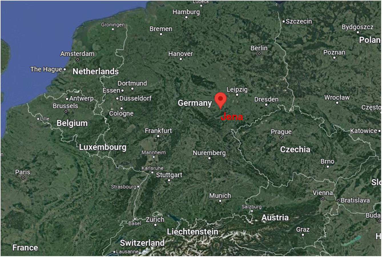
Figure 1: The geography of Jena city
By dividing the spatial direction into 16 equal parts, the distribution of the wind direction in the Jena region throughout the year is counted and displayed in Fig. 2. In the figure, the intersection of the red line with each direction represents the frequency of wind direction occurrence
where
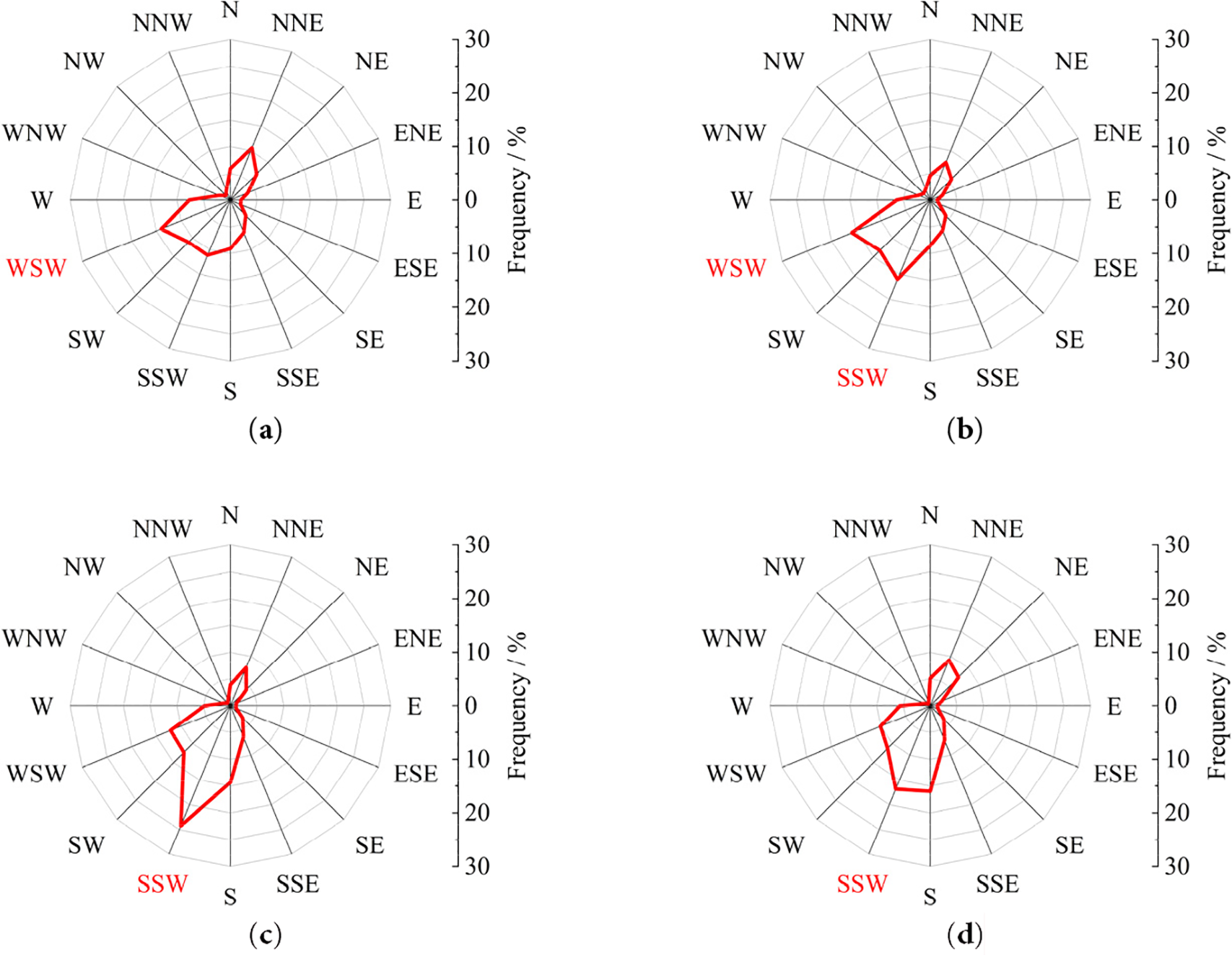
Figure 2: Wind direction frequency distribution of Jena. (a) Frequency distribution map of winter wind direction, (b) Frequency distribution map of spring wind direction, (c) Frequency distribution map of autumn wind direction, (d) Frequency distribution map of summer wind direction
As can be noted in Fig. 2, southwest winds dominate during winter, while rising temperatures gradually shift the prevailing direction toward the northeast, reflecting the seasonal transformation of regional wind patterns. This indicates that wind direction in Jena evolves continuously over time; therefore, the prevailing wind direction during each period is adopted as the primary reference for this study.
Section 3 details the methodology developed for multi-step wind speed prediction, centered on a hybrid model integrating optimized clustering, signal decomposition, and deep learning. The overall process, depicted in Fig. 3, begins with comprehensive data preprocessing and statistical analysis of the wind field characteristics. This is followed by an optimized density-based clustering algorithm applied to categorize wind regimes based on distribution shape and spectral properties, significantly reducing computational complexity and filtering unrepresentative data. Subsequently, the CEEMDAN method decomposes the clustered wind speed time series into IMFs (intrinsic mode functions) to facilitate feature extraction. A specialized backbone network, based on ResNet-18 architecture enhanced with multi-scale fusion and attention mechanisms, then processes these IMFs. Finally, transfer learning techniques are employed to efficiently adapt the feature extraction capabilities across different identified clusters.
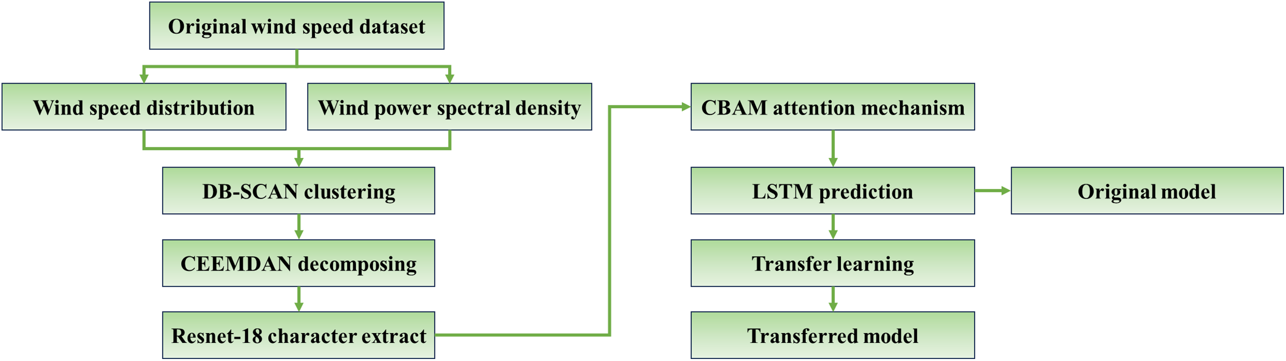
Figure 3: Overall process flow diagram of the proposed model
This structured approach, as depicted in the workflow in Fig. 3, facilitates robust feature learning and the training of prediction models that are specifically tailored to local wind field dynamics, beginning with a foundational analysis of the underlying wind characteristics. A detailed description of the model components will be provided in the latter section of Section 3.
In the realm of wind field studies, wind characteristics typically encompass parameters such as mean wind speed, turbulence intensity, wind speed distribution, power density spectrum, and other related factors. Within these parameters, the frequency distribution of wind speed is often determined by assessing the occurrences of different wind speeds in observations and fitting the probabilities with functional equations. In wind engineering research, the two commonly employed fitting equations include the Gaussian fit [29] and the two-parameter Weibull fit [30], and the probability distribution functions for these two fits are presented in Eqs. (2) and (3), respectively.
where in Eq. (2),
Fig. 4a,b illustrates the minimum residual fit for two distinct wind speed conditions, where the wind speed data are derived by extracting time series with a length of 10 days (1440 timesteps) from the database. Examining the fitting curve in Fig. 4, it is noteworthy that the Weibull probability density distribution is more fitting for low wind speed time series, while those trending towards a Gaussian distribution exhibit the opposite behavior. The assessment of the more suitable curve for fitting the probability density distribution of a wind speed sequence can be made by analyzing residual values.
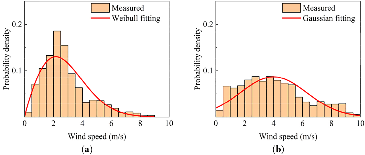
Figure 4: Wind speed probability density distributions and fitting functions: (a) Weibull distribution; (b) Gaussian distribution
The PSD (power spectral density) function can demonstrate the energy distribution of the wind field in different frequency bands through a time-frequency domain transformation. Since the CEEMDAN algorithm can conduct a decomposition of the frequency components, an analysis for the contribution magnitude of each frequency component is necessary for prediction, and this part is discussed in detail in Section 3.3. In the Jena city, the difference of wind PSD functions is pronounced for varying incoming directions. Taking the wind field in southwest and northeast directions as examples, 500 random selected sets for the wind speed data with 10-day length from each direction are taken for PSD calculation, and the averaged polynomial fitting results are presented in Fig. 5a,b, respectively. In Fig. 5, the ordinate is set as
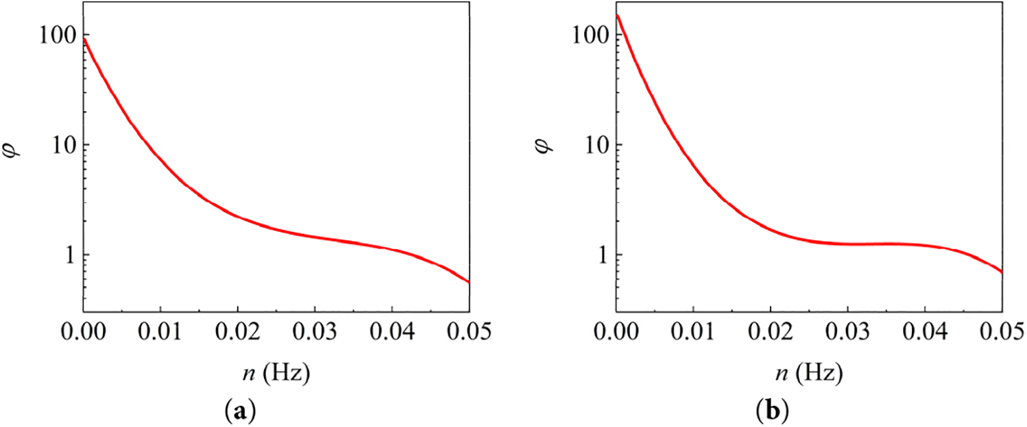
Figure 5: PSD fitting polyline for wind fields with different incoming directions: (a) Southwest; (b) Northeast
The statistics presented in Fig. 5 indicate that the wind fields exhibit variously in energy distribution across different wind directions. Compared with the northeast wind field, the energy carried by the southwest wind is higher in the low frequency region and decays much more slowly as the frequency progressively increases. Hence, from a spectral perspective, the southwestern wind carries stronger energy, which indicates that the Jena city is exposed to more vigorous wind conditions during the winter months. This statistical analysis reinforces the desirability of establishing a hybrid model to reduce the generalization difficulty.
3.2 Optimized DB-SCAN Clustering Model
Long-term empirical studies have confirmed that the wind speed distribution and spectral characteristics of wind fields vary with wind direction for the same measurement area [31,32]. Moreover, the analysis in Section 3.1 demonstrates that this observation also applies to the wind field in Jena, which makes it possible to establish a cluster model for local wind fields. On the one hand, wind fields with comparable characteristics can be filtered by cluster analysis, and on the other hand, unrepresentative data sequences can be excluded, thus reducing the risk of overfitting and speeding up training.
The adaptive nature of model classification is emphasized in the process of clustering model establishment. Due to the randomness and complexity of the wind field variability, certain hyperparameters commonly required in clustering models, including clustering initialization conditions, number of classifications, etc., are costly to optimize through parameter tuning. In addition, as the wind field clustering does not follow a spherical distribution, the selected algorithm is expected to perform well for arbitrarily shaped distributions. Finally, as the unrepresentative time series from the dataset are supposed to be removed during the cluster process, an algorithm insensitive to noise is preferred.
DB-SCAN is a density-based clustering method, which favorably meets the requirements presented above. The DB-SCAN model performs clustering by neighborhood-parameter
The main steps of the DB-SCAN algorithm are demonstrated as follows.
(1) Set the minimum threshold value for
(2) Find all components that are at a distance less than
(3) Allocate each non-core point to a nearby cluster if the cluster is subordinate to
Fig. 6 demonstrates the cluster situation with a
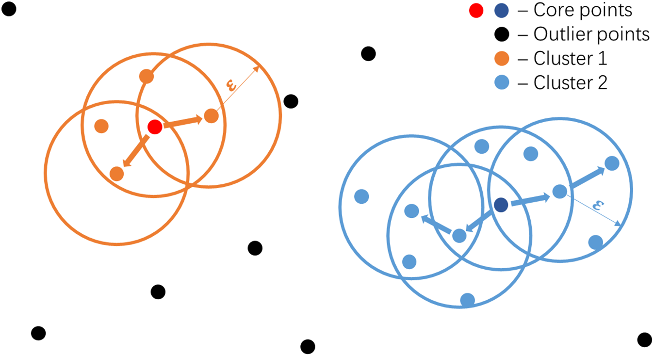
Figure 6: Schematic diagram for DB-SCAN model clustering process
However, the DB-SCAN algorithm still has a drawback in case applications, as the database contains more than 500,000 time series. Given the quadratic relationship between the computational complexity of the DB-SCAN sub-model and the volume of data, enhancing computational efficiency becomes a crucial endeavor. To address this problem, a three-step optimized DB-SCAN clustering sub-model is proposed and demonstrated as Fig. 7.
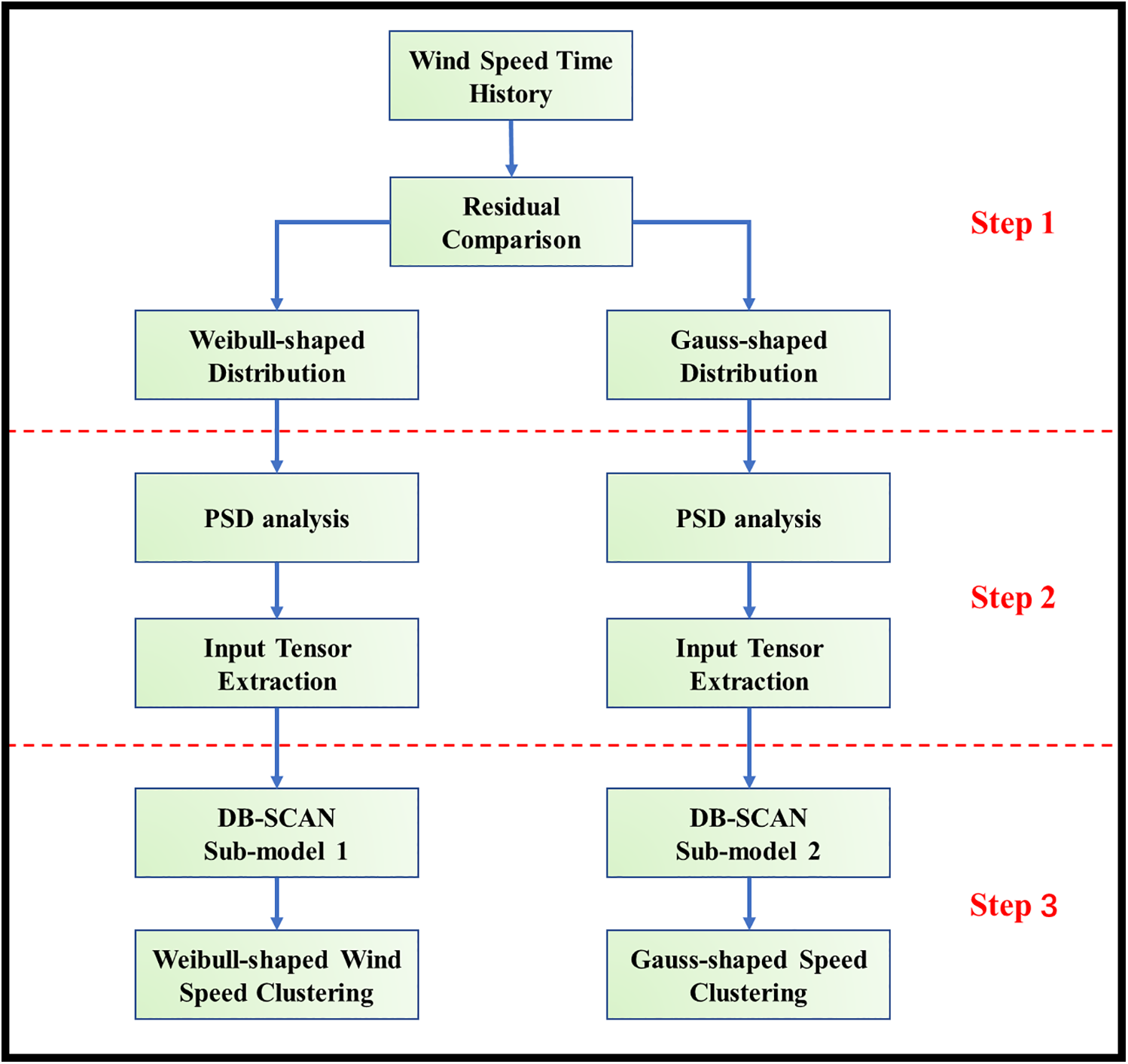
Figure 7: Optimized clustering algorithm flowchart
In step 1, the wind speed time series are categorized into two distinct groups, characterized by either Weibull-shaped or Gaussian-shaped distributions. This categorization is accomplished through a comparison of the fitting residuals.
In the subsequent step 2, the wind speed data undergo a transformation into PSD functions with spectral analysis methods. This transformation enables the extraction of energy distribution across various frequencies within the wind field, resulting in the generation of a feature tensor. To illustrate the processes in step 2, the analysis process on Weibull-shaped wind field is taken as an example, as demonstrated in Fig. 8.
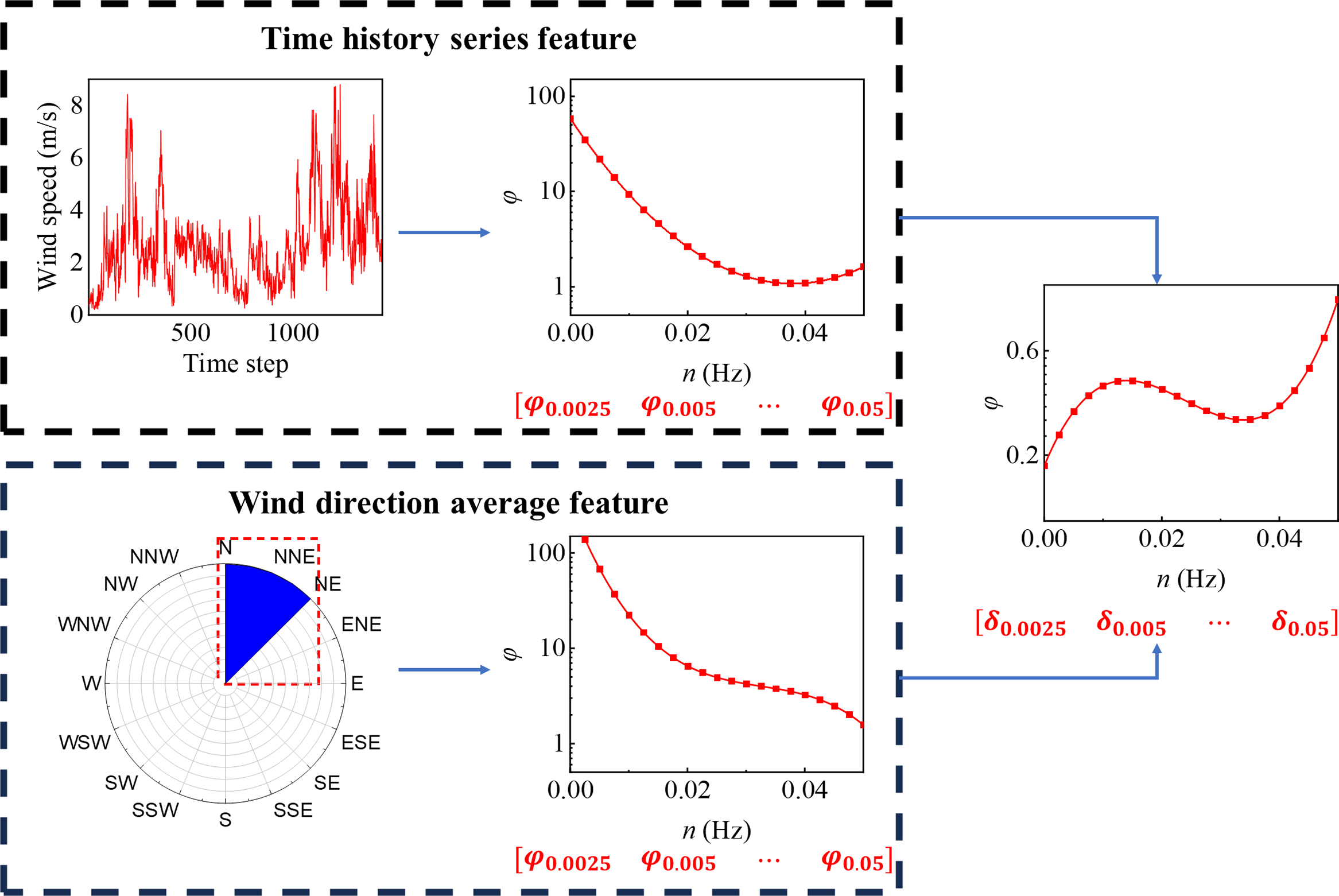
Figure 8: The analysis process of feature tensor in step 2
As illustrated in Fig. 8, with the spectral analysis of the wind speed time series, the spectrum function in the range of 0 to 5 Hz can be derived. By sampling this spectrum function at intervals of 0.0025 Hz, a spectrum feature tensor
In step 3, the feature tensor
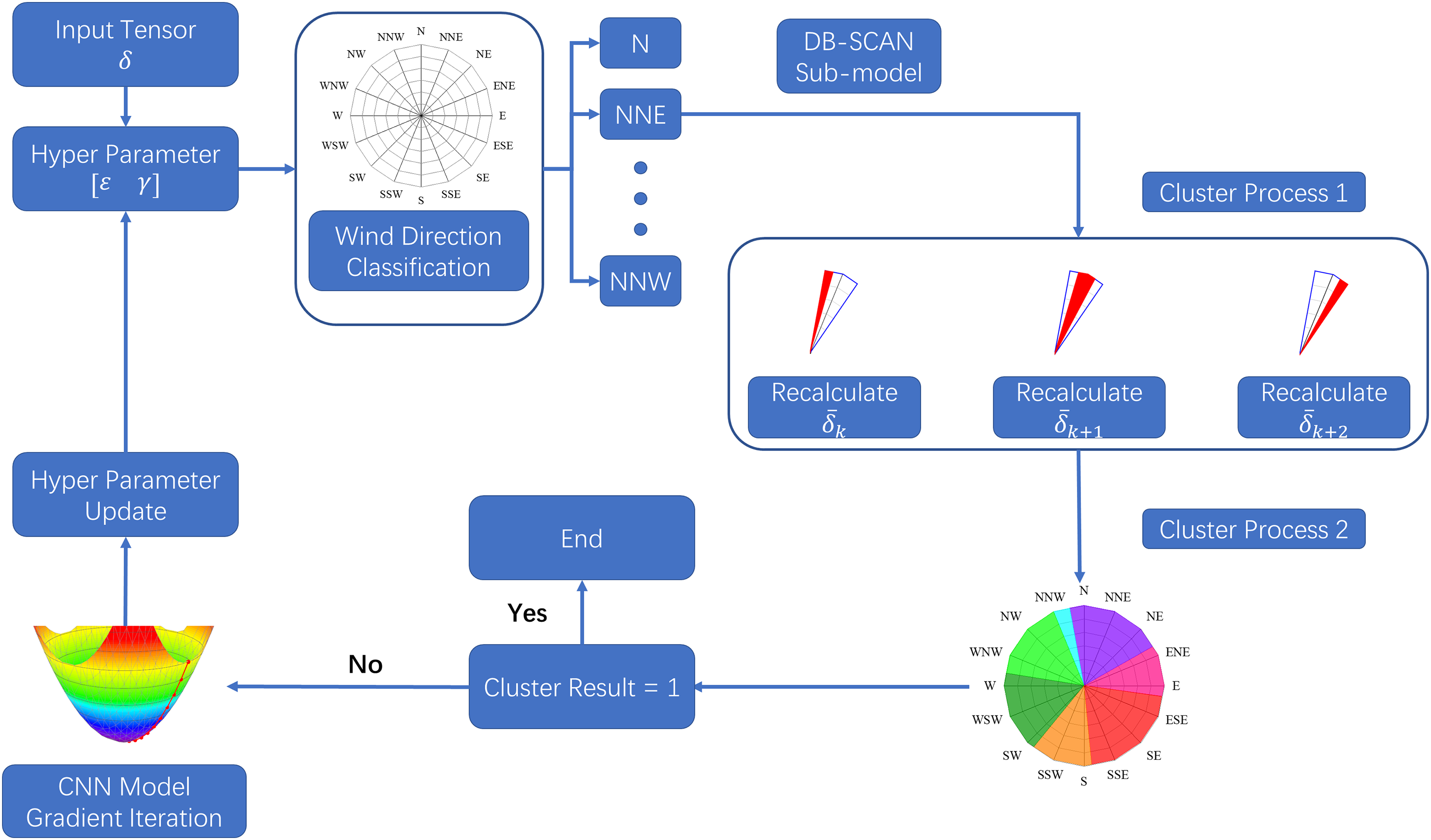
Figure 9: Process flow diagram for step 3
According to Fig. 9, two clustering phases are conducted using the DB-SCAN algorithm within the execution. Initially, hyperparameters are set with
Through the step 2 and step 3, the Weibull-shaped and Gaussian-shaped wind speed time series can be clustered by DB-SCAN algorithm. In the operation of the optimized DB-SCAN sub-model, the computations are simplified, and this simplification can be described using Kolmogorov complexity. This complexity measures the shortest program length needed to generate the final clustering results, and can be manifested in the following aspects:
• The wind speed time series data (1 × 1440 tensor) is characterized by its high dimensionality and the challenge of conducting inter-data comparisons. However, employing a spectral analysis approach allows for the transformation of this time series data into a low-dimensional tensor δ (1 × 20 tensor) that represents the energy distribution. This effectively reduces the number of variables in the input tensor for the DB-SCAN sub-model.
• Informed by the physical insight that wind speed data from the same wind direction exhibit spectral similarity, a two-step clustering approach using the DB-SCAN algorithm is implemented to mitigate computational complexity. The degree of efficiency in this reduction of computational complexity is contingent upon the distribution of wind speed data. For 16 wind directions, if the number of wind speed sequences included in each wind direction ranges from
• The DB-SCAN model categorizes wind speed data with akin characteristics into the same cluster while excluding non-representative wind speed data. Consequently, this procedure significantly diminishes the training complexity of the prediction sub-model when appropriate clustering is executed, as further substantiated by the experiments detailed in Section 5.
The number of clusters within last 25 loops from step 3 are displayed in Fig. 10a,b.
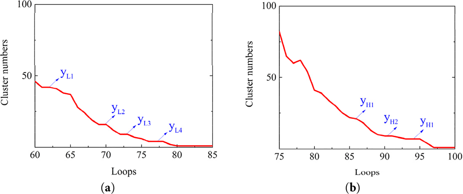
Figure 10: DB-SCAN sub-model iteration outcomes: (a) sub-model 1 (low wind speed cluster); (b) sub-model 2 (high wind speed cluster)
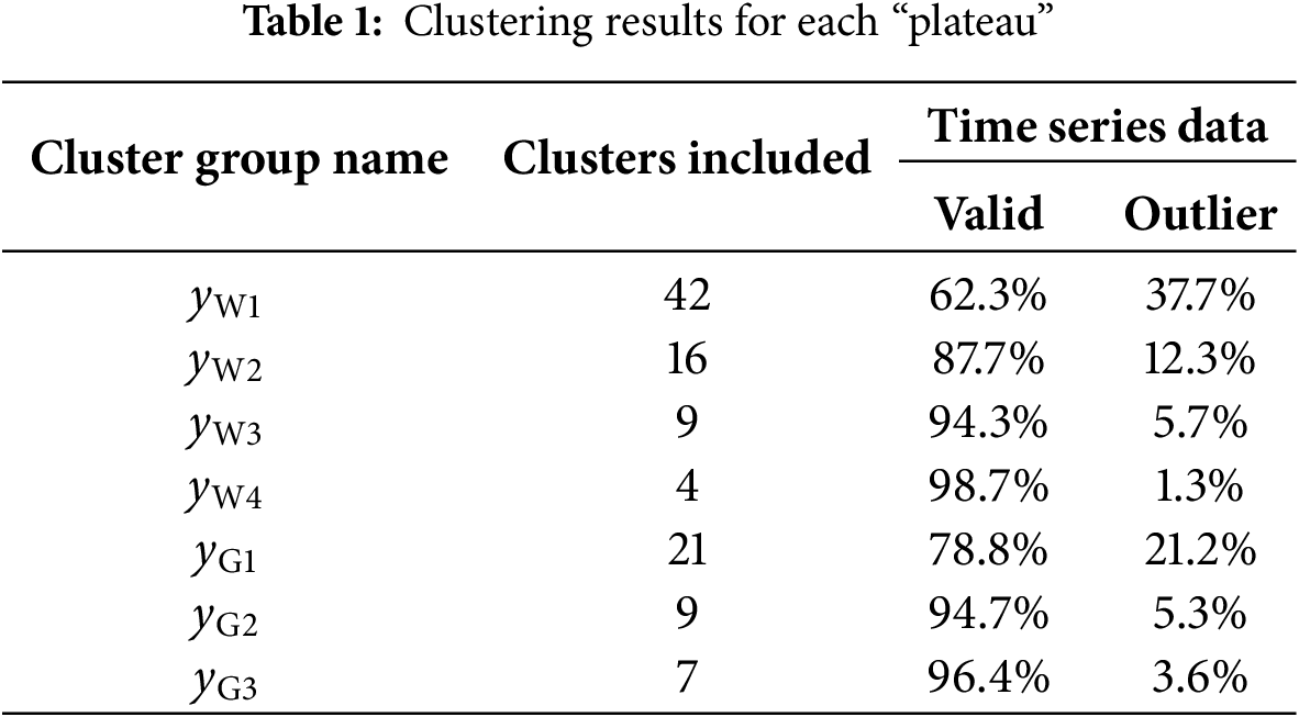
From Fig. 10, it can be concluded that during the operation of model tunning, there are “plateau” phenomena, i.e., as the iteration number increases, the clustering results remain invariant. This observation indicates that the clustering has reached a relatively stationary status. Therefore, the plateaus of the polyline in Fig. 10a,b suggest reasonable clustering results for wind speed time series. In the last 25 iterations, the cluster numbers corresponding to the “plateau” of Weibull-shaped wind series and Gaussian-shaped wind series are designated as
The CEEMDAN method is a derivative of the EMD method, which employs the Gaussian white noise to the decomposition process to suppress modal aliasing. The signal to be decomposed is illustrated as Eq. (6).
where
Subsequently,
where
Therefore, the relationship between the original signal and the decomposed IMFs is satisfied as illustrated in Eq. (9).
The CEEMDAN algorithm enables the original signal to be decomposed into a number of partially orthogonal IMF bands, thus reducing the learning difficulty of the neural network model.
Taking the average wind speed data recorded from 01 January to 10 January in 2015 as an example, the original signal and the corresponding nine decomposed IMF bands are illustrated in Fig. 11. In the figure, for each sub-plot, the horizontal coordinate represents a total of 1440 timesteps for the studied time series wind speed, where each timestep refers to a duration of 10 min. The vertical coordinate denotes to the wind speed corresponding to each IMF signal with the unit of m/s.
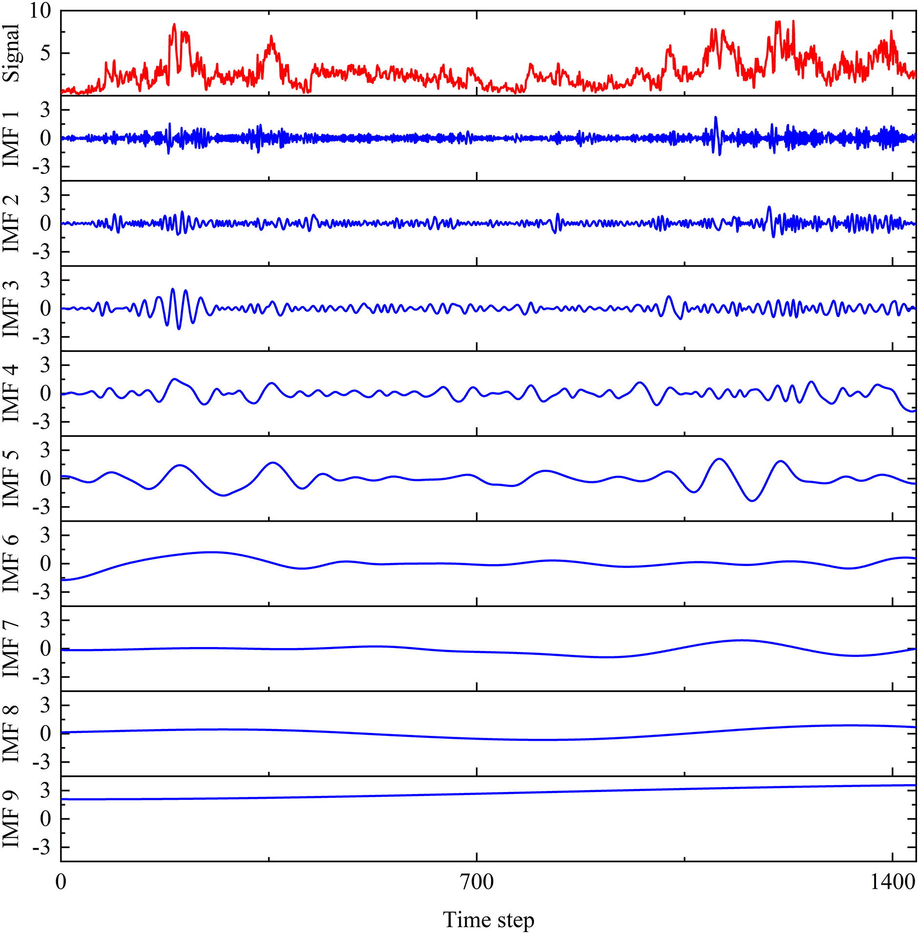
Figure 11: CEEMDAN output of average wind speed from 01 January to 10 January in 2015 (unit: m/s)
3.4 Feature Extraction Backbone Network
In the feature extraction process, an 18-layer residual network (ResNet-18) is employed as the backbone module to analyze the IMF signal bands. The main components of ResNet-18 are the Conv Blocks and the Identity Blocks, where the Conv Blocks are designed to shift the dimensionality of the network, and the Identity Blocks serve to extract features. Both the Conv Block and Identity Block can be accessed through a combination of three layers (Conv2D, BatchNorm and ReLU) preset by TensorFlow 2.0, as illustrated in Fig. 12.
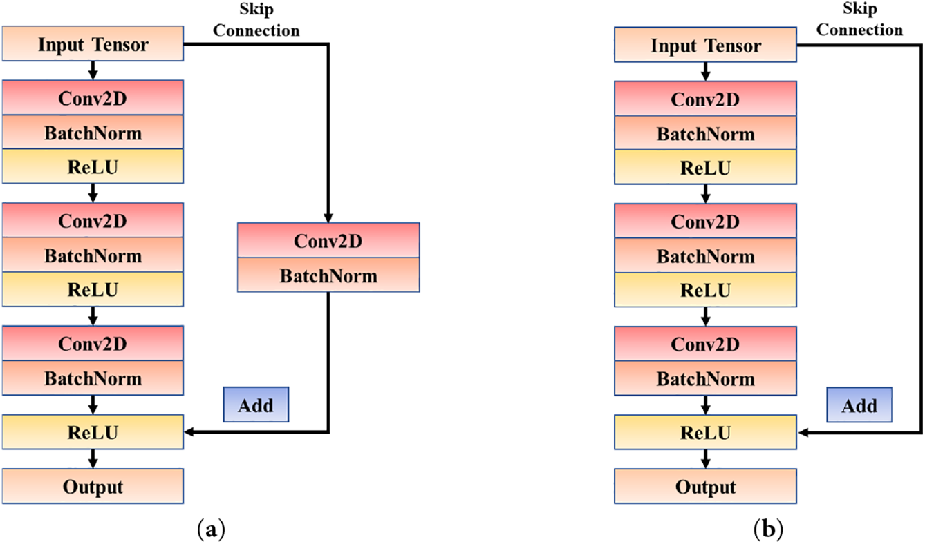
Figure 12: Typical Blocks in ResNet-18 model: (a) Conv Block; (b) Identity Block
The adoption of ResNet-18 achieves advantages in two different aspects. On the one hand, ResNet-18 employs a skip-connection mechanism, which can effectively suppress the problem of declining learning efficiency in deep networks [33]. On the other hand, as convolution advances, the perceptual field of kernels expands, allowing the neural network to have a comprehensive understanding of the signal band from local to global. Based on the superiority of ResNet-18, a convolutional method based on multi-scale feature fusion is proposed in this study, which is demonstrated in Fig. 13.
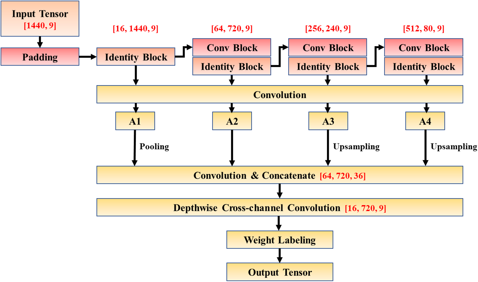
Figure 13: Proposed feature extraction backbone network
In the backbone network for feature extraction, a total of 9 sets of IMFs data, each consisting of 1440 timesteps, are fed into alternating Conv Blocks and Identity Blocks for further convolutional operations. The Conv Block is responsible for transforming the tensor dimension by adjusting the number of hidden layers and the stride length, and then passing the tensor into the Identity Block for feature extraction to obtain the initial convolution results
After the initial convolution results undergo dimensional normalization and are functionally stitched through up-sampling and pooling layers, the integration of channels is achieved using a Depth-wise convolution layer to obtain the feature output. Depth-wise convolution is an effective cross-channel convolution method, and many depth extraction networks developed in recent years, such as Xception and Mobile Net, have adopted this technique to depth extraction networks. Experiments have verified the efficiency of this method in extracting data features from high-dimensional tensors. Consequently, employing Depth-wise convolution to streamline the feature tensors contributes to the operational capacity and the reduction of computational costs.
Subsequently, an attention system is introduced for labeling the weights of the data extraction tensor. In the prediction process, the importance of wind speed at different timesteps and frequency components is inconsistent, hence the introduction of AM layers in the model that highlight key features can serve as guidance for the prediction module to undertake targeted learning. CBAM is a novel lightweight convolutional attention module that integrates channel attention mechanism and spatial attention mechanism by compressing dimensions through pooling layers, as demonstrated in Eqs. (10)–(12).
where
As the final step of the backbone network, the LSTM predictor processes the sequence of attention-weighted feature vectors generated by the convolutional backbone: at each timestep, it ingests the current feature vector along with its hidden and cell states, employs gated mechanisms (input, forget, and output gates) to update memory, and outputs a hidden-state sequence that captures both short-term fluctuations and long-range temporal dependencies accroding to Eqs. (13)–(15).
where
Owing to its architecture, the LSTM explicitly preserves and updates internal memory over time, making it well suited to transform the backbone spatial–spectral features into coherent multi-step forecasts. It learns how past feature patterns shape future values while attenuating irrelevant or noisy signals. The process of the LSTM-related layers is illustrated in Fig. 14.
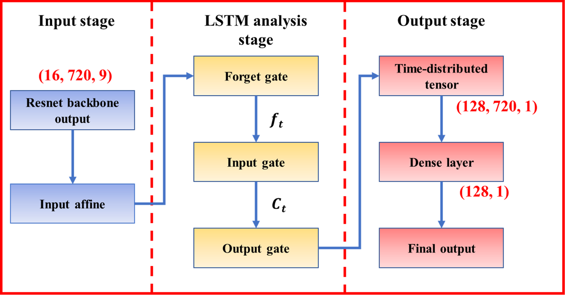
Figure 14: The framework of LSTM-related layers
Compared with a conventional shallow CNN–LSTM, the ResNet–LSTM architecture offers richer and more stable inputs to the recurrent predictor. The deep residual backbone extracts hierarchical, multi-scale temporal–spectral features and, when combined with attention, emphasizes informative components before sequence modelling; residual connections maintain trainability for deeper extractors and depth-wise/channel-efficient operations control parameter growth. In contrast, a shallow CNN provides a more limited receptive field and less expressive embeddings, which constrains the LSTM’s ability to model complex, multi-scale dependencies. Consequently, ResNet–LSTM typically achieves improved representational richness, forecast stability and transferability.
From the clustering results in Section 3.2, it is noted that the wind fields in Jena exhibit different characteristics depending on the wind direction, and each of these clustering results requires the training of a corresponding backbone network for feature extraction. Thus, problems may arise when a complete neural network training is performed for each of the clustering results as follows.
1. An excessive number of training iterations can lead to high training time and computational expenses.
2. The inability to share the primary feature extraction network for each clustering result causes a slowdown in the training performance and increases the storage space requirements.
3. The database available for training the backbone network within each cluster is reduced, rendering the network more difficult to be tuned, especially for clusters that contain limited time series.
To address these issues, transfer learning methods have been introduced to improve the efficiency and accuracy of backbone models. Transfer learning is a powerful machine learning approach that enables models to utilize what they have learnt from the previous dataset to perform new tasks. In this study, a backbone network applicable to a particular clustering result is first trained. Subsequently, a portion of the convolutional layers in the backbone network are frozen and implemented for the rest of the clustering results in accordance with the feature transfer approach, as shown in Fig. 15.
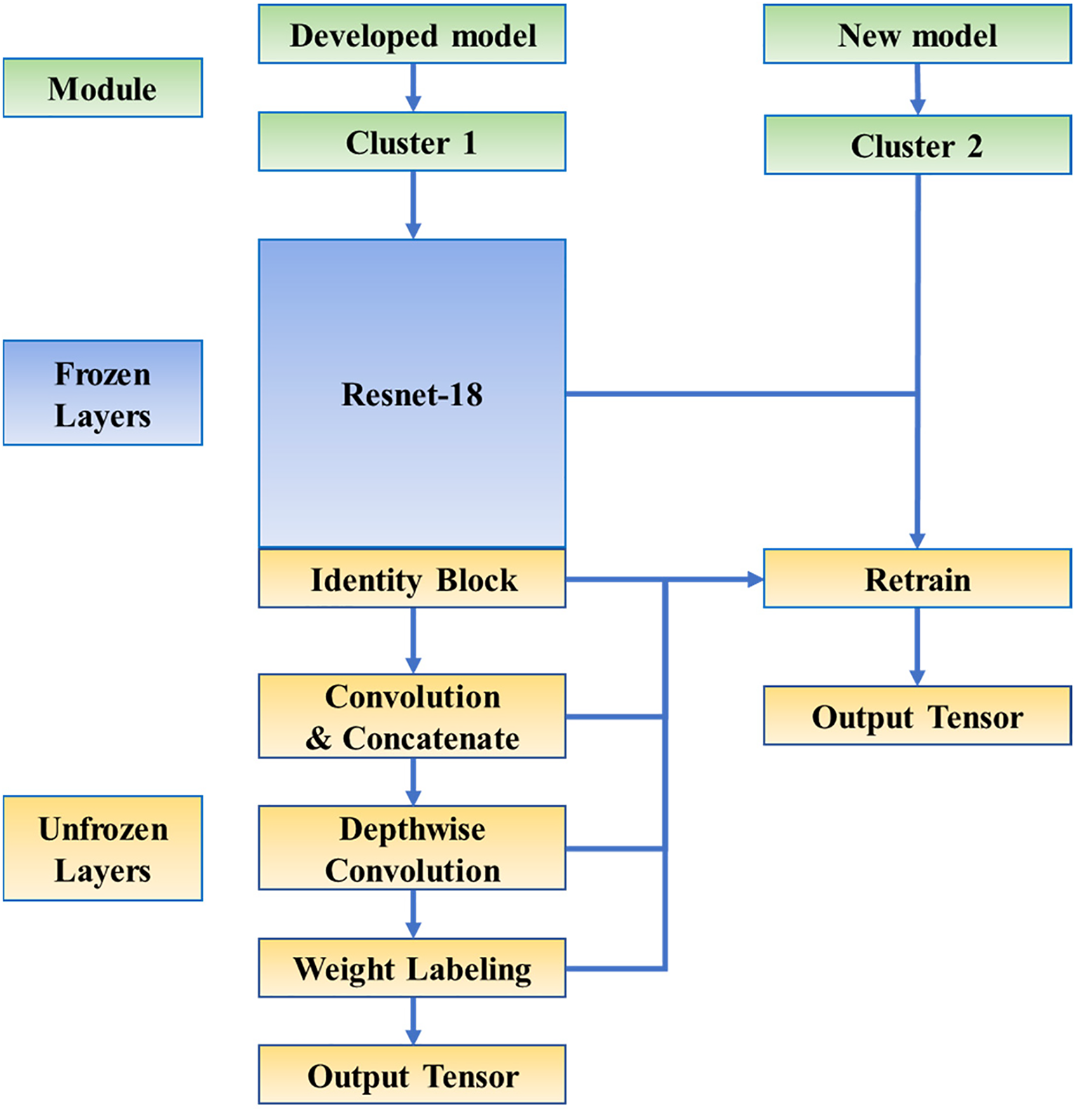
Figure 15: Transfer learning model construction diagram
As illustrated in Fig. 15, with the replacement of the clusters, the majority of the neural network is frozen and the weights are fixed in the new model. The retrained layers include the last Identity Block module of ResNet-18, the uniform dimensional convolution module, the cross-channel convolution module, and the weight labelling module. The model will be endowed with a finer learning rate and ends when the loss function converges after several training epochs.
4 Equations and Mathematical Expressions
The experiment settings encompass the following four aspects.
1. Hardware equipment. In this study the hardware device employed is a Dell workstation configured with a 3.60 GHz Intel Core i9-9900K processor. The workstation operates on Windows 10 and is equipped with a 16 GB RAM.
2. Dataset segmentation. The dataset includes 52,560 10-min average wind speed observations collected in Jena city throughout 2015. During the model training phase, sequential time series data spanning 10 days (1440 timesteps) are input into the model to predict wind speeds for the following 24 h (144 timesteps). Given the length of the time series data to be forecasted, a total of 50,977 wind speed samples can be generated from the dataset for training. The wind speed time series for each cluster are divided into three sets: the training set (40%), the validation set (30%), and the test set (30%). These sets are constructed through random sampling to avoid any bias from human factors. Fig. 16 provides a detailed breakdown of the dataset segmentation process.
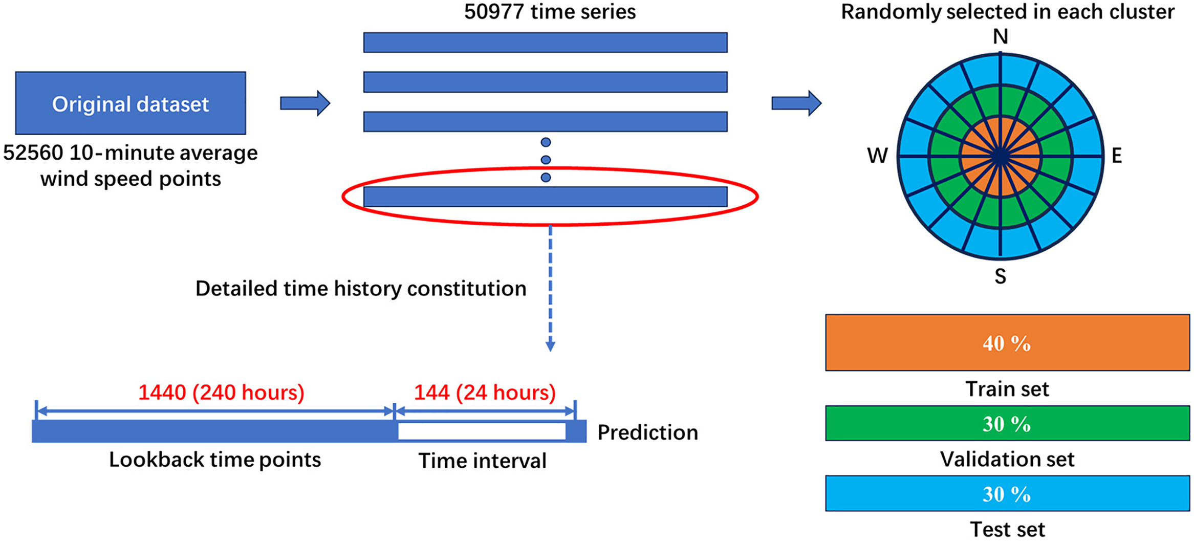
Figure 16: Breakdown of the dataset segmentation process
To address the data preprocessing requirements, this section describes the comprehensive preprocessing steps applied to the wind speed time series data. Normalization is performed using Min-Max scaling to standardize input features within the [0, 1] range, mitigating scale variations across datasets. Missing data points, identified during initial analysis, were handled via linear interpolation to maintain temporal continuity and dataset integrity.
3. Hyperparameters. The model proposed in the study is deployed in Anaconda and runs in the Python 3.7.11 virtual environment. The Adam optimizer and ReLU activation function are adopted for the deep learning module. For the model utilizes the fully training and the transfer training strategy, the learning rate is set to
4. Loss function. The loss function employed to assess the predictive efficacy of the model comprises three components: MAE (mean absolute error), RMSE (root mean squared error), and MAPE (mean absolute percentage error), which are calculated as Eqs. (16)–(18).
where
The selection of MAE, RMSE, and MAPE as composite loss metrics is methodologically justified to provide a comprehensive evaluation of wind speed forecasting performance. MAE offers a robust measure of average error magnitude with reduced sensitivity to outliers, RMSE penalizes large deviations more heavily through its squaring operation, and MAPE assesses relative accuracy, which is essential for operational planning. Together, this multi-faceted approach captures complementary dimensions of model precision, ensuring balanced optimization during training.
In this section, the prediction results of the proposed model for each cluster will be discussed in detail. The effectiveness of the accuracy-enhanced and efficiency-enhanced methods employed in the study, including the clustering sub-model, the prediction sub-model and the transfer learning sub-model, will be validated. In addition, the proposed model will be compared with the state-of-the-art mainstream models in terms of prediction accuracy metrics to demonstrate its superiority.
According to the study in Section 3.2, prediction models based on clustering results are developed, with a total of four wind speed models for Weibull-shaped distribution wind speed time series (
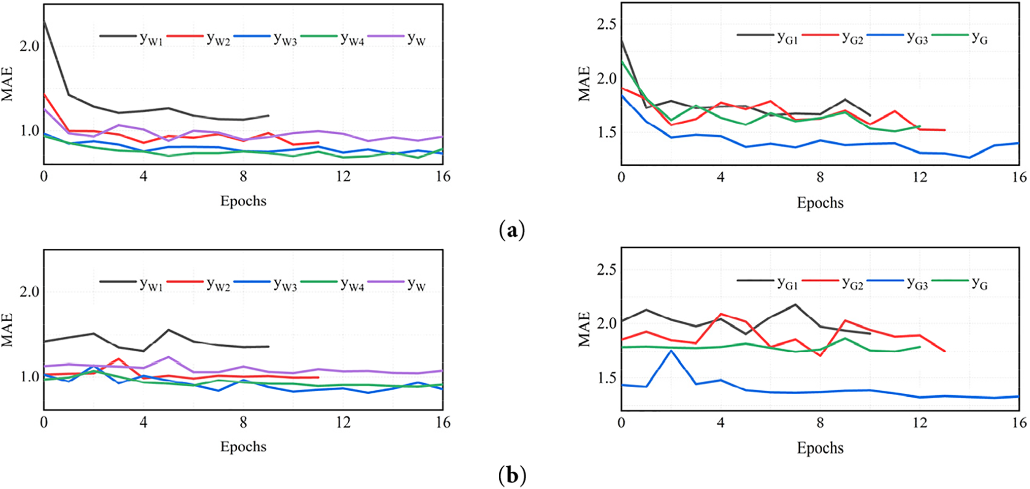
Figure 17: The convergence of model in training: (a) training set; (b) validation set
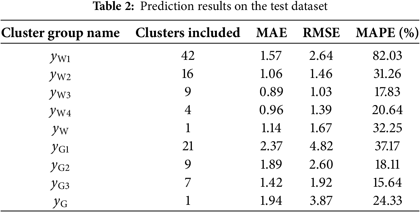
The predictions listed in Table 2 and Fig. 17 are the optimum results considering the effect of transfer learning (see Section 5.2). From the prediction results illustrated, it is noteworthy that:
1. In Fig. 17, the convergence curves of the loss function for all training sets display a consistent downward trend as the training progresses, both in the training and validation sets. This indicates that the designed model effectively addresses wind speed prediction challenges. Notably, the curves for
2. In the clustering models for Weibull-shaped distribution wind speed time series,
3. For the clustering of Gaussian-shaped distribution wind speed time series, the
4. Considering the prediction results for
To sum up the analysis provided above, it can be deduced that the model produces the most accurate wind speed prediction results in line with the clustering results
5.2 Assessment of Transfer Learning Effectiveness
In comparison to independently training a model for each distinct wind field cluster, transfer learning showcases a significant enhancement in both efficiency and precision. The efficiency can be gauged in terms of time taken for model training, denoted as Time, while maintaining uniform program conditions. Table 3 offers a ratio analysis of loss functions for independent training and transfer learning methods to facilitate a comprehensive comparison. Taking the MAE loss function as an example, the ratio is calculated as Eq. (19).
where
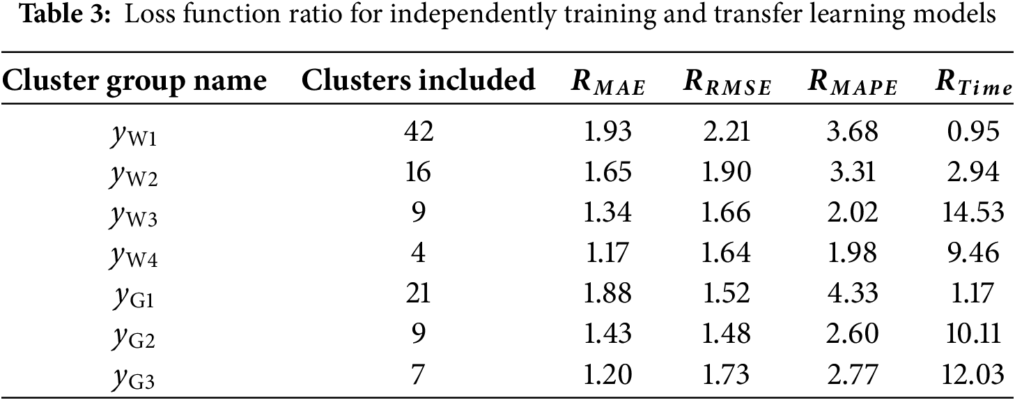
The
In addition, the
Subsequently, the training process of transfer learning should also be discussed. As illustrated in Fig. 15, the backbone network obtained by complete training on a particular cluster data, named the initial network in the study, can have a significantly implicate on the prediction accuracy of the model, hence investigation to the sequence of model training for transfer learning is worthwhile. For clusters
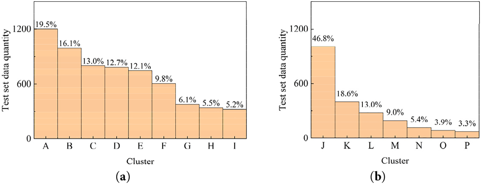
Figure 18: Diagram of the test set data distribution: (a) cluster result for
In Fig. 18, the study named the clusters according to the quantity of wind speed time series included. The clusters (A) to (I) correspond to the
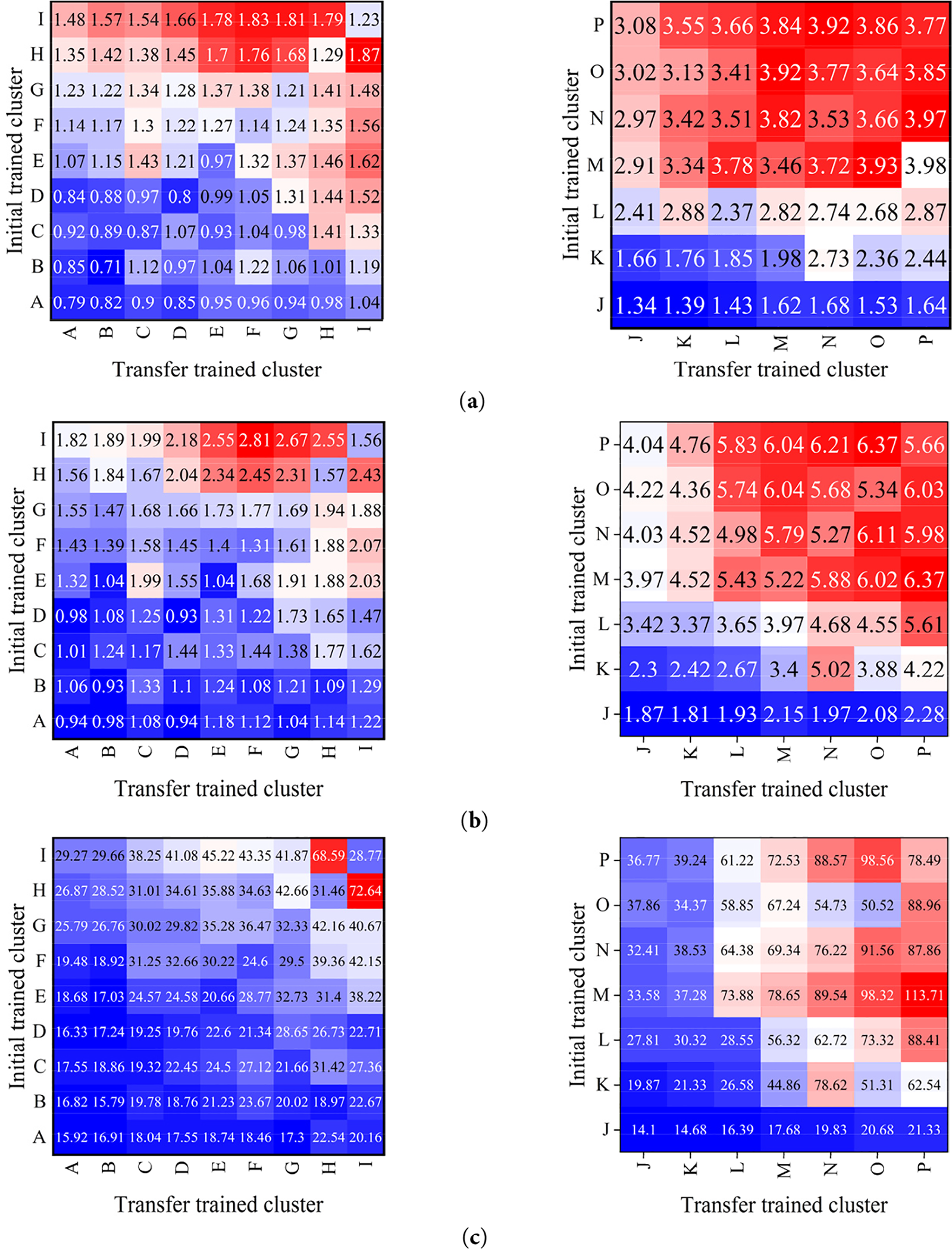
Figure 19: Transfer learning prediction results based on different initial models: (a) MAE loss function; (b) RMSE loss function; (c) MAPE loss function
From the listed results, it can be noted that the initial model training on the cluster where the main wind direction lies can ensure the adequacy of the training data and prevent overfitting, thus enabling the model set obtained by transfer learning to have better convergence and prediction accuracy. To further demonstrate the model performance, the prediction results obtained by transfer learning with clusters A and J as the initial models are presented in a scatter plot in Fig. 20. To facilitate comparison of the different clusters, the prediction results are normalized with the horizontal and vertical coordinates denoted by
where
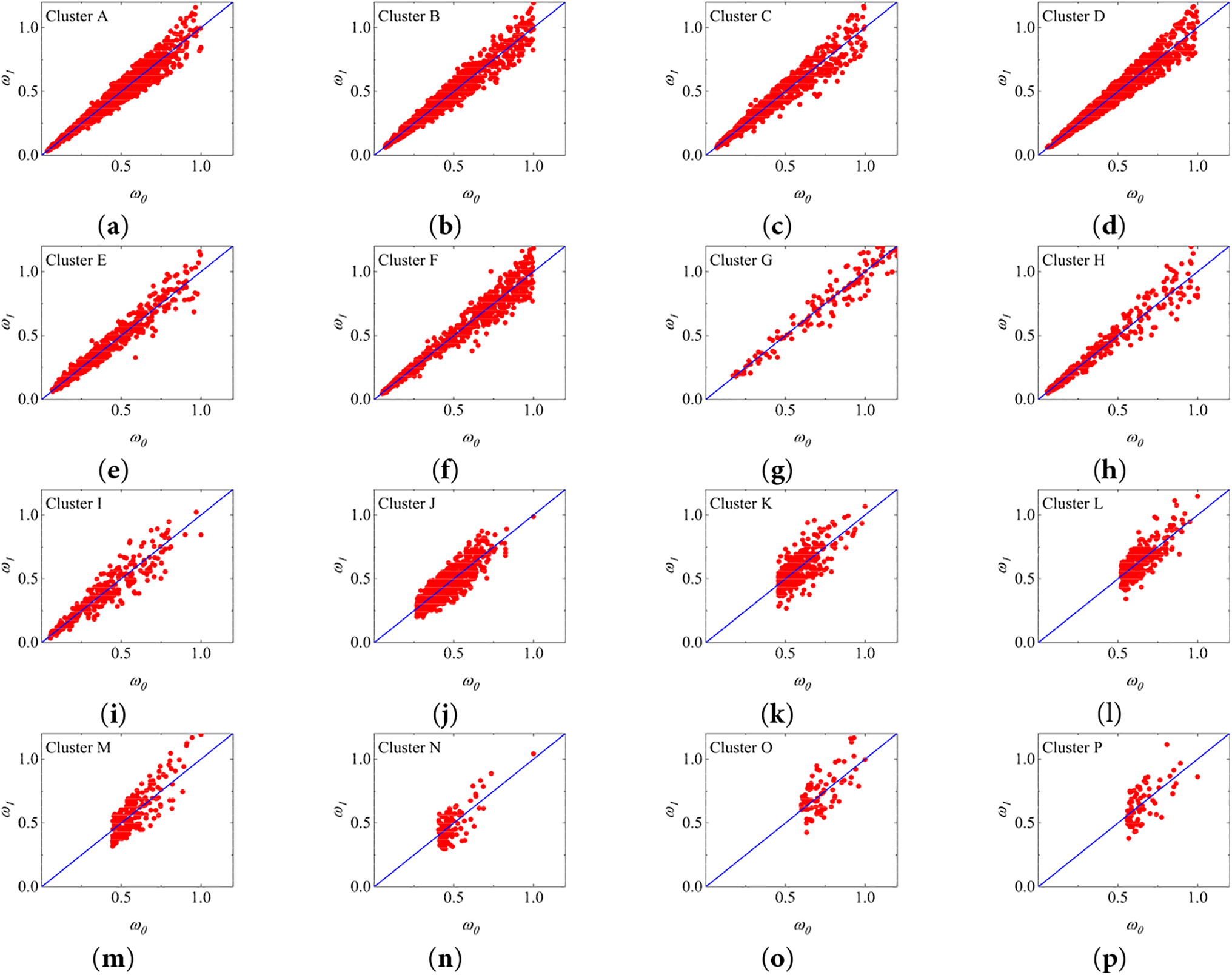
Figure 20: Wind speed prediction results with transfer learning in each cluster
According to Eqs. (20) and (21), with
5.3 Comparison with Baseline Models
For the purpose of objectively substantiating the advancement of the proposed models in terms of predictive capability, particularly the necessity of ResNet-18 and CBAM module for character extraction. A number of controlled commonly employed mainstream prediction models are outlined and applied to forecasts on
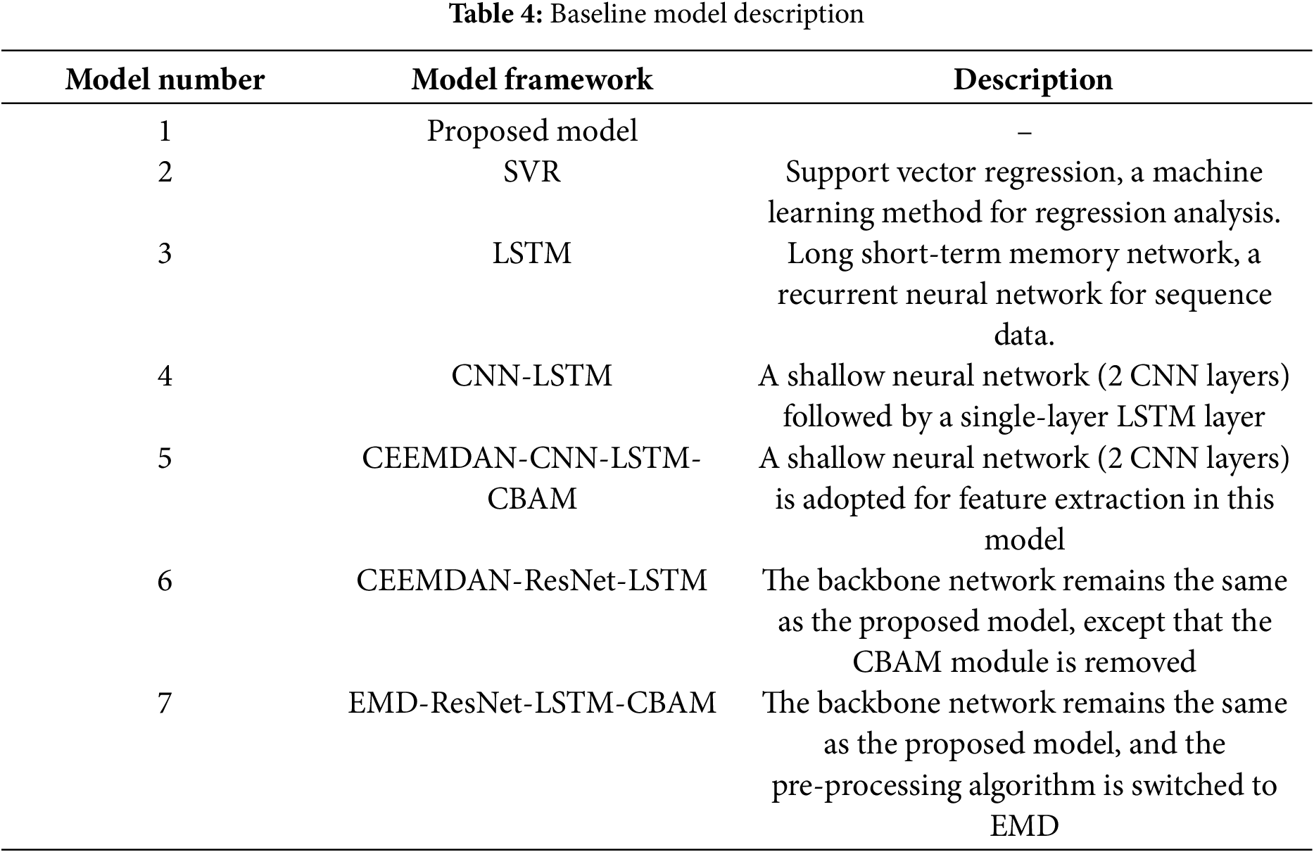
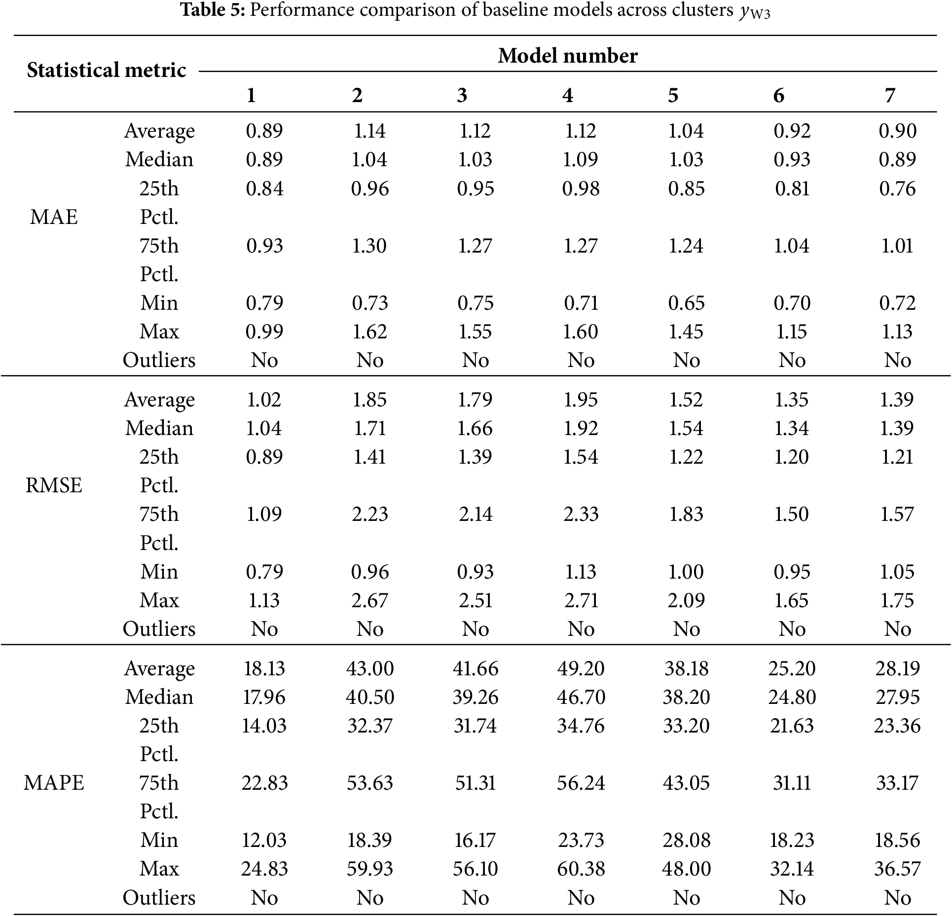
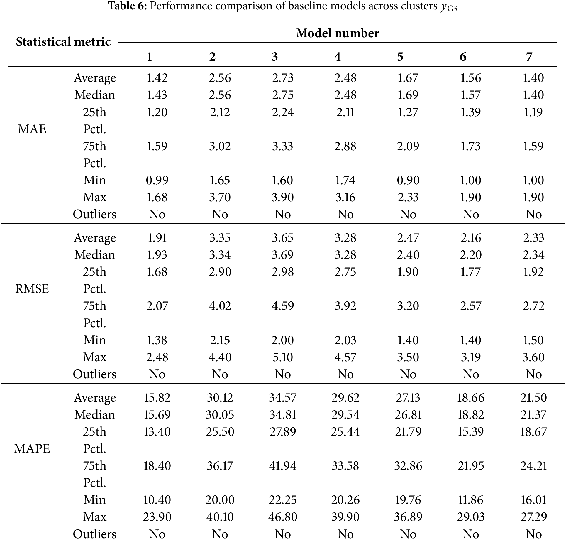
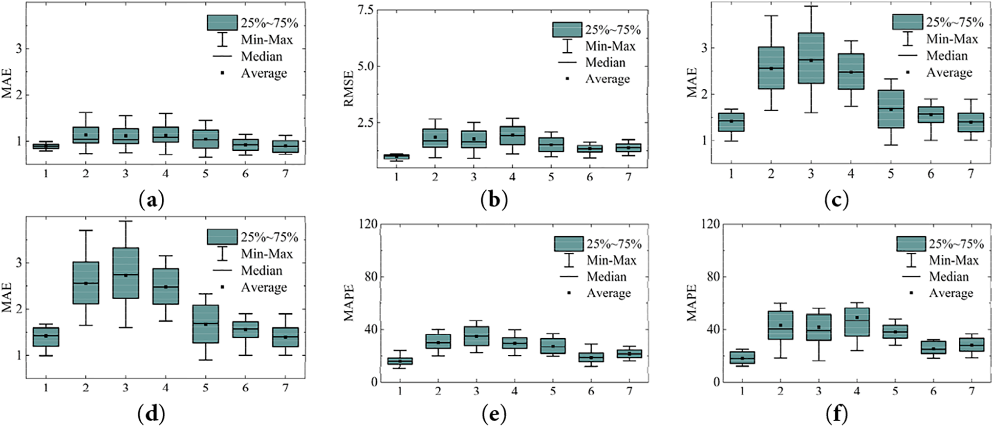
Figure 21: Predictive results of the baseline models: (a–c) for
It is worth noting the advantages of the proposed model from prediction results presented in Fig. 21 and Tables 5 and 6, which can be detailed for discussion in following aspects.
1. In the comparison among CNN-LSTM and proposed model, for the forecasting accuracy, the proposed model performs considerably better on all three loss functions MAE, MSE and MAPE, manifesting superiority over single feature extraction network and recurrent neural network in the case of 24 h ahead forecasting.
2. The forecast results from the CEEMDAN-CNN-LSTM-CBAM model highlight that the shallow CNN network falls short in meeting feature extraction demands owing to the restricted receptive field of the convolutional kernel in a network with insufficient layers. Consequently, the accuracy and stability of predictions do not match those of the proposed model.
3. The CEEMDAN-ResNet-LSTM model exhibits superior performance among the baseline models. However, without the CBAM attention mechanism, the prediction results lack stability during multiple prediction epochs. This model performance suggests that the incorporation of the attention mechanism can effectively enhance prediction stability and bolster the credibility of the model.
4. Compare with the proposed model, the EMD-ResNet-LSTM-CBAM model transitions from CEEMDAN to EMD for the preprocessing of wind speed data. Experimental results highlight the superiority of the CEEMDAN method in handling modal aliasing. The signal frequencies within each IMF band are more concentrated, facilitating the architecture of the feature extraction sub-model.
To statistically validate the difference in predictive accuracy between the proposed model and the baseline models, a paired t-test is conducted on the MAE results, with detailed outcomes presented in Tables 7 and 8. In the tables,
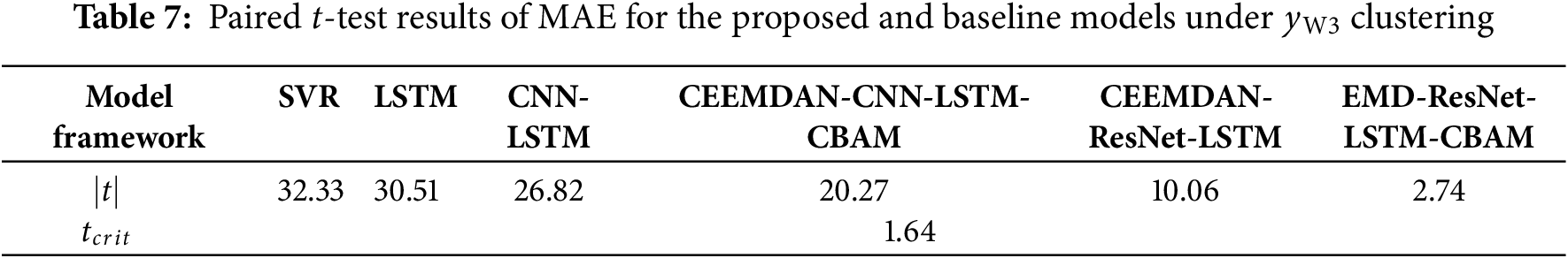
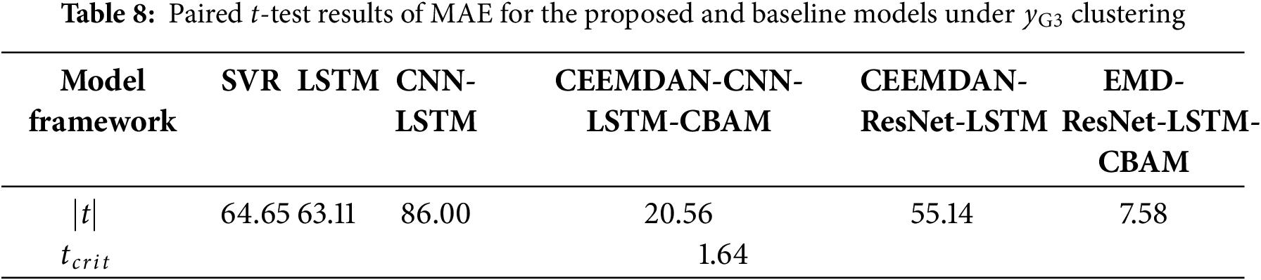
Tests are conducted on the MAE values for the output results of different models in Tables 7 and 8. The other two loss functions are not used because their distribution violated the normality assumption required for this test. The results show that, at the 95% confidence level, the predictive accuracy of the proposed model is statistically superior to that of all baseline models, suggesting that its enhanced predictive performance appears attributable to structural advantages rather than chance.
In accordance with the analysis in Section 5, it is possible to verify the predictive credibility of the proposed model established on the 2015 wind speed time series dataset for the city of Jena. However, the generalizability of the model to interannual time datasets remains unverified, thus challenging to verify whether the model enables support for long-term forecasting of local wind speeds. To validate the robustness of the predicting results on local wind field over long period, the proposed model is applied to the wind speed time series dataset for the following year with a restricted number of training epochs. After three additional training epochs for each cluster, the prediction results of the model on the test set are presented in Table 9. Furthermore, the results of four randomly selected time series predictions for a duration of 12 h are presented in Fig. 22.
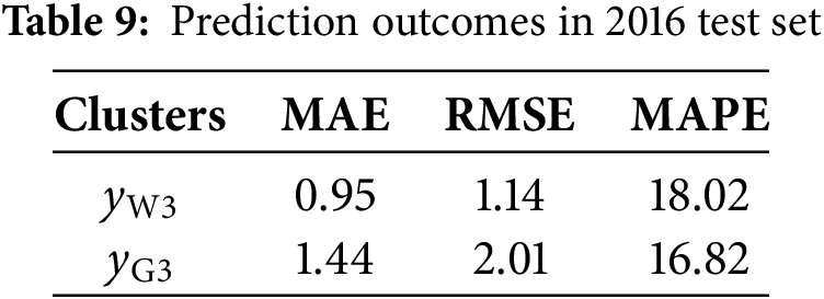
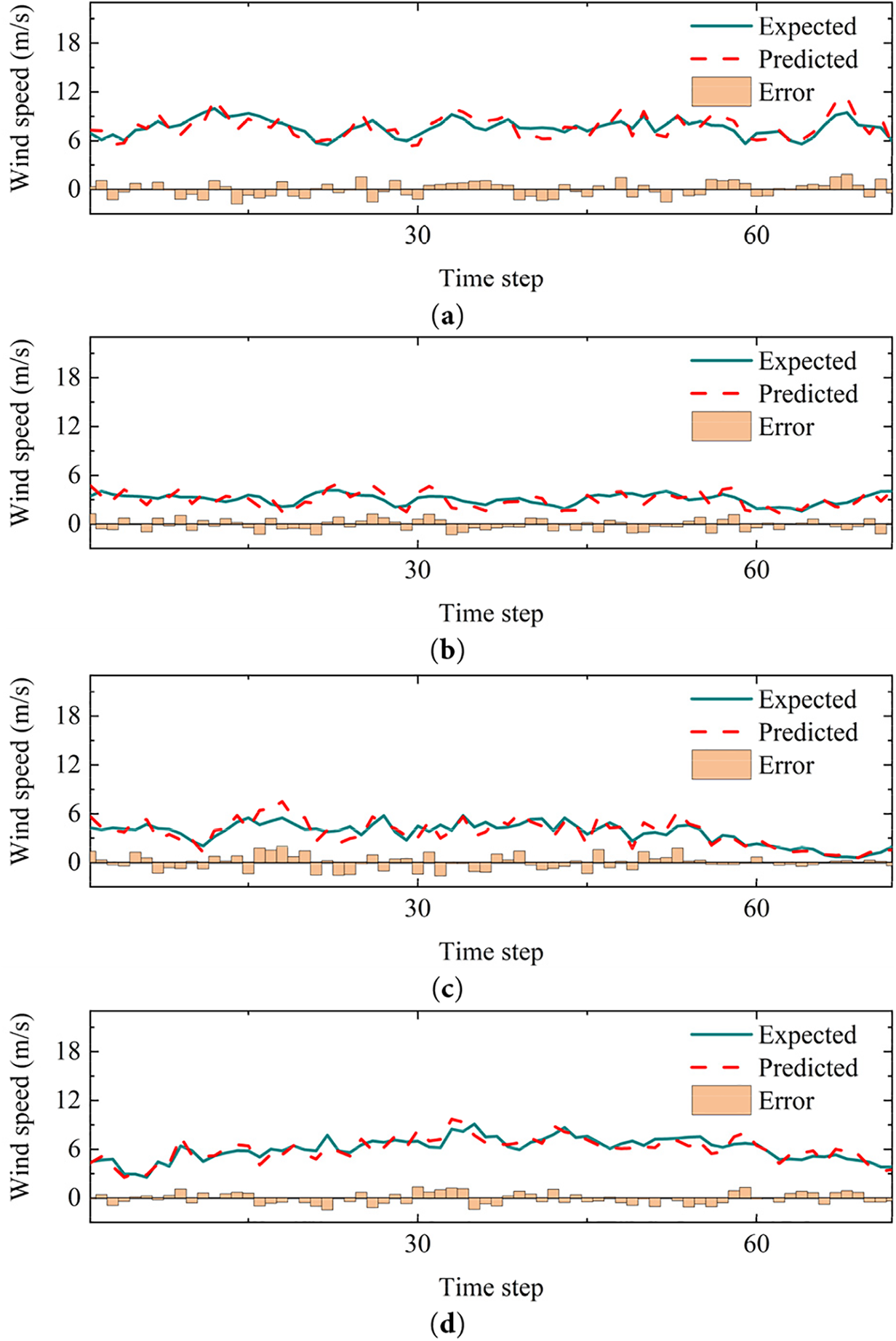
Figure 22: Time series forecast on 2016 wind speed time series dataset
In the context of the overall prediction results in the 2016 wind speed time series dataset, the overall prediction results maintain appreciable accuracy despite limiting the number of training epochs. This performance demonstrates the strong generalization capability of the model to local wind field attributes and affirms the consistency of forecast accuracy in prolonged prediction processes. Fig. 22 depicts the prediction outcomes that further substantiate the efficacy of the proposed model in forecasting wind speed trends across varying wind speed scenarios.
In the context of the overall prediction results in the 2016 wind speed time series dataset, the overall prediction results maintain appreciable accuracy despite limiting the number of training epochs. This performance demonstrates the strong generalization capability of the model to local wind field attributes and affirms the consistency of forecast accuracy in prolonged prediction processes. Fig. 22 depicts the prediction outcomes that further substantiate the efficacy of the proposed model in forecasting wind speed trends across varying wind speed scenarios.
This study proposes a novel hybrid machine learning model for 24-h wind speed prediction by combining wind field clustering, deep feature extraction, and transfer learning. The key findings are as follows:
(1) By utilizing wind speed distribution and power spectral density (PSD) properties, the clustering of wind speed time series effectively alleviates model generalization challenges and enhances physical interpretability. The DB-SCAN clustering method revealed that the optimal clustering result depends on balancing the number of clusters and the amount of data in each cluster. Multiple clustering schemes may be encountered during this process, underscoring the need for careful consideration of data distribution.
(2) Transfer learning significantly improves model efficiency and accuracy. It proves especially useful for clusters with limited data, effectively addressing overfitting and enhancing prediction precision. The study demonstrates that selecting clusters based on the main wind direction for initial model training is an effective strategy for transfer learning.
(3) The ResNet module excels in convolving time series data across multiple perceptual domains, thoroughly extracting IMF (Intrinsic Mode Function) signals through up-sampling and depth-wise layers. This method outperforms shallow CNNs (convolutional neural networks) in feature acquisition. Additionally, the CBAM (Convolutional Block Attention Module) improves the robustness of predictions by reducing the dispersion of errors, leading to more reliable outcomes.
(4) The prediction results on the 2016 wind speed dataset confirm the robustness and strong generalization capability of the model. The model effectively predicts wind speeds after a short training period, demonstrating its ability to provide accurate forecasts over extended periods.
The wind speed prediction model proposed in this study still has some limitations, and further research will be conducted in the future to address the following aspects:
(1) Consideration can be given to introducing a confidence interval sub-model to mitigate prediction uncertainty. This sub-model involves analyzing confidence intervals, allowing the model to provide not only wind speed values but also plausible range for wind speed changes.
(2) The PSO (Particle Swarm Optimization) parameter optimization was not fully explored in this study. While PSO is effective for optimizing the model’s parameters, its performance depends on settings like the number of particles and iteration limits. In the future, we will improve the PSO process by adjusting its parameters dynamically, leading to better results and faster convergence.
(3) The model demonstrates robust generalization within studied wind regimes, but requires validation under varying weather, geographical conditions, and seasonal patterns. Future work will develop a cross-regional framework using multi-climate data to quantify adaptation limits. We will implement adaptive transfer learning that dynamically adjusts feature extraction based on atmospheric diagnostics, enabling forecasting across diverse scenarios. The revised research roadmap progresses through three strategically phased objectives: Short-term efforts (0–6 months) will conduct sensitivity analysis to quantify model resilience boundaries across key meteorological parameters. Mid-term work (7–12 months) will validate operational robustness via multi-scale regional testing under real-world constraints. The long-term objective (13–18 months) will implement full integration with numerical weather prediction systems, culminating in an adaptive framework that enables synergistic data assimilation for complex climate forecasting scenarios while achieving systematic cross-environment validation as identified in the limitations.
Acknowledgement: The financial supports from Science and Technology Research and Development Program Project of China Railway Group Limited (No. 2023-Major-02), National Natural Science Foundation of China (Grant No. 52378200), and Sichuan Science and Technology Program (Grant No. 2024NSFSC0017) are highly appreciated. All the opinions presented here are those of the writers, not necessarily representing those of the sponsors.
Funding Statement: This research was funded by Science and Technology Research and Development Program Project of China Railway Group Limited (No. 2023-Major-02), National Natural Science Foundation of China (Grant No. 52378200) and Sichuan Science and Technology Program (Grant No. 2024NSFSC0017).
Author Contributions: Investigation, Weiqi Mao; Data curation, Weiqi Mao; Methodology, Enbo Yu; Funding acquisition, Guoji Xu; Formal analysis, Enbo Yu; Resources, Guoji Xu; Supervision, Xiaozhen Li; Project administration, Xiaozhen Li; Writing—original draft preparation, Weiqi Mao; Writing—review and editing, Enbo Yu and Guoji Xu. All authors reviewed the results and approved the final version of the manuscript.
Availability of Data and Materials: The data that support the findings of this study are openly available in open-source online data repository hosted by Max Planck Institute for Biogeochemistry at https://www.bgc-jena.mpg.de/wetter (accessed on 31 August 2025).
Ethics Approval: Not applicable.
Conflicts of Interest: The authors declare no conflicts of interest to report regarding the present study.
References
1. Ahmad T, Manzoor S, Zhang D. Forecasting high penetration of solar and wind power in the smart grid environment using robust ensemble learning approach for large-dimensional data. Sustain Cities Soc. 2021;75:103269. doi:10.1016/j.scs.2021.103269. [Google Scholar] [CrossRef]
2. Saeed A, Li C, Gan Z, Xie Y, Liu F. A simple approach for short-term wind speed interval prediction based on independently recurrent neural networks and error probability distribution. Energy. 2022;238(3):122012. doi:10.1016/j.energy.2021.122012. [Google Scholar] [CrossRef]
3. Ponnuswamy P, Palaniappan SC. Prediction of wind energy location by parallel programming using MPI-based KMEANS clustering algorithm. Energy Sources Part A Recovery Util Environ Eff. 2024;46(1):5451–73. doi:10.1080/15567036.2024.2334923. [Google Scholar] [CrossRef]
4. Wang J. A hybrid wavelet transform based short-term wind speed forecasting approach. Sci World J. 2014;2014(3, article 1):914127. doi:10.1155/2014/914127. [Google Scholar] [PubMed] [CrossRef]
5. Zhang N, Xue X, Jiang W, Shi L, Feng C, Gu Y. A novel hybrid forecasting system based on data augmentation and deep learning neural network for short-term wind speed forecasting. J Renew Sustain Energy. 2021;13(6):066101. doi:10.1063/5.0062790. [Google Scholar] [CrossRef]
6. Zhao Z, Yun S, Jia L, Guo J, Meng Y, He N, et al. Hybrid VMD-CNN-GRU-based model for short-term forecasting of wind power considering spatio-temporal features. Eng Appl Artif Intell. 2023;121(4610):105982. doi:10.1016/j.engappai.2023.105982. [Google Scholar] [CrossRef]
7. Galanis G, Papageorgiou E, Liakatas A. A hybrid Bayesian Kalman filter and applications to numerical wind speed modeling. J Wind Eng Ind Aerodyn. 2017;167(3):1–22. doi:10.1016/j.jweia.2017.04.007. [Google Scholar] [CrossRef]
8. Hur SH. Short-term wind speed prediction using extended Kalman filter and machine learning. Energy Rep. 2021;7(114137):1046–54. doi:10.1016/j.egyr.2020.12.020. [Google Scholar] [CrossRef]
9. Wang H, Zhang YM, Mao JX. Sparse Gaussian process regression for multi-step ahead forecasting of wind gusts combining numerical weather predictions and on-site measurements. J Wind Eng Ind Aerodyn. 2022;220:104873. doi:10.1016/j.jweia.2021.104873. [Google Scholar] [CrossRef]
10. Tian Z. Short-term wind speed prediction based on LMD and improved FA optimized combined kernel function LSSVM. Eng Appl Artif Intell. 2020;91(2):103573. doi:10.1016/j.engappai.2020.103573. [Google Scholar] [CrossRef]
11. Ren Y, Wen Y, Liu F, Zhang Y. A short-term wind speed prediction method based on interval type 2 fuzzy model considering the selection of important input variables. J Wind Eng Ind Aerodyn. 2022;225(1):104990. doi:10.1016/j.jweia.2022.104990. [Google Scholar] [CrossRef]
12. Niu Y, Wang J, Zhang Z, Yu Y, Liu J. A combined interval prediction system based on fuzzy strategy and neural network for wind speed. Appl Soft Comput. 2024;155(4):111408. doi:10.1016/j.asoc.2024.111408. [Google Scholar] [CrossRef]
13. Wang J, Niu W, Yang Y. Wind turbine output power prediction by a segmented multivariate polynomial-XGBoost model. Energy Sources Part A Recovery Util Environ Eff. 2024;46(1):505–21. doi:10.1080/15567036.2023.2284840. [Google Scholar] [CrossRef]
14. Sun W, Wang X, Tan B. Multi-step wind speed forecasting based on a hybrid decomposition technique and an improved back-propagation neural network. Environ Sci Pollut Res Int. 2022;29(33):49684–99. doi:10.1007/s11356-022-19388-4. [Google Scholar] [PubMed] [CrossRef]
15. Lu P, Ye L, Tang Y, Zhao Y, Zhong W, Qu Y, et al. Ultra-short-term combined prediction approach based on kernel function switch mechanism. Renew Energy. 2021;164(2):842–66. doi:10.1016/j.renene.2020.09.110. [Google Scholar] [CrossRef]
16. Ma Z, Chen H, Wang J, Yang X, Yan R, Jia J, et al. Application of hybrid model based on double decomposition, error correction and deep learning in short-term wind speed prediction. Energy Convers Manag. 2020;205(1):112345. doi:10.1016/j.enconman.2019.112345. [Google Scholar] [CrossRef]
17. Zhang W, Qu Z, Zhang K, Mao W, Ma Y, Fan X. A combined model based on CEEMDAN and modified flower pollination algorithm for wind speed forecasting. Energy Convers Manag. 2017;136(995):439–51. doi:10.1016/j.enconman.2017.01.022. [Google Scholar] [CrossRef]
18. Peng T, Zhou J, Zhang C, Zheng Y. Multi-step ahead wind speed forecasting using a hybrid model based on two-stage decomposition technique and AdaBoost-extreme learning machine. Energy Convers Manag. 2017;153(8):589–602. doi:10.1016/j.enconman.2017.10.021. [Google Scholar] [CrossRef]
19. Cai H, Jia X, Feng J, Li W, Hsu YM, Lee J. Gaussian process regression for numerical wind speed prediction enhancement. Renew Energy. 2020;146:2112–23. doi:10.1016/j.renene.2019.08.018. [Google Scholar] [CrossRef]
20. Ruiz-Aguilar JJ, Turias I, González-Enrique J, Urda D, Elizondo D. A permutation entropy-based EMD-ANN forecasting ensemble approach for wind speed prediction. Neural Comput Appl. 2021;33(7):2369–91. doi:10.1007/s00521-020-05141-w. [Google Scholar] [CrossRef]
21. He J, Yu C, Li Y, Xiang H. Ultra-short term wind prediction with wavelet transform, deep belief network and ensemble learning. Energy Convers Manag. 2020;205:112418. doi:10.1016/j.enconman.2019.112418. [Google Scholar] [CrossRef]
22. Han Y, Mi L, Shen L, Cai CS, Liu Y, Li K. A short-term wind speed interval prediction method based on WRF simulation and multivariate line regression for deep learning algorithms. Energy Convers Manag. 2022;258(1):115540. doi:10.1016/j.enconman.2022.115540. [Google Scholar] [CrossRef]
23. Zhou H, Zhang S, Peng J, Zhang S, Li J, Xiong H, et al. Informer: beyond efficient transformer for long sequence time-series forecasting. Proc AAAI Conf Artif Intell. 2021;35(12):11106–15. doi:10.1609/aaai.v35i12.17325. [Google Scholar] [CrossRef]
24. Liu HI, Galindo M, Xie H, Wong LK, Shuai HH, Li YH, et al. Lightweight deep learning for resource-constrained environments: a survey. ACM Comput Surv. 2024;56(10):1–42. doi:10.1145/3657282. [Google Scholar] [CrossRef]
25. Shi J, Wang S, Qu P, Shao J. Time series prediction model using LSTM-Transformer neural network for mine water inflow. Sci Rep. 2024;14(1):18284. doi:10.1038/s41598-024-69418-z. [Google Scholar] [PubMed] [CrossRef]
26. Pei C, Bao Y, Zhang X, Cheng X, Feng J. A CNN-LSTM model for predicting wind speed in non-stationary wind fields in mountainous areas based on wavelet transform and adaptive programming. AIP Adv. 2024;14(11):115009. doi:10.1063/5.0230026. [Google Scholar] [CrossRef]
27. Alamatsaz N, Tabatabaei L, Yazdchi M, Payan H, Alamatsaz N, Nasimi F. A lightweight hybrid CNN-LSTM explainable model for ECG-based arrhythmia detection. Biomed Signal Process Control. 2024;90(1):105884. doi:10.1016/j.bspc.2023.105884. [Google Scholar] [CrossRef]
28. Madlener R, Glensk B, Gläsel L. Optimal timing of onshore wind repowering in Germany under policy regime changes: a real options analysis. Energies. 2019;12(24):4703. doi:10.3390/en12244703. [Google Scholar] [CrossRef]
29. Wang Y, Li Y, Zou R, Song D. Bayesian infinite mixture models for wind speed distribution estimation. Energy Convers Manag. 2021;236(3):113946. doi:10.1016/j.enconman.2021.113946. [Google Scholar] [CrossRef]
30. Ozay C, Celiktas MS. Statistical analysis of wind speed using two-parameter Weibull distribution in Alaçatı region. Energy Convers Manag. 2016;121(9):49–54. doi:10.1016/j.enconman.2016.05.026. [Google Scholar] [CrossRef]
31. Chen X, Guo J, Tang H, Li Y, Wang L. Non-uniform wind environment in mountainous terrain and aerostatic stability of a bridge. Wind Struct. 2020;30(6):649–62. doi:10.12989/was.2020.30.6.649. [Google Scholar] [CrossRef]
32. Yu C, Li Y, Zhang M, Zhang Y, Zhai G. Wind characteristics along a bridge catwalk in a deep-cutting gorge from field measurements. J Wind Eng Ind Aerodyn. 2019;186(December 2017):94–104. doi:10.1016/j.jweia.2018.12.022. [Google Scholar] [CrossRef]
33. Shafiq M, Gu Z. Deep residual learning for image recognition: a survey. Appl Sci. 2022;12(18):8972. doi:10.3390/app12188972. [Google Scholar] [CrossRef]
Cite This Article
 Copyright © 2026 The Author(s). Published by Tech Science Press.
This work is licensed under a Creative Commons Attribution 4.0 International License , which permits unrestricted use, distribution, and reproduction in any medium, provided the original work is properly cited.
 Downloads
 Citation Tools