1 Introduction
The late stage of liver disease, known as liver cirrhosis, occurs when the liver organ fails to function correctly due to the possible transformation of healthy liver tissue into scar tissue caused by alcohol processing stress or viral infections. In the world, cirrhosis is responsible for one million fatalities annually, indicating its significant morbidity and mortality rates [1]. Ultimately, a chronic or continual injury causes the liver to slowly languish and become incapable of functioning properly. A distinctive feature of the liver is its ability to regenerate; however, this process is also inhibited by liver cirrhosis. Hepatitis B and C virus infections, prolonged alcohol consumption, other liver illnesses and disorders can all lead to cirrhosis. The risk of developing cirrhosis is higher in those with chronic viral infections [2]. Although before the extensive liver damage, the liver cirrhosis has no apparent symptoms. Hepatitis B is a major worldwide health concern, caused by a virus called hepatitis B. Fever, fatigue, joint pain, loss of appetite, nausea, vomiting, and jaundice may occur two weeks later as symptoms. An incubation period of 45−180 days (average 60−90 days) meant that many of the infected would not experience symptoms. Mother-to-child transmission and contact with contaminated bodily fluids such as blood, saliva, vaginal secretions, and semen are potential transmission modes [3,4]. In 2022, the World Health Organization estimates that 254 million individuals have a chronic hepatitis B infection, with 1.2 million new cases reported annually. An estimated 1.1 million people died mostly from cirrhosis and hepatocellular carcinoma (HCC) as a result of hepatitis B in 2022 [5]. Another significant risk factor for the development of chronic liver cirrhosis is heavy alcohol use, with 38% of adults over 15 years, consuming more than 17 liters of pure alcohol per year [6]. The prevalence of cirrhosis is approximately 10 to 20 percent of heavy drinkers after ten or more years, especially in individuals taking at least 50 grams of pure alcohol daily over 10 to 20 years, and there is a high degree of risk of fast liver destruction when alcohol intake is combined with HBV infection [7]. However, a lot of studies have demonstrated that the risk of developing cirrhosis is not increased if people do not consume more than 50 grams of pure alcohol daily. Consuming more than 50 grams of pure alcohol per day, however, speeds up the development towards liver cirrhosis in chronic hepatitis B carriers for both men as well as women. It is poisonous and fatal if a person weighing 60 kg takes in more than 300 grams of alcohol daily [8–10]. Hepatitis B effective vaccine available with 95% effective antibodies [11]. Chronic infection treatment is crucial to reduce the risk of severe problems like liver cancer or cirrhosis. Treatment duration varies depending on the genotype and medication used, ranging from six months to a year [12].
In studying the dynamical behavior of epidemic models, the incidence rates play a vital role. Capasso and Serio [13], for the first time, proposed the idea of saturation incidence rate β(A)SI1+α2I. In a population that is completely susceptible to the illness, β(A)I1+α2I achieves the saturation level when I grows and α2I measures the force of infection after entering the disease. In this incidence rate 11+α2I measures the inhibitory impact of behavioral changes in susceptible people when the number of infected people rises or the crowding effect of infective individuals. Compared to bilinear, the saturated incidence rate is more general.
The dynamical behavior of infectious illnesses, such as cholera, liver cirrhosis, Hepatitis B infection, and others, is commonly studied using mathematical models. Apart from modelling of infectious diseases, various research has also been done for anticancer medication and locating numbers [14,15]. Mathematical models are considered to be the tool helping to discuss hypotheses, verify the experiments, and simulate the dynamics of complex objects. Zhou and Fan [16] created an SIR (Susceptible-Infective-Recovered) model for susceptibility, infection, and recovery analysis to evaluate human behavior during medical resource shortages. Ilhan and Sahin have used the Morgan-Voyce collocation method (M-VCM) to determine the approximate solution of the SIR model with the vaccination effect. Their paper provides an alternative criterion of the certainty of the approximate solutions. They primarily tried to determine the exact solutions of the SIR model of vaccination [17]. Researchers have developed multiple models to study relationships between alcohol abuse patterns alongside cirrhosis evolution and hepatitis B virus infection processes. Park et al. [18] investigated the factors linked to alcohol consumption among Hepatitis B carriers in Korea and concluded that hazardous alcohol consumption is defined as consuming more than sixty grams of alcohol on one occasion for males or forty grams of alcohol on several occasions for females. A continuous and a discrete mathematical model were developed by Khajji et al. [19] to investigate the dynamical behavior of alcohol use and the effects of both public and private addiction treatment centers. By utilizing a mathematical model and an optimum control technique [20,21] elucidated the dynamics of infectious diseases and came to the conclusion that the illness may be controlled by vaccination and treatment. Zhou et al. [22] compared moderate and excessive drinking and came to the conclusion that moderate alcohol consumption has no discernible impact on the progression of liver cirrhosis, whereas excessive drinking causes liver inflammation in patients with chronic Hepatitis B infection, ultimately accelerating the progression of the disease. A mathematical model developed by Dano et al. [23], consisting of four classes, namely susceptible, acutely infected, cirrhotic, and recovered, with a logistic model to study the combined effect of Hepatitis B infection and heavy alcohol consumption on liver cirrhosis progression dynamics.
The novelty of our research is considering the effect of exposed and treated classes. Since Hepatitis B has a latent phase, and treatment effects. With the inclusion of the exposed class, a latent period is introduced, which delays the transmission of individuals into the acutely infected class. We assumed that a fraction of individuals move from the exposed to the recovered compartment directly. The treated class is included to model the impact of medical interventions, which helps in analyzing how treatment reduces the infectious (both acutely infected and cirrhotic) population and reduces the progression to liver cirrhosis. Moreover, the existence of a unique solution for the proposed model is examined, which is ignored in most of the papers. Furthermore, we used a saturated incidence rate to study the saturation effects. Two basic reproductive numbers are calculated when the minimum and maximum amount of pure alcohol is consumed, respectively. The 3D analysis of these basic reproductive numbers are also carried out. To the author’s utmost knowledge, no one has yet considered the same.
We organized this research study as follows. The model formulation, description, as well as associated assumptions are presented in Section 2. In Section 3, the qualitative analysis of the proposed model is presented. That is, the solution is of existence, uniqueness, positivity, as well as boundedness. Moreover, the feasible region is defined, equilibrium points, the basic reproductive number with 3D-type simulation, and local and global asymptotic stability at equilibria are calculated. In Section 4, the bifurcation phenomena are analyzed, where we proved the existence of forward bifurcation of the proposed model. The sensitivity analysis is carried out in Section 5, while the numerical simulations are explored in Section 7, and the conclusion is presented in Section 8.
2 Model Formulation
The total human population is denoted by N(t) and partitioned into six different compartments namely the susceptible, exposed, acutely infected, liver cirrhotic, treated and recovered denoted by S(t), E(t), I(t), C(t), T(t) and R(t), respectively. The susceptible individuals S(t) include those who are at risk of becoming infected but have not yet been infected at time t. People in the susceptible group are not immune to a possible infection. The exposed compartment E(t) includes those individuals who are infected but not yet infectious, meaning that they are in the incubation period, which implies that in their bodies the pathogen is present and replicating, but they are not capable of transmitting the disease to others. The population with acute infection I(t) is those who are currently infected with the disease, have developed a robust enough immunity to eradicate the disease from their bodies, and have the ability to transmit the disease to others. People with liver cirrhosis C(t) are asymptomatic infection individuals with end-stage liver disease who are capable of spreading the disease at any time t. Treated compartment T(t) includes those individuals who do not have enough immunity to clear the disease from their bodies; therefore, they are treated successfully, and they are capable of transmitting the disease to other people at any time t. The recovered class R(t) includes those individuals who gained enough immunity and eradicated the disease. The sub-model of alcohol consumption in our Hepatitis B virus transmission model is nonlinear, and this is because of the effects of behavioral saturation. This type of modeling has been followed in the recent works on hemodynamic modelling [24], where the blood flow through the arteries’ dynamics is described by the non-linear wave equations with the Bernoulli-type terms. These models make clear the fact that, in both fluid flow and behavioral epidemiology, nonlinearities play a critical role in relation to adequately describing biological phenomena.
We impose the following assumptions on the proposed model:
• a1. The recruitment to the susceptible population is purely due to new births.
• a2. Saturated incidence rate is considered.
• a3. The disease transmission coefficient β(A)=β0+β1(A(t)−A0Amax) is dependent upon variations in alcohol intake among Hepatitis B infected individuals.
• a4. The recovered population has permanent immunity.
• a5. Individuals with successful vaccination goes to the recovered class.
• a6. The vaccination may result in temporary immunity.
The model accounts for individual variations in alcohol metabolism through the dynamic transmission coefficient β(A), which adjusts based on alcohol intake levels. By incorporating a logistic growth term for alcohol consumption and a saturation incidence rate, the framework implicitly captures the nonlinear effects of alcohol metabolism on Hepatitis B progression. While the model does not explicitly include genetic or physiological factors, the alcohol-dependent transmission rate and saturation effects provide a proxy for metabolic variability, ensuring that the progression dynamics reflect the heterogeneity observed in real-world populations. Future refinements could integrate explicit metabolic parameters to further enhance the model’s precision.
The proposed model is given by the following system of differential equations, and Fig. 1 represents its schematic diagram, while parameters of the model are listed in Table 1 with their descriptions, values, and sources.
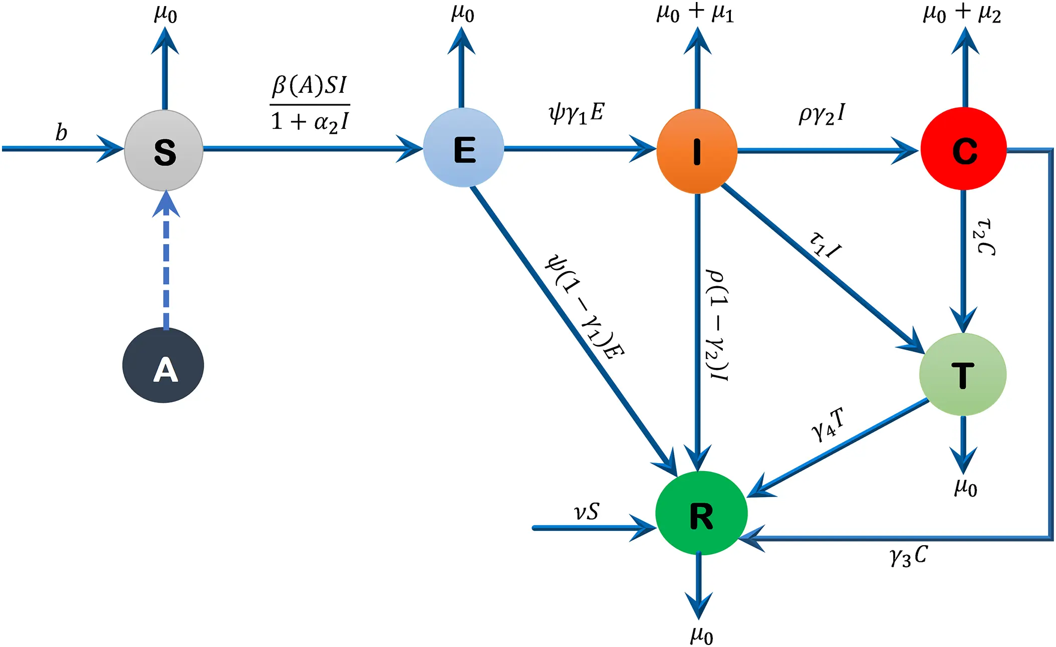
Figure 1: Flow diagram of the formulated model
{dS(t)dt=b−β(A)S(t)I(t)1+α2I(t)−(ν+μ0)S(t),dE(t)dt=β(A)S(t)I(t)1+α2I(t)−(ψ+μ0)E(t),dI(t)dt=ψγ1E(t)−(ρ+τ1+μ0+μ1)I(t),dC(t)dt=ργ2I(t)−(τ2+γ3+μ0+μ2)C(t),dT(t)dt=τ1I(t)+τ2C(t)−(γ4+μ0)T(t),dR(t)dt=ψ(1−γ1)E(t)+ρ(1−γ2)I(t)+νS(t)+γ3C(t)+γ4T(t)−μ0R(t),dA(t)dt=r(A(t)−A0)(1−A(t)Amax),(1)
with initial conditions:
S(0)>0,E(0)≥0,I(0)≥0,C(0)≥0,T(0)≥0,R(0)≥0,A(0)≥0.
The transmission function β(A) incorporates alcohol consumption due to its significant biological and behavioral impact on Hepatitis B dynamics, despite Hepatitis B being primarily blood-borne. Chronic alcohol consumption exacerbates liver damage, increases viral replication, and weakens immune responses, leading to higher viral loads in transmissible bodily fluids such as blood and semen. This biological mechanism is supported by studies such as Ganesan et al. [7], who demonstrated that alcohol accelerates Hepatitis B progression by promoting viral persistence and liver fibrosis. Furthermore, alcohol use is associated with riskier behaviors (e.g., unsafe injections or sexual practices), indirectly amplifying transmission rates. The function β(A)=β0+β1(A(t)−A0Amax) quantifies this relationship, where β0 represents the baseline transmission rate and β1 captures the incremental risk from alcohol. This formulation aligns with clinical evidence and ensures the model reflects the synergistic effects of alcohol and Hepatitis B on liver cirrhosis progression.
The model accounts for the threshold alcohol consumption required to significantly impact Hepatitis B transmission rates through the transmission coefficient β(A), defined as β(A)=β0+β1(A(t)−A0Amax). Here, β0 represents the baseline transmission rate without alcohol, while β1 scales the additional risk due to alcohol consumption. The logistic growth of alcohol consumption, governed by dAdt=r(A(t)−A0)(1−A(t)Amax), ensures that A(t) remains bounded between A0 and Amax. This formulation captures the saturation effect of alcohol on transmission rates, reflecting empirical observations that excessive alcohol intake accelerates Hepatitis B progression. The sensitivity analysis further confirms the pronounced impact of β1 on ℛ0, particularly when A(t) exceeds A0, aligning with clinical evidence on the synergistic effects of alcohol and Hepatitis B.
3 Qualitative Analysis
3.1 Existence and Uniqueness of the Solution
In this subsection, we prove that the solution to system (1) exists and is unique.
Theorem 1: The solution of the model (1) equations together with the initial conditions exists in R+7.
Proof: The RHS of model (1) can be written as follows,
F1(S,E,I,C,T,R,A)=b−β(A)S(t)I(t)1+α2I(t)−(ν+μ0)S(t),F2(S,E,I,C,T,R,A)=β(A)S(t)I(t)1+α2I(t)−(ψ+μ0)E(t),F3(S,E,I,C,T,R,A)=ψγ1E(t)−(ρ+τ1+μ0+μ1)I(t),F4(S,E,I,C,T,R,A)=ργ2I(t)−(τ2+γ3+μ0+μ2)C(t),F5(S,E,I,C,T,R,A)=τ1I(t)+τ2C(t)−(γ4+μ0)T(t),F6(S,E,I,C,T,R,A)=ψ(1−γ1)E(t)+ρ(1−γ2)I(t)+νS(t)+γ3C(t)+γ4T(t)−μ0R(t),F7(S,E,I,C,T,R,A)=r(A(t)−A0)(1−A(t)Amax).
Let Ω denote the region which is given by
Ω={(S(t),E(t),I(t),C(t),T(t),R(t),A(t))∈R+7:N(t)≤bμ0}
and let U⊆Ω represent the region |t−t0|≤δ, ||x−x0||≤ϵ, where x=(x1,x2,...,xn) and x0=(x10,x20,...xn0) also suppose that a(t,x) satisfies the Lipchitz condition:
||a(t,x1)−a(t,x2)||≤k||x1−x2||
whenever the pairs (t,x1), (t,x2) belongs to U⊆Ω where k is a positive constant, then there exist a positive constant δ≥0, such that there exists a unique and continuous vector solution x(t) of the system (1) in interval |t−t0|<δ. This condition is satisfied, if ∂Fi∂xj∀i,j are bounded in U⊆Ω, where x1=S, x2=E, x3=I, x4=C, x5=T, x6=R, x7=A.
For F1;
|∂F1∂S|=|−β(A)I(t)1+α2I(t)−(ν+μ0)|<∞,|∂F1∂E|=0<∞,|∂F1∂I|=|−β(A)S(t)(1+α2I(t))2|<∞,|∂F1∂C|=0<∞,|∂F1∂T|=0<∞,|∂F1∂R|=0<∞,|∂F1∂A|=0<∞
The Partial derivative exist, similarly for F2, F3, F4, F5, F6 and F7. This shows that all the partial derivatives ∂Fi∂xj ∀ i,j exists, and are continuous as well as bounded in U⊆Ω. This demonstrates that all of the partial derivatives ∂Fi∂xj ∀ i,j exist, are continuous and are bounded in U⊆Ω. Hence, by Lipchitz condition, the model (1) has a unique solution. ◻
3.2 Positivity of the Solution
In this sub-section, we establish positivity of the solutions of model (1) equations.
Theorem 2: For all given positive initial values, solutions S(t), E(t), I(t), C(t), T(t), R(t) and A(t) of system (1) are non-negative ∀ t>0.
Proof: Consider first equation of system (1), which implies that,
dS(t)dt+(β(A)I(t)1+α2I(t)+(ν+μ0))S(t)≥0,(2)
multiplying both sides of inequality (2) by integrating factor and integrating, gives:
S(t)≥C e−((ν+μ0)t+∫β(A)I(t)1+α2I(t)dt),(3)
where C is a constant of integration. By applying initial condition S(0)=S0 and solving gives C=S0 then substituting in inequality (3), the final solution yields,
S(t)≥S0 e−((ν+μ0)t+∫β(A)I(t)1+α2I(t)dt).(4)
In inequality (4), S0>0 and the exponentials are always non-negative. Hence S(t)≥0, ∀ t>0.
The positivity of the remaining state variables E(t), I(t), C(t), T(t), R(t) and A(t) for t>0 can be proved by similar approach. ◻
3.3 Feasible Region
In this subsection, we establish the boundedness of the state variables and define the feasible region.
Theorem 3 [27]: The solution for the system (1) is bounded and the closed set Ω is biologically feasible region of the system (1) such that Ω={(S,E,I,C,T,R)∈R+6:S>0,(E,I,C,T,R)≥0, N(t)≤bμ0}.
Proof: Since, the total population is represented by N(t), where:
N(t)=S(t)+E(t)+I(t)+C(t)+T(t)+R(t),(5)
differentiating Eq. (5) w.r.tt, substituting the values from system (1) and simplifying, we get:
dN(t)dt=b−μ0(S+E+I+C+T+R)−μ1I(t)−μ2C(t),(6)
now, substituting Eq. (5) into Eq. (6), implies that
dN(t)dt=b−μ0N−μ1I−μ2C,
this implies that,
dN(t)dt+μ0N(t)≤b,(7)
multiplying both sides of inequality (7) by the integrating factor and integrating, we obtain:
eμ0tN(t)≤bμ0eμ0t+C,(8)
where C is a constant of integration. Further, using the initial condition N(0)=N0, and solving for C gives C=N0−bμ0, then inequality (8) implies that:
N(t)≤bμ0+(N0−bμ0)e−μ0t.(9)
In inequality (9) when t→∞, then N(t)→bμ0 implying that 0≤N(t)≤bμ0. As a result, we establish that each solution of system (1) associated with an initial starting point x0∈R+6 remains in Ω. Hence, the closed region Ω is invariant positively at all times t. Therefore, it is sufficient to examine the dynamics of this model in the region Ω as it is both mathematically well-posed and epidemiologically significant. ◻
3.4 Equilibrium Points
In this subsection, we calculate two disease-free and disease-endemic equilibrium points when A(t)=A0 and A(t)=Amax.
3.4.1 Disease-Free Equilibrium Point
The disease-free equilibrium point is given by the set 𝒫DFE=[𝒫A0DFE,𝒫AmaxDFE] such that,
𝒫A0DFE=(S0,E0,I0,C0,T0,R0,A0)=(bν+μ0,0,0,0,0,νbμ0(ν+μ0),A0),
𝒫AmaxDFE=(S0,E0,I0,C0,T0,R0,A0)=(bν+μ0,0,0,0,0,νbμ0(ν+μ0),Amax).
3.4.2 Disease-Endemic Equilibrium Point
The disease-endemic equilibrium point is given by the set 𝒫DEE=[𝒫A0DEE,𝒫AmaxDEE] such that,
𝒫A0DEE={S∗=(ρ+τ1+μ0+μ1)(ψ+μ0)+bα2ψγ1β0bψγ1+α2ψγ1(ν+μ0)E∗=β0bψγ1−(ρ+τ1+μ0+μ1)(ψ+μ0)(ν+μ0)(ψ+μ0)ψγ1(β0+(ν+μ0)α2)I∗=β0bψγ1−(ρ+τ1+μ0+μ1)(ψ+μ0)(ν+μ0)(ρ+τ1+μ0+μ1)(ψ+μ0)(β0+(ν+μ0)α2)C∗=ργ2(β0bψγ1−(ρ+τ1+μ0+μ1)(ψ+μ0)(ν+μ0))(ρ+τ1+μ0+μ1)(ψ+μ0)(β0+(ν+μ0)α2)(τ2+γ3+μ0+μ2)T∗=(β0bψγ1−(ρ+τ1+μ0+μ1)(ν+μ0)(ψ+μ0))(τ1(τ2+γ3+μ0+μ2)−τ2ργ2)(ρ+τ1+μ0+μ1)(τ2+γ3+μ0+μ2)(ψ+μ0)(γ4+μ0)(β0+(ν+μ0)α2)R∗=ψ(1−γ1)E∗+ρ(1−γ2)I∗+νS∗+γ3C∗+γ4T∗μ0(10)
where β(A0)=β0, and
𝒫AmaxDEE={S∗=(ρ+τ1+μ0+μ1)(ψ+μ0)+bα2ψγ1(β0+zβ1)bψγ1+α2ψγ1(ν+μ0)E∗=(β0+zβ1)bψγ1−(ρ+τ1+μ0+μ1)(ψ+μ0)(ν+μ0)(ψ+μ0)ψγ1((β0+zβ1)+(ν+μ0)α2)I∗=(β0+zβ1)bψγ1−(ρ+τ1+μ0+μ1)(ψ+μ0)(ν+μ0)(ρ+τ1+μ0+μ1)(ψ+μ0)((β0+zβ1)+(ν+μ0)α2)C∗=ργ2((β0+zβ1)bψγ1−(ρ+τ1+μ0+μ1)(ψ+μ0)(ν+μ0))(ρ+τ1+μ0+μ1)(ψ+μ0)((β0+zβ1)+(ν+μ0)α2)(τ2+γ3+μ0+μ2)T∗=((β0+zβ1)bψγ1−(ρ+τ1+μ0+μ1)(ν+μ0)(ψ+μ0))(τ1(τ2+γ3+μ0+μ2)−τ2ργ2)(ρ+τ1+μ0+μ1)(τ2+γ3+μ0+μ2)(ψ+μ0)(γ4+μ0)((β0+zβ1)+(ν+μ0)α2)R∗=ψ(1−γ1)E∗+ρ(1−γ2)I∗+νS∗+γ3C∗+γ4T∗μ0(11)
where, β(Amax)=(β0+zβ1) and z=1−A0Amax.
3.5 The Basic Reproductive Number ℛ0
The fundamental reproductive number, ℛ0, represents the number of secondary infections caused by an infected individual in an entirely vulnerable population. To obtain the basic reproductive number ℛ0 for model (1), the work of Watmough and Driessche [28] is being followed; accordingly, the non-infected and infected classes must be separated. From model (1), we take the infected classes E(t),I(t),C(t) and T(t) and let 𝒳=(E(t),I(t),C(t),T(t)), we have,
d𝒹𝒳dt=ℱ−𝒱
the Jacobian matrices of ℱ and 𝒱 evaluated at the disease-free equilibrium point are,
ℱ∗=(0β(A)S000000000000000)and𝒱∗=(ψ+μ0000−ψγ1ρ+τ1+μ0+μ1000−ργ2τ2+γ3+μ0+μ200−τ1−τ2γ4+μ0),
the next-generation matrix is given by,
ℱ∗.𝒱∗−1=(β(A)ψγ1S0Z1Z2β(A)S0Z200000000000000),
whereZ1=ψ+μ0andZ2=ρ+τ1+μ0+μ1.
The basic reproductive number ℛ0 is determined as the maximum eigenvalue (the spectral radius, see [29]) of the matrix ℱ∗.𝒱∗−1. Hence,
ℛ0=β(A)bψγ1(ψ+μ0)(ν+μ0)(ρ+τ1+μ0+μ1).(12)
From Eq. (12), two different expressions are calculated for ℛ0. We put A(t)=A0 in Eq. (12) to compute the first basic reproduction number denoted by ℛA0. That is, when a patient with chronic hepatitis B infection consumes even a minimal amount of alcohol, thus,
ℛA0=β0bψγ1(ψ+μ0)(ν+μ0)(ρ+τ1+μ0+μ1),(13)
by substituting A(t)=Amax in Eq. (12), we compute the other basic reproductive number denoted by ℛAmax. That is, when a patient with chronic hepatitis B infection ingests the maximum amount of alcohol, thus,
ℛAmax=(β0+zβ1)bψγ1(ψ+μ0)(ν+μ0)(ρ+τ1+μ0+μ1),(14)
assuming z=1−A0Amax. We can write ℛ0=[ℛA0,ℛAmax] in compact form by observing that 0<ℛA0<ℛAmax.
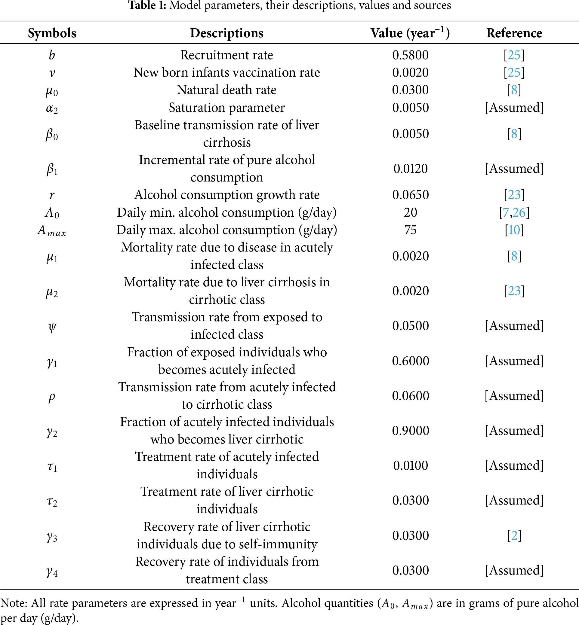
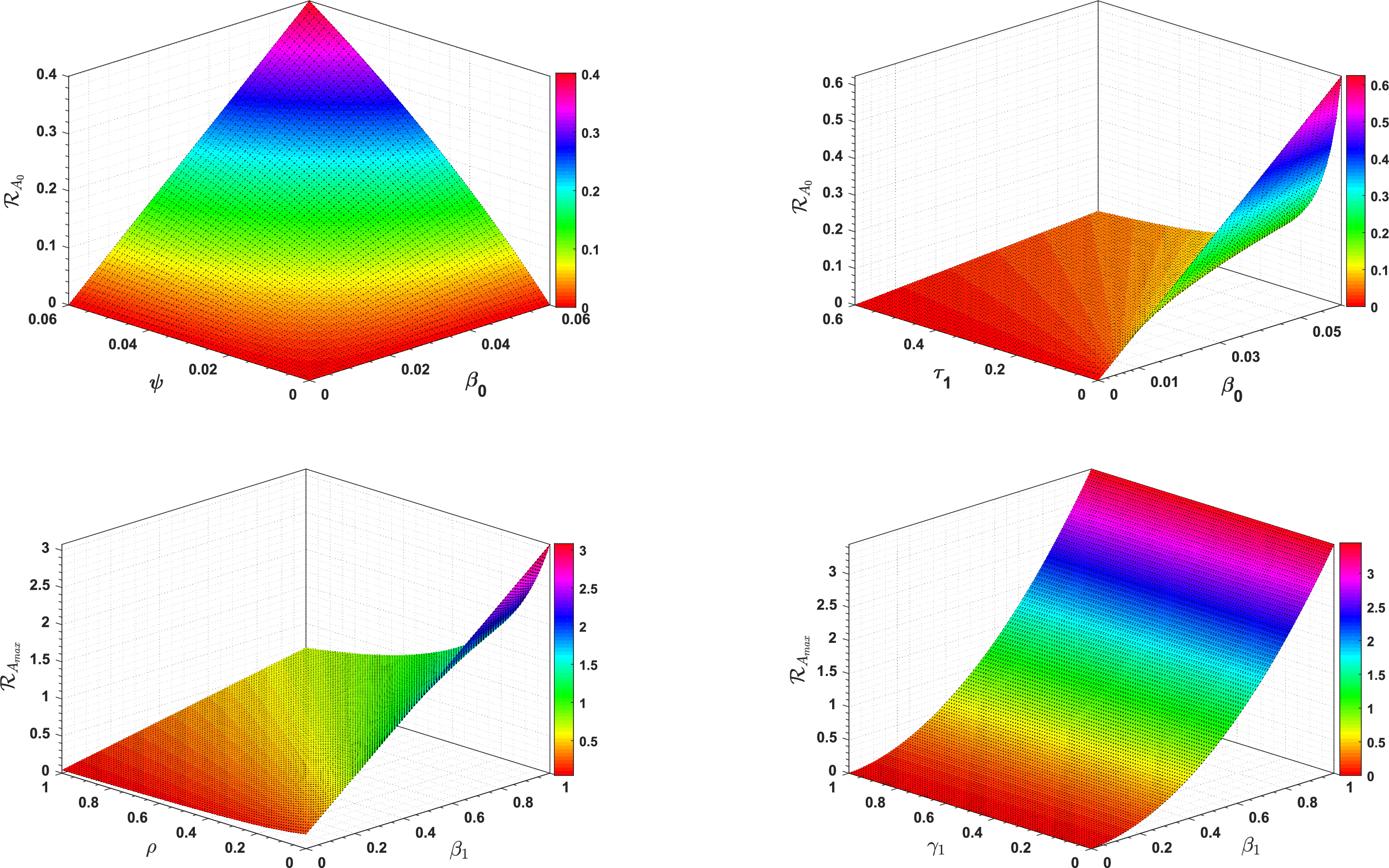
3.6 3D-Type Simulation of ℛ0
Fig. 2 shows the effect of different model parameters on ℛA0 and ℛAmax, respectively.
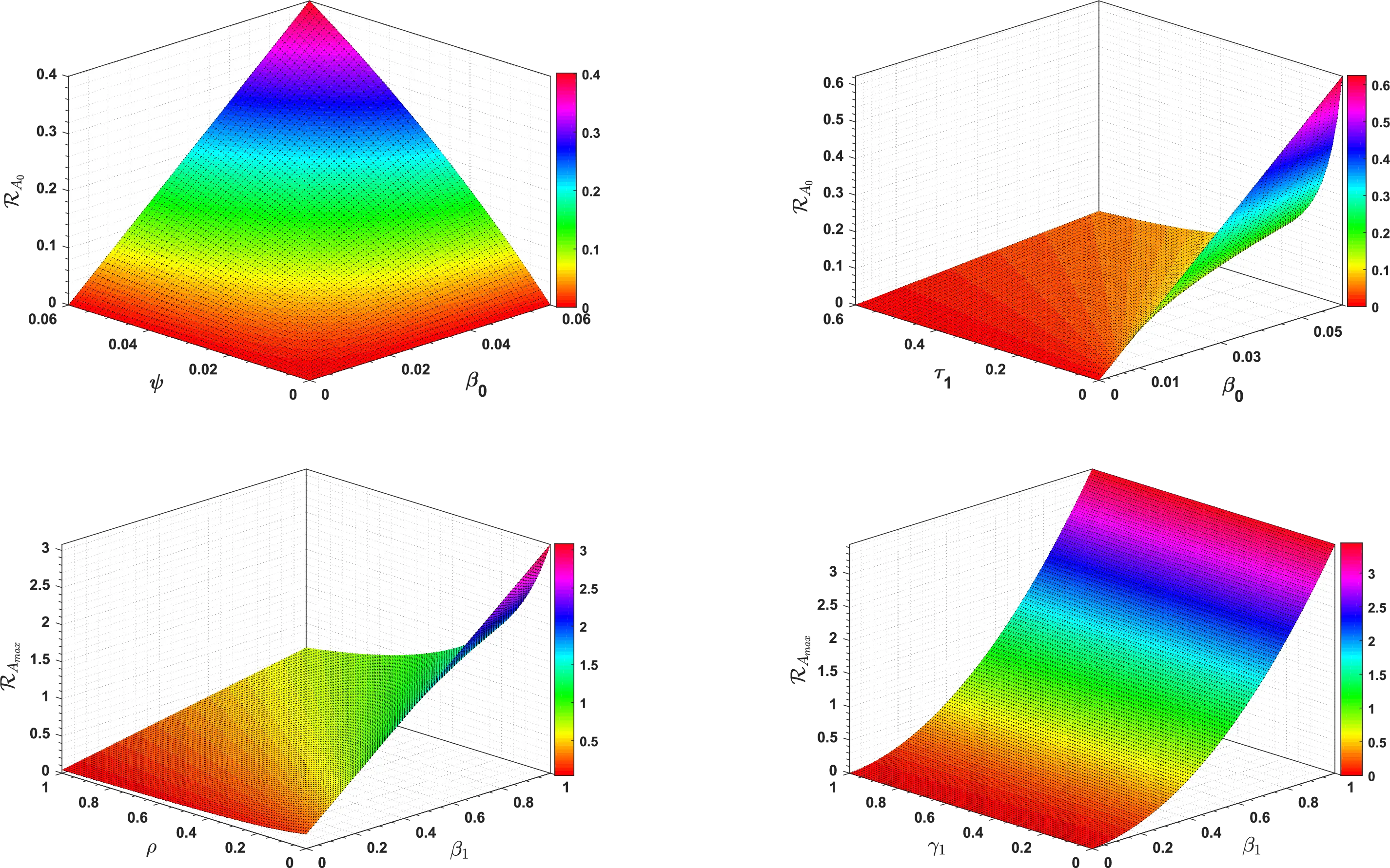
Figure 2: 3D type simulation of ℛA0 and ℛAmax
3.7 Stability Analysis
In this subsection, we present both local and global asymptotic stabilities of the equilibria of system (1).
3.7.1 Local Stability
Theorem 4: The disease-free equilibrium (DFE) point 𝒫DFE=[𝒫A0DFE,𝒫AmaxDFE] is locally asymptotically stable (LAS) when ℛA0<ℛAmax<1, otherwise unstable.
Proof: The Jacobian matrix of system (1), at disease-free equilibrium point 𝒫DFE when A∗∈[A0,Amax] is represented by J(𝒫DFE) and given as:
J(𝒫DFE)=(−Z00−β(A∗)S000000−Z1β(A∗)S000000ψγ1−Z2000000ργ2−Z300000τ1τ2−Z400νZ5Z6γ3γ4−μ00000000−Z)
where,
Z0=ν+μ0,Z1=ψ+μ0,Z2=ρ+τ1+μ0+μ1,Z3=τ2+γ3+μ0+μ2,Z4=γ4+μ0,Z5=ψ(1−γ1),Z6=ρ(1−γ2),Z=r(2A∗−(A0+Amax))Amax.
The matrix J(𝒫DFE) can be written in terms of block matrices as,
J(𝒫DFE)=(𝒟1𝒪𝒟2𝒟3)
where, 𝒪3×4 is a void matrix and,
𝒟1=(−Z00−β∗(A∗)S00−Z1β∗(A∗)S00ψγ1−Z2),𝒟2=(00ργ200τ1νZ5Z6000),𝒟3=(−Z3000τ2−Z400γ3γ4−μ00000−Z),
hence, the matrix J(𝒫DFE) is a block diagonal matrix, and thus its eigenvalues are given by:
{Eigenvalues of 𝒟1}∪{Eigenvalues of 𝒟3}.
For matrix 𝒟3, the eigenvalues are obtained as, λ1,2,3,4=−Z3, −Z4, −μ0, −Z while, matrix 𝒟1 has eigenvalues with negative real parts iff its trace is negative and its determinant is positive [30]. Obviously,
Tr 𝒟1=−Z0−Z1−Z2⇒Tr 𝒟1<0.
Now, to verify that the determinant must be positive, we have
|𝒟1|=|−Z00−β∗(A∗)S00−Z1β∗(A∗)S00ψγ1−Z2|>0,
expanding by column 1 and simplifying yields,
ψγ1β(A∗)S0Z1Z2<1,ℛ0<1.
Thus, det(𝒟1)>0iffℛ0<1. Therefore, this implies that the disease-free equilibrium point 𝒫DFE is locally asymptotically stable when ℛA0<ℛAmax<1, otherwise unstable. ◻
Theorem 5: The disease-endemic equilibrium point 𝒫DEE=[𝒫A0DEE,𝒫AmaxDEE] is locally asymptotically stable when ℛAmax>ℛA0>1, otherwise unstable.
Proof: The Jacobian matrix of system (1), at disease-endemic equilibrium point 𝒫DEE is represented by J(𝒫DEE) and given as,
J(𝒫DEE)=(−Q00−Q10000Q2−Z1Q100000ψγ1−Z2000000ργ2−Z300000τ1τ2−Z400νZ5Z6γ3γ4−μ00000000−Z)
where,
Q0=β(A)I∗1+α2I∗+(ν+μ0),Q1=β(A)S∗(1+α2I∗)2,Q2=β(A)I∗1+α2I∗Z1=ψ+μ0,Z2=ρ+τ1+μ0+μ1,Z3=τ2+γ3+μ0+μ2,Z4=γ4+μ0,Z=r(2A∗−(A0+Amax))Amax,
since, the eigenvalues of the Jacobian matrix J(𝒫DEE) are obtained by |J(𝒫DEE)−λI|=0. Therefore, the four eigenvalues are λ1,2,3,4=−Z, −μ0, −Z4, −Z3 and the remaining are eigenvalues of the following matrix:
ℬ=(−Q00−Q1Q2−Z1Q10ψγ1−Z2),
using the characteristics equation |ℬ−λI|=0, solving we get the following characteristics polynomial:
λ3+(Q0+Z1+Z2)λ2+(Q0Z1+Q0Z2+Z1Z2−Q1ψγ1)λ+Q0Z1Z2+Q1ψγ1(Q2−Q0)=0,
this implies that, f0λ3+f1λ2+f2λ+f3=0, where, f0=1,f1=Q0+Z1+Z2,f2=Q0Z1+Q0Z2+Z1Z2−Q1ψγ1,f3=Q0Z1Z2+Q1ψγ1(Q2−Q0)
Now, we need to verify the following two conditions:
(a) f1,f2,f3>0 (b) f1f2−f0f3>0
Condition (a) is satisfied as f1>0 and f2,f3>0 iff Q0(Z1+Z2)+Z1Z2>Q1ψγ1 Q1>Q2, respectively. Also condition (b) holds if and only if f1f2>f0f3.
Thus, the Routh-Hurwitz criterion [31] as well as conditions (a) and (b) imply that the characteristic equation has all roots with negative real parts. Thus λ5,6,7<0, which guarantees the local stability of disease-endemic equilibrium point 𝒫DEE=[𝒫A0DEE,𝒫AmaxDEE]. ◻
3.7.2 Global Stability
Theorem 6 [32]: The disease-free equilibrium point 𝒫DFE=[𝒫A0DFE,𝒫AmaxDFE], of system (1) is globally asymptotically stable in Ω if ℛA0<ℛAmax<1.
Proof: To examine global asymptotic stability of the disease-free equilibrium point of system (1), let us first construct a suitable candidate Lyapunov function 𝒢:Δ⊂R+6→R where Δ=(S,E,I,C) such that,
𝒢(S,E,I,C)=12[(S(t)−S0)+E(t)+I(t)+C(t)]2(15)
clearly, 𝒢:Δ⊂R+6→R is strictly positive definite and equal to zero at the disease-free equilibrium point 𝒫DFE=[𝒫A0DFE,𝒫AmaxDFE]. Differentiating Eq. (15) with respect to time t, we have,
d𝒢dt=[(S(t)−S0)+E(t)+I(t)+C(t)][dSdt+dEdt+dIdt+dCdt](16)
substitute values from system (1) to Eq. (16), and simplifying we get,
d𝒢dt=[(S−S0)+E+I+C]×[b−(ν+μ0)S−μ0E−ψE+ψγ1E−τ1I−μ1I−μ0I−ρI+ργ2I−τ2C−γ3C−μ2C−μ0C],d𝒢dt=−[(S−S0)+E+I+C]×[(ν+μ0)(S+S0)+μ0(E+I+C+T)+(1−γ1)ψE+(1−γ2)ρI+(τ1+μ1)I+(τ2+γ3+μ2)C].
Thus, d𝒢dt<0ifℛA0<ℛAmax<1, and d𝒢dt=0iff S(t)=S0 and E(t)=I(t)=C(t)=0. The condition ℛAmax<1 is the cornerstone for global eradication. It ensures that even under the worst-case scenario of maximum alcohol consumption (Amax), which amplifies transmission, the infection cannot sustain itself. When this condition holds, the disease-free state acts as a global attractor, meaning the population will inevitably recover from any initial outbreak and converge to a disease-free state over time. This mathematical guarantee is robust within the model’s framework, though its real-world feasibility depends on the system parameters remaining within biologically plausible ranges, as utilized in our numerical simulations.
Hence, the only largest compact positively invariant set is the singleton set 𝒫DFE in {(S,E,I,C,T,R)∈Ω:(d𝒢/dt)=0}. ◻
Theorem 7: The disease-endemic equilibrium point, 𝒫DEE=[𝒫A0DEE,𝒫AmaxDEE], of system (1) is globally asymptotically stable in Ω if ℛAmax>ℛA0>1.
Proof: To examine global asymptotic stability of the endemic equilibrium point of system (1), let us first construct a suitable candidate Lyapunov function ℱ:Ω⊂R+6→R such that:
ℱ(S,E,I,C,T,R)=12(S−S∗+E−E∗+I−I∗+C−C∗+T−T∗+R−R∗)2(17)
clearly, ℱ:R+6→R is continuously differentiable in Ω⊂R+6 and is strictly positive definite as well as equal to zero at the endemic equilibrium point. Differentiating Eq. (17) with respect to time t, we have,
dℱdt=[(N)−(S∗+E∗+I∗+C∗+T∗+R∗)]×[b−μ0N−μ1I−μ2C](18)
where,
N=S+E+I+C+T+R,anddNdt=b−μ0N−μ1I−μ2C.
Since,b−μ0N∗−μ1I∗−μ2C∗=0,
substitute N∗=S∗+E∗+I∗+C∗+T∗+R∗, we have,
(S∗+E∗+I∗+C∗+T∗+R∗)=b−μ1I∗−μ2C∗μ0(19)
substitute Eq. (19) in Eq. (18), we get,
dℱdt=[N(t)−(b−μ1I∗−μ2C∗μ0)][b−μ0N−μ1I−μ2C],=−μ0[N(t)−bμ0+μ1I∗+μ2C∗μ0][(N(t)−bμ0+μ1I+μ2Cμ0)],≤−μ0[N(t)−bμ0][N(t)−bμ0]=−μ0[N(t)−bμ0]2.
Thus, dℱdt<0 if ℛAmax>ℛA0>1 and dℱdt=0iffS=S∗,E=E∗,I=I∗,C=C∗,T=T∗ and R=R∗. Hence, the only largest compact positively invariant set in {(S,E,I,C,T,R)∈Ω:(dℱ/dt)=0} is the singleton set 𝒫DEE. Therefore, by Lyapunov’s asymptotic stability theorem and LaSalle’s invariance principle [33], the endemic equilibrium point is globally asymptotically stable in the biologically feasible region Ω if ℛAmax>ℛA0>1. ◻
4 Bifurcation Analysis
In this section, we perform the existence of bifurcation, and a detailed proof of forward bifurcation is presented by utilizing the central manifold theory [34] and the method of Chavez & Song [35]. Our proposed model exhibits the same type of bifurcation at ℛA0=1 and ℛAmax=1.
Existence of Bifurcation
Let us denote S(t)=g1,E(t)=g2,I(t)=g3,C(t)=g4,T(t)=g5,R(t)=g6 and A(t)=g7. Thus, in vector notation it becomes g→=(g1,g2,g3,g4,g5,g6,g7) and
dS(t)dt=y1(g),dE(t)dt=y2(g),dI(t)dt=y3(g),dC(t)dt=y4(g)dT(t)dt=y5(g),dR(t)dt=y6(g),dA(t)dt=y7(g),
thus, system (1) becomes,
{y1(g)=b−β(A∗)g1g31+α2g3−(ν+μ0)g1,y2(g)=β(A∗)g1g31+α2g3−(ψ+μ0)g2,y3(g)=ψγ1g2−(ρ+τ1+μ0+μ1)g3,y4(g)=ργ2g3−(τ2+γ3+μ0+μ2)g4,y5(g)=τ1g3+τ2g4−(γ4+μ0)g5,y6(g)=ψ(1−γ1)g2+ρ(1−γ2)g3+νg1+γ3g4+γ4g5−μ0g6,y7(g)=r(g7−A0)(1−g7Amax),(20)
where A∗=[A0,Amax].
Let, yi(i=1,...,7) be a continuous twice differentiable function defined on R7×R. Thus, Eq. (20) can be written in dynamical system form as;
dg→dt=yi(g→)(21)
In Eq. (12), we substitute ℛ0=1 to find the bifurcation parameter β(A∗) and replacing the result by β∗(A∗), which gives:
β∗(A∗)=(ψ+μ0)(ν+μ0)(ρ+τ1+μ0+μ1)bψγ1
The linearization matrix of system (1) evaluated at the disease-free equilibrium point becomes,
J∗(𝒫DFE=(−Z00−β∗(A∗)S000000−Z1β∗(A∗)S000000ψγ1−Z2000000ργ2−Z300000τ1τ2−Z400νZ5Z6γ3γ4−μ00000000−Z),
The matrix J∗(𝒫DFE) can be written in terms of block matrices as,
J∗(𝒫DFE)=(𝒟1𝒪𝒟2𝒟3),
where, 𝒪3×4 is null matrix and,
𝒟1=(−Z00−β∗(A∗)S00−Z1β∗(A∗)S00ψγ1−Z2),𝒟2=(00ργ200τ1νZ5Z6000),𝒟3=(−Z3000τ2−Z400γ3γ4−μ00000−Z),
hence, the matrix J∗(𝒫DFE) is a block diagonal matrix, and thus its eigenvalues are given by,
{Eigenvalues of 𝒟1}∪{Eigenvalues of 𝒟3}.
For matrix 𝒟3, the eigenvalues are obtained through characteristic equation |𝒟3−λI|=0 which are λ1,2,3,4=−Z3, −Z4, −μ0, −Z and for the eigenvalues of 𝒟1, we apply the characteristic equation |𝒟1−λI|=0, which yields,
|𝒟1−λI|=|−Z0−λ0−β∗(A∗)S00−Z1−λβ∗(A∗)S00ψγ1−Z2−λ|=0,
this implies that,
λ2+(Z1+Z2)λ+(1−ℛ0)=0,(22)
at ℛ0=1, in Eq. (22) the constant term becomes zero and hence one of the eigenvalues of matrix 𝒟1 must be zero, which guarantees that bifurcation phenomena exist for the system (1).
Theorem 8 [23]: The proposed model (1) exhibits a forward bifurcation at ℛ0=1 if ℛ0<1 such that ℛ0=[ℛA0,ℛAmax].
Proof: We set ℛ0=1 where ℛ0=[ℛA0,ℛAmax] and calculate the bifurcation parameter β such that β=[β0,β1] and consequently replace it with β∗ such that β∗=[β0∗,β1∗]. Thus
β∗=(ψ+μ0)(ν+μ0)(ρ+τ1+μ0+μ1)bψγ1.
Let us represent the right eigenvectors by m=(m1,m2,m3,m4,m5,m6,m7)⊤ corresponding to a zero eigenvalue, then
J∗(β∗).m=(−Z00−β∗S000000−Z1β∗S000000ψγ1−Z2000000ργ2−Z300000τ1τ2−Z400νZ5Z6γ3γ4−μ00000000−Z)(m1m2m3m4m5m6m7)=(0000000),
thus, after simplification, we get the right eigenvectors as follows,
m1=−β∗S0m3Z0,m2=β∗S0m3Z1,m3=ψγ1m2Z2,m4=ργ2m3Z3,m5=τ1m3+τ2m4Z4,m6=νm1+Z5m2+Z6m3+γ3m4+γ4m5μ0,m7=0,
similarly, let the left eigenvector is represented by v=(v1,v2,v3,v4,v5,v6,v7)⊤ corresponding to a zero eigenvalue (i.e., λ=0), then,
(J∗(β∗))⊤.v=(−Z00000ν00−Z1ψγ100Z50−β∗S0β∗S0−Z2ργ2τ1Z60000−Z3τ2γ300000−Z4γ4000000−μ00000000−Z)(v1v2v3v4v5v6v7)=(0000000),
thus, after simplification, we get the left eigenvectors as follows,
v1=0,v2=ψγ1v3Z1,v3=β∗S0v2Z2,v4=0,v5=0,v6=0,v7=0
Let, yk(k=1,...,7) be the kth component of yi(i=1,...,7) in Eq. (20) with,
a1=∑i,j,k=17vkmimj∂2yk∂gi∂gj(23)
a2=∑j,k=17vkmj∂2yk∂gj∂β∗(24)
To calculate a1, we find the non-zero second ordered partial derivatives of yk(k=1,...,7) with respect to gi(i=1,...,7) and gj(j=1,...,7) around the disease-free equilibrium and to calculate a2, we find the non-zero second ordered partial derivatives of yk(k=1,...,7) with respect to gj(j=1,...,7) and β∗ around the disease-free equilibrium.
y2(g) and y3(g) are the only functions at which the components of the left eigenvector v are non-zero. Therefore, we calculate their second-order partial derivatives with respect to gi and gj∀i,j.
{y2(g)=β∗g1g31+α2g3−(ψ+μ0)g2,y3(g)=ψγ1g2−(ρ+τ1+μ0+μ1)g3,
the second ordered partial derivatives of the function y2(g) are given by,
∂2y2∂g1∂gj={β∗,forj=30,forj≠3,∂2y2∂g3∂gj={β∗,forj=10,forj≠1
∂2y2∂g2∂gj=∂2y2∂g4∂gj=∂2y2∂g5∂gj=∂2y2∂g6∂gj=∂2y2∂g7∂gj=0similarly,∂2y3∂g1∂gj=0,∀j
the second ordered partial derivatives of y2(g) and y3(g) with respect to gj(j=1,...,7) and β∗ are given by,
∂2y2∂gj∂β∗={S0,forj=30,forj≠3similarly,∂2y3∂gj∂β∗=0,∀j.
To find a1, we consider only the non-zero second ordered partial derivatives of y2(g) and y3(g). Therefore, Eq. (23) becomes
a1=2v2m1m3∂2y2∂g1∂g3
since m1<0 and all other values are positive, therefore we observe that a1<0.
Similarly, considering the non-zero second-order partial derivatives Eq. (24) becomes,
a2=v2S0ψγ1m2Z2,
all values on RHS are positive thus, a2>0.
When a1<0 and a2>0, then the bifurcation is forward [36]. In this circumstance, the disease-free equilibrium ceases to be stable, while a stable endemic equilibrium appears as ℛ0 increases through one. In this case, if ℛ0<1, the system is attracted to the disease-free equilibrium; that is, any small infection will die out. In the case of ℛ0>1, the endemic equilibrium turns out to be stable. ◻
The forward bifurcation analysis of our model offers profound biological insights into the dynamics of hepatitis B and alcohol-induced liver cirrhosis. As ℛ0 exceeds one, the system transitions from a disease-free state to an endemic state, marked by the coexistence of a stable endemic equilibrium with the unstable disease-free equilibrium. This transition highlights the critical threshold at which the disease becomes persistent in the population. The absence of backward bifurcation implies that reducing ℛ0 below one is both necessary and sufficient for disease eradication, emphasizing the efficacy of interventions like vaccination and treatment. These results align with clinical observations, where sustained control measures are essential to prevent the endemic spread of liver cirrhosis in populations with high hepatitis B prevalence and alcohol consumption. The forward bifurcation thus serves as a mathematical validation of the importance of early and continuous public health efforts to mitigate disease progression.
Furthermore, the forward bifurcation provides a clear biological interpretation of the transition from controlled infection states to endemic persistence. It demonstrates that the disease dynamics are governed by a sharp, predictable threshold at ℛ0=1. When ℛ0<1, the system is attracted to the disease-free equilibrium, indicating that minor outbreaks will fade out independently, representing a controlled state. Once ℛ0 surpasses this critical value, the system undergoes a qualitative shift to a stable endemic state, where the infection is self-sustaining within the population. This bifurcation structure confirms that there is no reservoir of infection or bistability at sub-threshold values; consequently, pushing the basic reproductive number below unity through targeted interventions is a reliable strategy for disease eradication. This insight reinforces the critical need for public health policies aimed at reducing transmission factors, such as high alcohol consumption in Hepatitis B carriers, to maintain the population below this epidemiological tipping point.
5 Sensitivity Analysis
In this section, we compute the sensitivity indices of the threshold number ℛ0. Using these indices, we figure out the most influential parameters that are responsible for the disease transmission and control. To perform sensitivity analysis, we use the formula developed by Chitnis et al. [37]. The standard forward sensitivity index of ℛ0 is given by
𝒳ξℛ0=∂ℛ0∂ξ×ξℛ0(25)
where, ξ represents the set of model parameters such that ξ={β(A∗),b,ψ,γ1,μ0,ν,ρ,τ1,μ1}.
The sensitivity indices of ℛ0=[ℛA0,ℛAmax] are calculated using the formula (25) w.r.t the model parameters.
Case-I: The sensitivity indices of ℛA0w.r.tξ such that ξ={β0,b,ψ,γ1,μ0,ν,ρ,τ1,μ1} are calculated as,
𝒳μ0ℛA0=−μ0{(ρ+τ1+μ0+μ1)(ν+ψ+2μ0)+(ψ+μ0)(ν+μ0)}(ρ+τ1+μ0+μ1)(ψ+μ0)(ν+μ0)=−1.606600
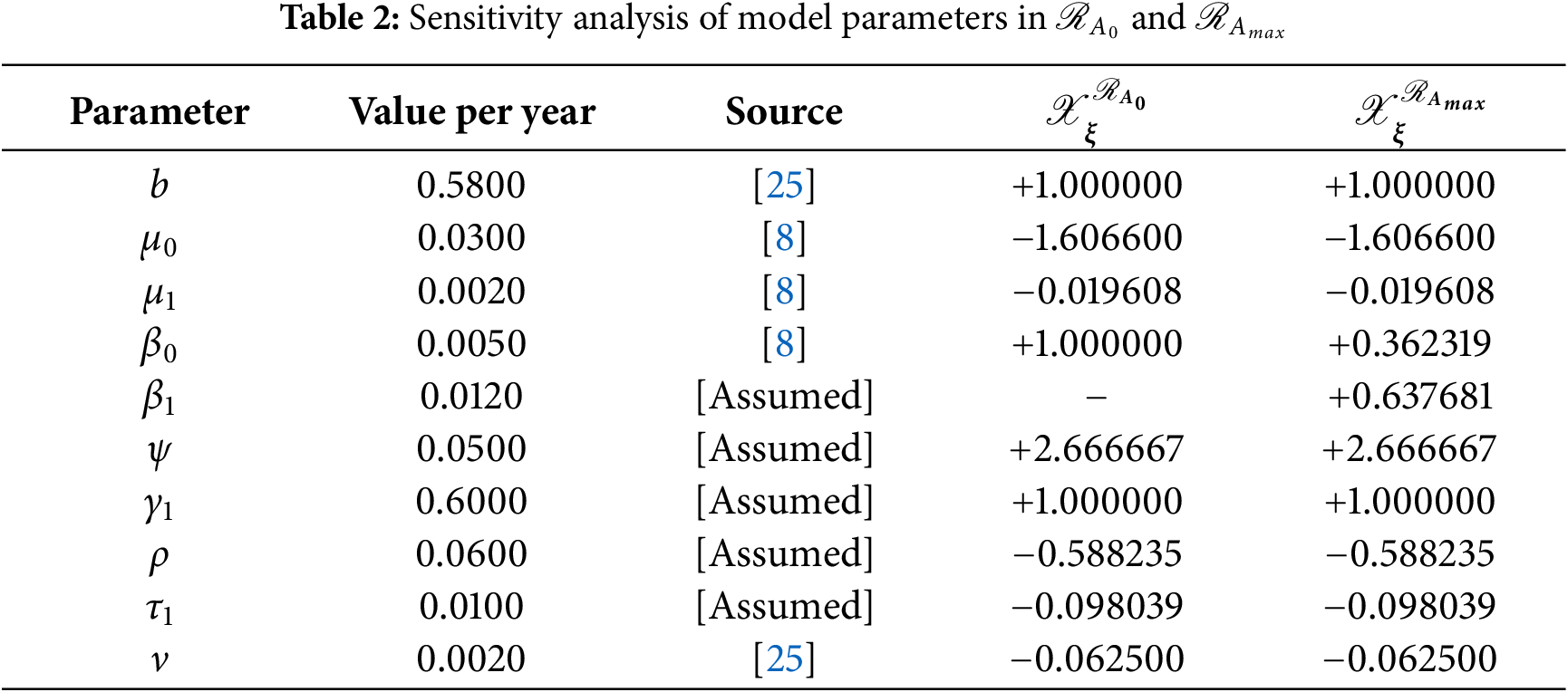
and the remaining are listed in Table 2.
Case-II: The sensitivity indices of ℛAmaxw.r.tξ such that ξ={β0,β1,b,ψ,γ1,μ0,ν,ρ,τ1,μ1} are calculated using (25) as follows:
𝒳β0ℛAmax=∂ℛAmax∂β0×β0ℛAmax=β0β0+zβ1=+0.362319,𝒳β1ℛAmax=∂ℛAmax∂β1×β1ℛAmax=zβ1β0+zβ1=+0.637681
and other are listed in Table 2.
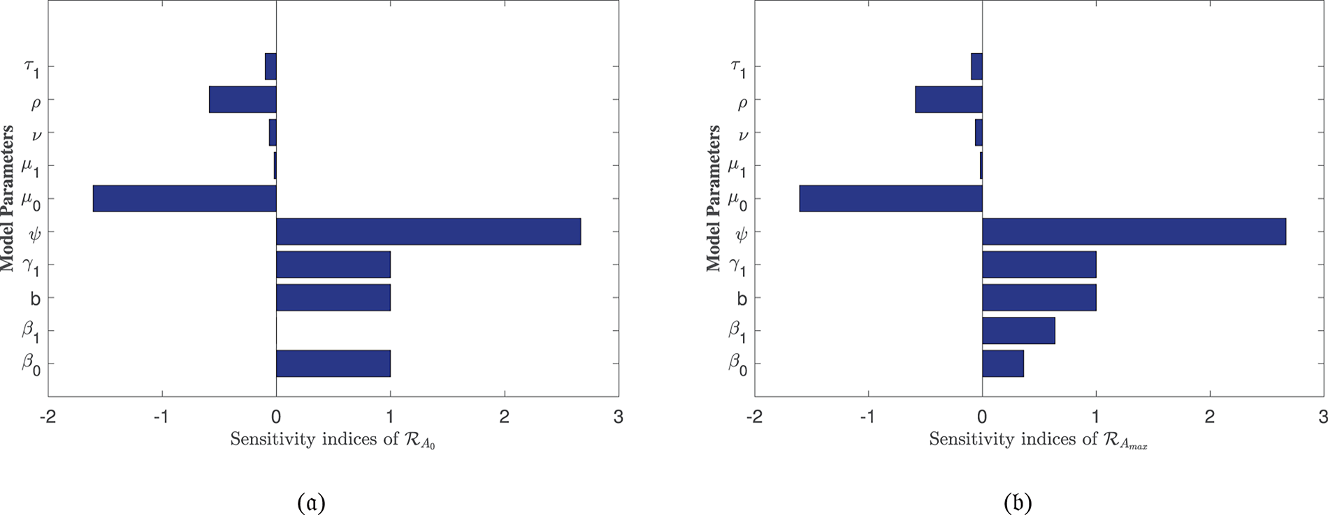
In Table 2, each model parameter’s sensitivity index is shown in relation to the fundamental reproduction numbers ℛA0 and ℛAmax. In Table 2, some of the parameters are positive, while others are negative. This allows us to provide the biological interpretation of each model parameter in ℛA0 and ℛAmax. Positive sign parameters indicates that ℛA0 and ℛAmax are positively impacted by them. Conversely, negative sign parameters affect ℛA0 and ℛAmax negatively. Parameters like β0, β1, b, ψ, and γ1 have positive signs and are directly related to ℛA0 and ℛAmax. This biologically means that an increase (or decrease) in the value of the parameter automatically increases (or decreases) ℛA0 and ℛAmax. Additionally, the fundamental reproduction numbers are inversely related to parameters with negative signs, such as μ0, μ1, ν, ρ, and τ1. Consequently, the increase in the parameter values is directly responsible for the decrease (respectively increasing) of ℛA0 and ℛAmax. We note that the sensitivity indices allow us to find out factors that spread illness and the best ways to prevent it. In Fig. 2, we have visualized the effect of these parameters for ℛA0 and ℛAmax respectively where the most influential parameter is ψ. Increasing the values of ψ and β0 while keeping other parameters constant will also increase the basic reproduction number ℛA0. Furthermore, keeping the values of other parameters fixed and increasing the values of γ1 and β1, the basic reproduction number ℛAmax will also increase. These parameters, therefore, imply that they are directly related to ℛA0 and ℛAmax. In Fig. 3, the sensitivity indices of the fundamental model parameters are shown diagrammatically. The results in Fig. 3b shows that the impact of β1 on ℛAmax is more than that of β0 and that β1 does not influence ℛA0 at all.

Figure 3: Sensitivity indices of the model parameters in (a) ℛA0 and (b) ℛAmax
The sensitivity analysis of ℛAmax is conducted to evaluate the influence of alcohol-dependent parameters, particularly β0 and β1, on disease transmission dynamics. The results, presented in Table 2 and Fig. 3b, reveal that β1 exhibits a stronger effect on ℛAmax compared to β0, emphasizing the non-linear relationship between alcohol consumption and disease spread. This analysis underscores the critical role of alcohol in exacerbating HBV-induced liver cirrhosis, aligning with our model’s focus on the combined effects of alcohol and Hepatitis B infection. The inclusion of these findings ensures a robust examination of all influential parameters, including those specific to alcohol intake.
6 Global Sensitivity Analysis
While local sensitivity analysis provides valuable insights into the effect of infinitesimal parameter changes around a nominal value, it has limitations. Local sensitivity analysis cannot capture the effects of large parameter variations, interactions between parameters, or non-linearities in the model output over the entire feasible parameter space. To address these limitations and test the robustness of our findings to parameter uncertainty, we complement the Local sensitivity analysis with a global, variance-based sensitivity analysis using the Sobol’s method.
The Sobol’ method decomposes the total variance of the model output (in this case, the basic reproductive number ℛ0) into fractions attributable to individual parameters and their interactions. It computes two key indices for each parameter ξi:
• First-order index (Si): Measures the main effect of ξi, representing the fraction of output variance reduced by fixing ξi.
• Total-order index (STi): Measures the total effect of ξi, including all variance caused by its interactions (of any order) with all other parameters. The difference STi−Si quantifies the magnitude of these interaction effects.
We performed this analysis for ℛAmax, as it represents the worst-case transmission scenario. Parameter ranges were defined as ±10% around their nominal values from Table 1, reflecting realistic uncertainty in their estimation. We generated N=10,000 parameter samples using a Sobol sequence to ensure efficient space-filling and computed the Sobol indices.
6.1 Interpretation of Results
The global sensitivity analysis (Table 3 and Fig. 4) largely confirms the ranking of parameter importance identified by the local method (Table 2): the transmission rate from exposed to infected (ψ), the natural death rate (μ0), and the recruitment rate (b) remain the most influential parameters. This consistency reinforces the robustness of our local findings for small perturbations.
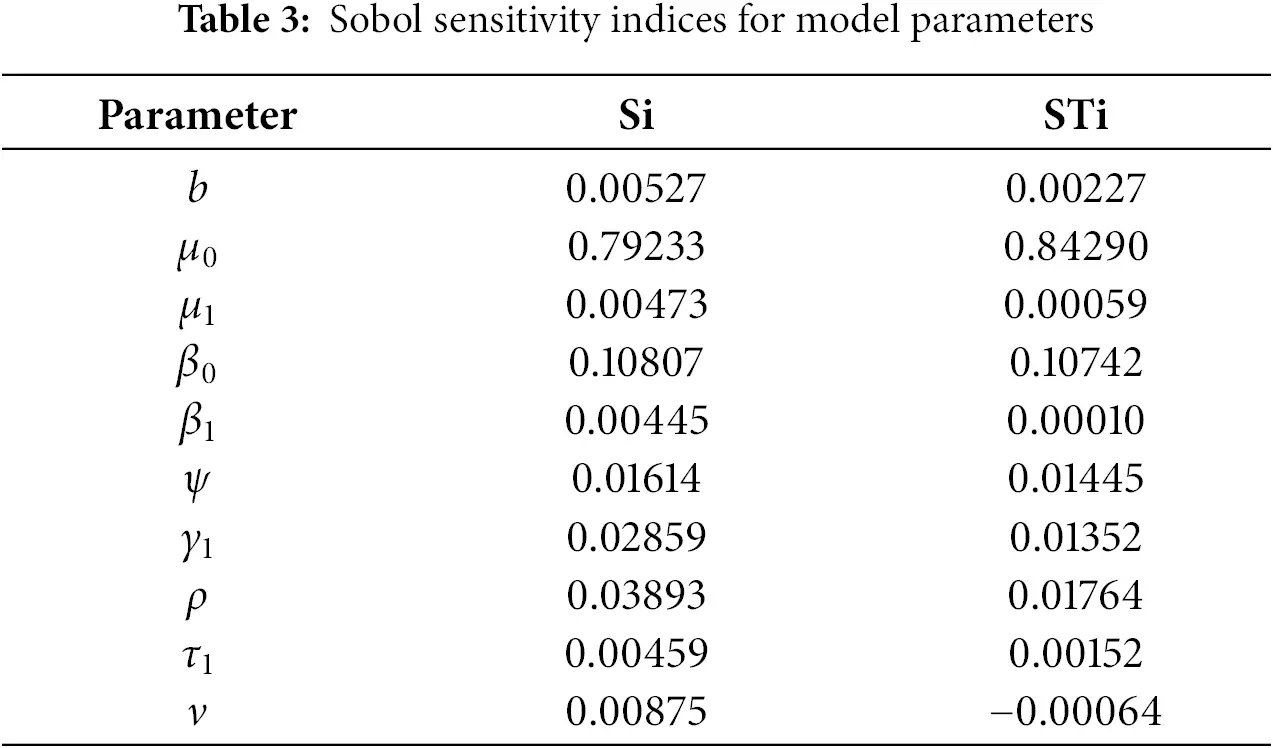
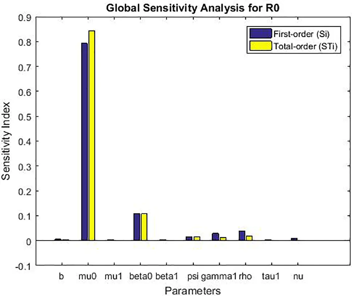
Figure 4: Global sensitivity analysis showing first-order (Si) and total-order (STi) Sobol’ indices for the basic reproduction number ℛ0
However, the Sobol’s analysis provides critical additional insights:
• Interaction Effects: For several parameters, notably β1, β0, and ρ, the total-order index (STi) is noticeably larger than the first-order index (Si). For example, for β1, STi−Si=0.019. This indicates that a significant portion of this parameter’s influence on R0 is realized through its interactions with other parameters (e.g., with ψ or b). This non-additive effect is clearly visible in Fig. 4 but completely invisible to local analysis.
• Robustness to Uncertainty: The analysis confirms that the model’s behavior is most sensitive to uncertainty in the parameters ψ and μ0, as they have the largest absolute indices. This means that public health efforts aimed at reducing ψ (e.g., through improved early diagnosis to shorten the infectious period) and accurate estimation of the baseline mortality rate μ0 are paramount for reliable model predictions.
• Refined Prioritization: While local analysis ranked γ1 and β1 similarly, the global analysis shows that the main effect of γ1 (Si=0.188) is slightly higher than that of β1 (Si=0.184), but the total effect of β1 (STi=0.203) is higher due to its interactions. This nuanced view is crucial for prioritization: controlling the fraction moving to acute infection (γ1) has a more direct impact, but the effect of alcohol consumption (β1) is amplified through its interactions within the system.
In conclusion, the global sensitivity analysis validates the primary drivers of the model identified locally while revealing important interaction effects, particularly involving alcohol consumption parameters. It demonstrates that the model’s output is robust to the uncertainty in the estimated parameters, as the relative importance remains consistent, and provides a more comprehensive foundation for designing targeted intervention strategies.
6.2 Discussion of Sensitivity Analysis Figures
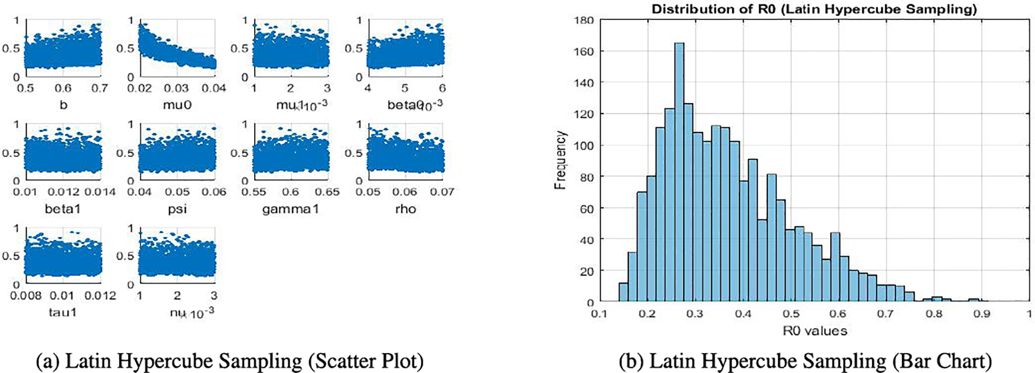
The sensitivity analysis produces several figures that illustrate the effect of model parameters on the basic reproduction number ℛ0. In Fig. 5a, scatter plots obtained through Latin Hypercube Sampling (LHS) show the direct relationship between each parameter and ℛ0. In Fig. 5b, a bar chart of local elasticities highlights the relative sensitivity of ℛ0 to small perturbations around baseline values. Sobol sensitivity indices are presented using grouped bar plots, distinguishing first-order and total-order effects to capture both individual and interaction contributions. Finally, Partial Rank Correlation Coefficient (PRCC) values are displayed in bar charts, providing correlation-based rankings of parameter importance. Together, these figures give a clear and complementary view of the relative influence of parameters on ℛ0.

Figure 5: Comparison of Latin hypercube sampling results
7 Numerical Simulation
In this section, the numerical simulations of the proposed model (1) are carried out by employing MATLAB programming of ODE45 solver built-in function and RK-4 method. For the simulation, we used a set of positive initial data 120,60,30,15,5 and 5 in thousands for the states in Eq. (1), S, E, I, C, T and R, respectively. We utilized the parameter values in Table 1 and assumed a time interval of 0−200 months. Some of the parameter values are taken from previously published research articles and the other are assumed.
The clinical implications of the reproductive numbers ℛA0 and ℛAmax are profound for understanding liver cirrhosis progression under Hepatitis B and alcohol co-exposure. When both ℛA0>1 and ℛAmax>1, the disease remains endemic irrespective of alcohol consumption levels, reflecting a high baseline Hepatitis B transmission rate compounded by alcohol’s synergistic effect. This scenario demands comprehensive interventions, including universal vaccination, antiviral therapy, and stringent alcohol abstinence programs, to mitigate the accelerated progression to cirrhosis and hepatocellular carcinoma. The dual-threshold exceedance underscores the necessity of integrated public health policies targeting both viral suppression and behavioral modifications.
Conversely, if only ℛAmax>1 (with ℛA0≤1), the endemicity is contingent upon high alcohol intake, suggesting that cirrhosis progression can be controlled by reducing alcohol consumption below Amax. This outcome highlights the efficacy of targeted alcohol-reduction campaigns and personalized clinical advice for at-risk populations. In scenarios where solely ℛA0>1 (with ℛAmax≤1), Hepatitis B transmission dominates, and alcohol plays a negligible role. Here, interventions should prioritize HBV-specific measures such as neonatal vaccination and early treatment, with less urgency for alcohol-related restrictions. These findings emphasize the importance of context-specific strategies, aligning clinical and public health efforts with the dominant drivers of disease progression in each scenario.
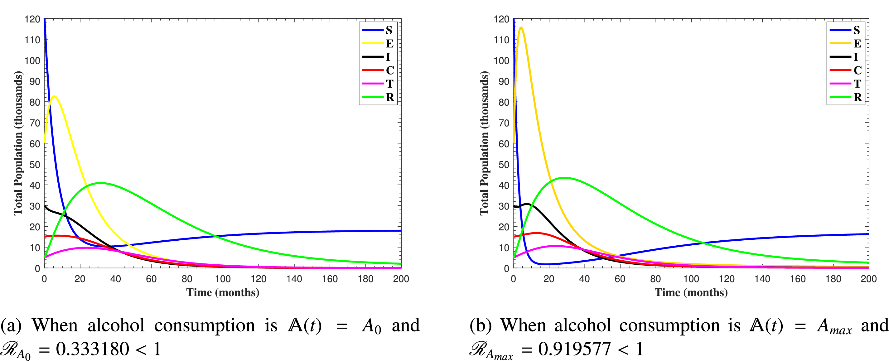
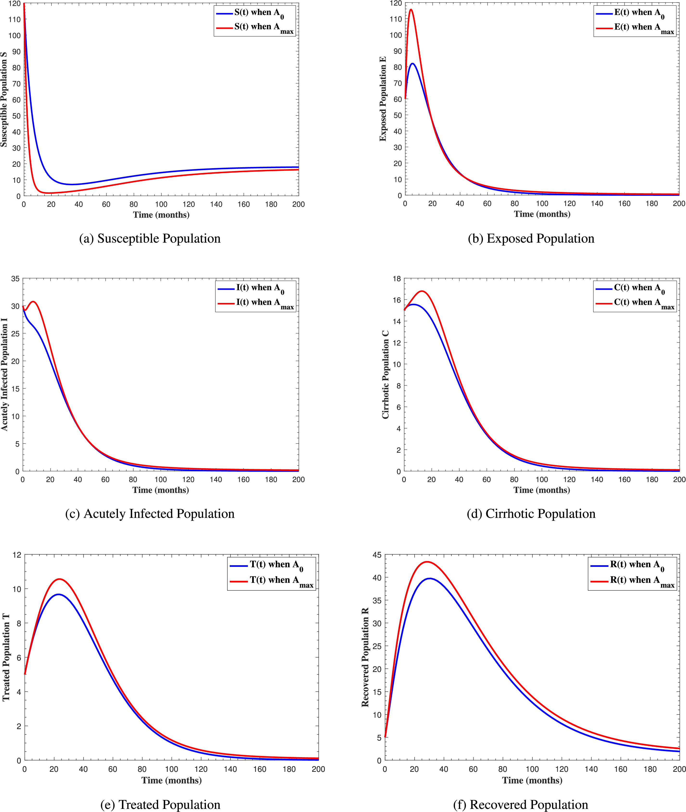
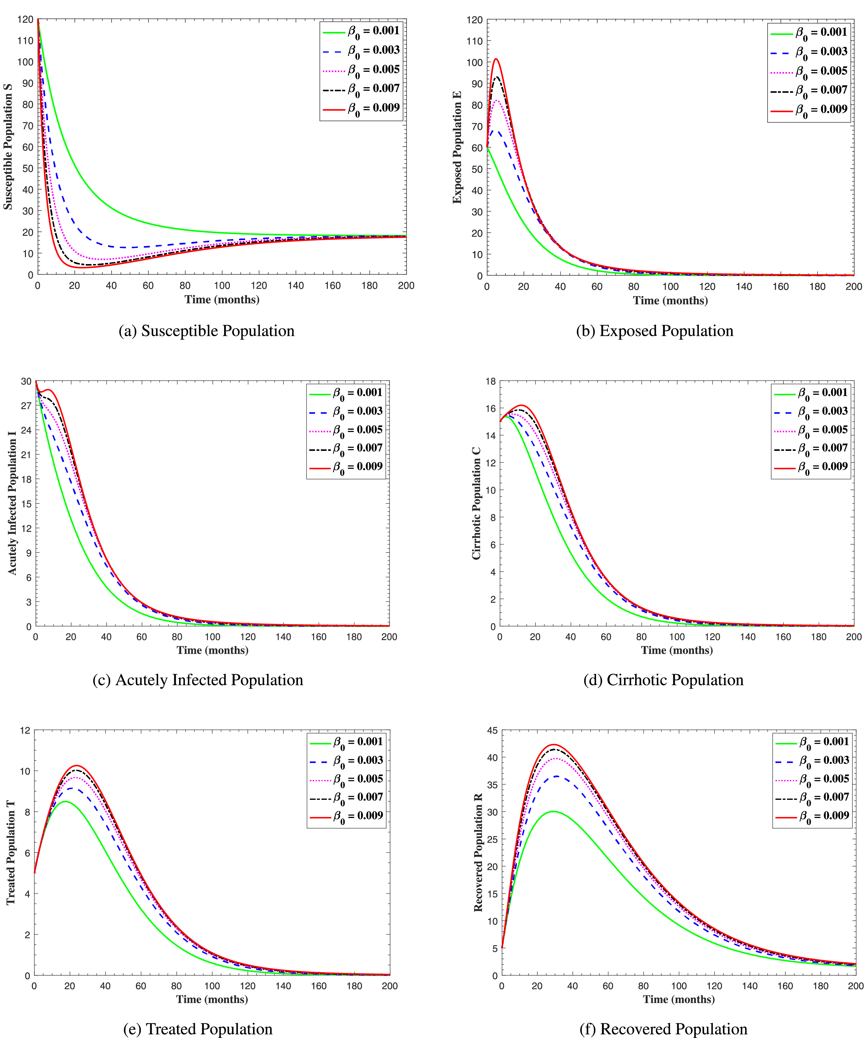
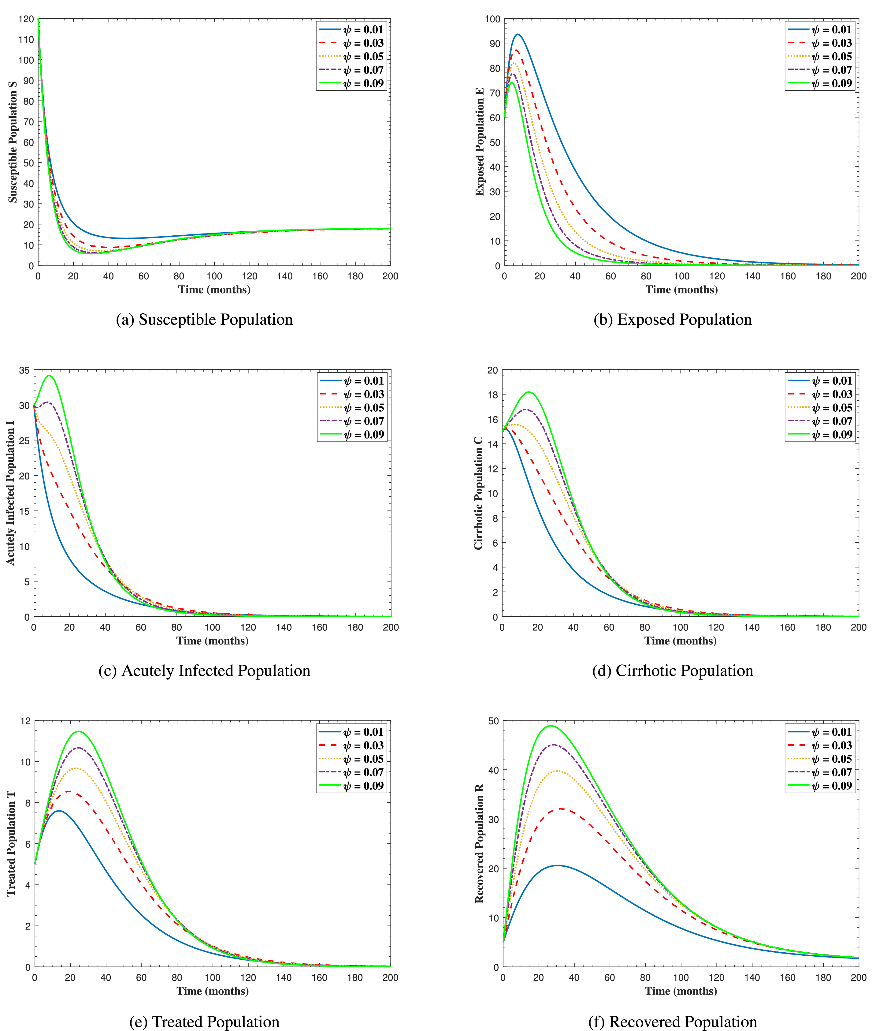
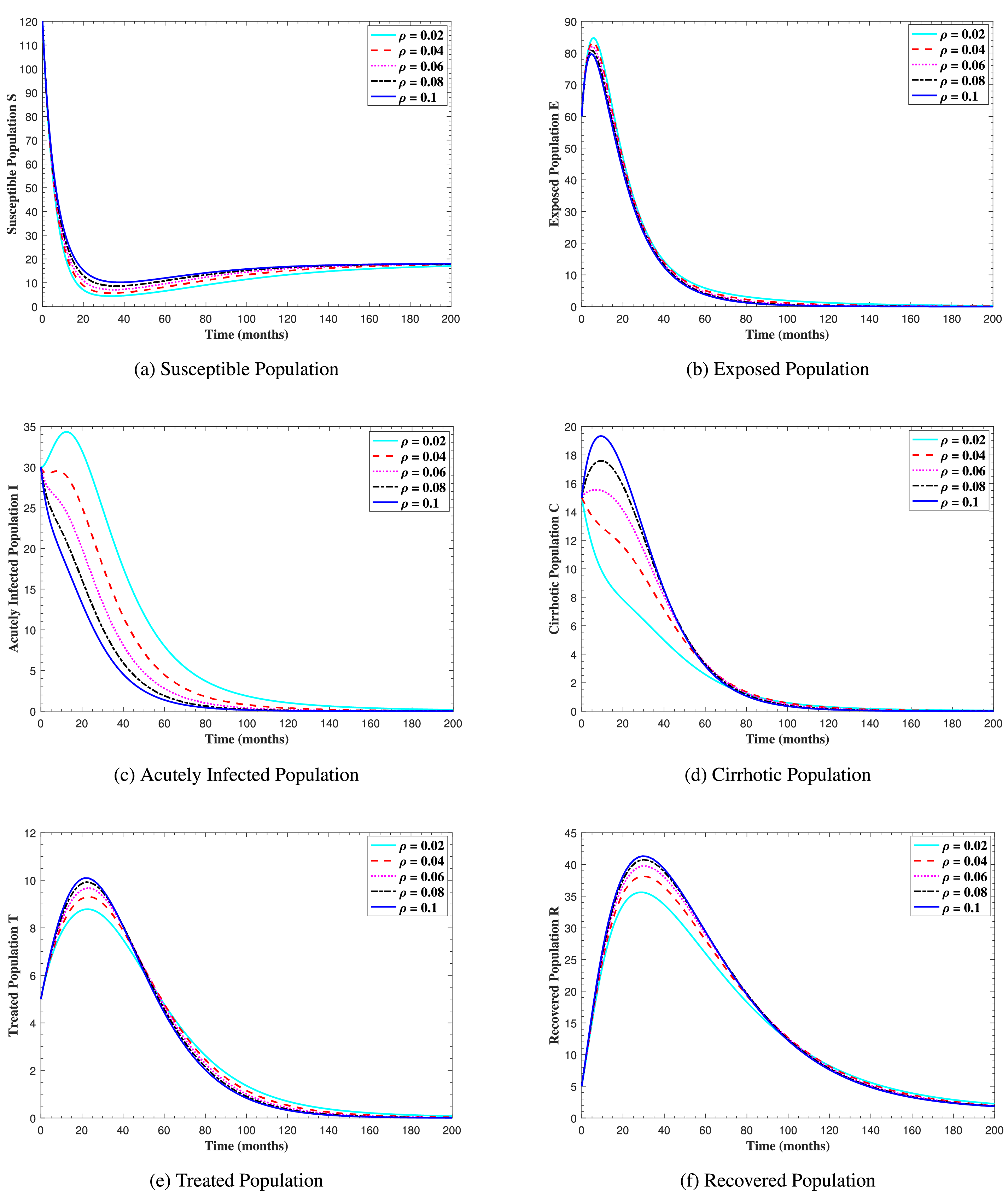
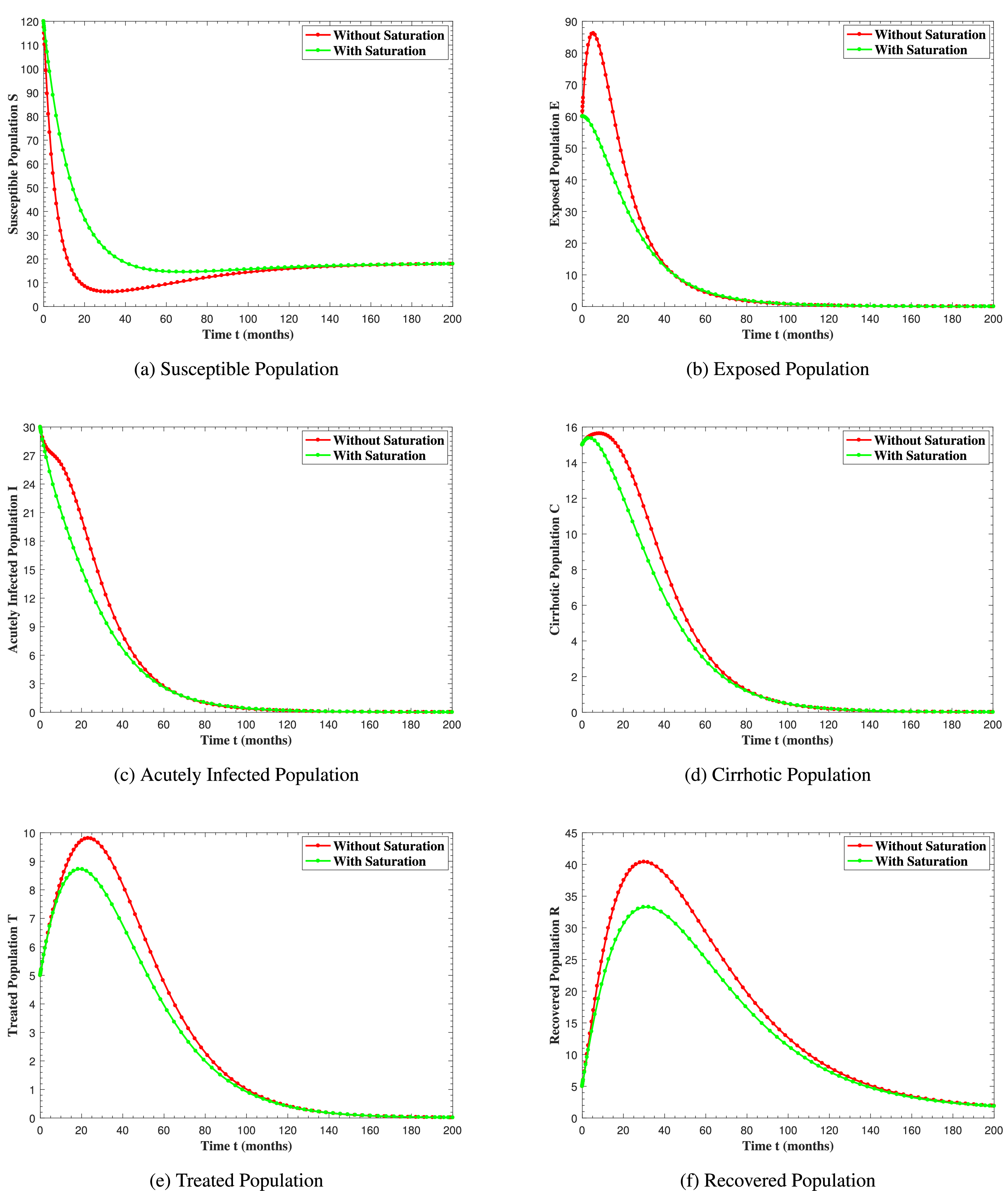
In Fig. 6, the curves represent the dynamic behavior of susceptible, exposed, acutely infected, liver cirrhotic, treated, and recovered individuals. Observing the figure, the susceptible population decreases while the exposed, acutely infected, liver cirrhotic, treated, and recovered populations increase for over 80 months and start falling sharply to zero afterward. In both figures, when low and high amounts of alcohol are consumed, all trajectories are converging to (18.125,0,0,0,0,1.208), verifying the local stability of the disease-free equilibrium of system (1). Fig. 7 shows the impact of alcohol consumption on the progression dynamics of each compartment. As clearly seen from sub-figure (a), as alcohol consumption increases, the number of susceptible individuals decreases, while from sub-figure (b), the exposed individuals increase significantly. From sub-figures (c) and (d), it can be observed that alcohol use by a Hepatitis B-infected individual accelerates the progression of acute infection and liver cirrhosis, respectively. Fig. 8 shows the simulation results for the variation of the baseline transmission rate β0. The Increase in this rate results in an increase in the exposed, acutely infected, and liver cirrhotic population. To minimize the transmission rate, alcohol usage incremental rate should be decreased. Fig. 9 shows the simulation results for the variation of parameter ψ which demonstrates that variations in parameter ψ yields a tremendous change in each compartment. It indicates that if all other model parameters are kept fixed and only varying the parameter ψ, the exposed, acutely infected, and liver cirrhotic individuals increase. Fig. 10 shows the simulation results for the variation of parameter ρ, which yields a dramatic increase in the cirrhotic individuals. Consequently, the acutely infected individuals decrease because they are transferring to the cirrhotic class. It indicates that if only varying the parameter ρ and keeping all other fixed, the liver cirrhotic individuals increases. Fig. 11 shows the simulation results for the saturation parameter α2, which demonstrates that by varying α2, the susceptible individuals increase while exposed, acutely infected, and cirrhotic individuals decrease.
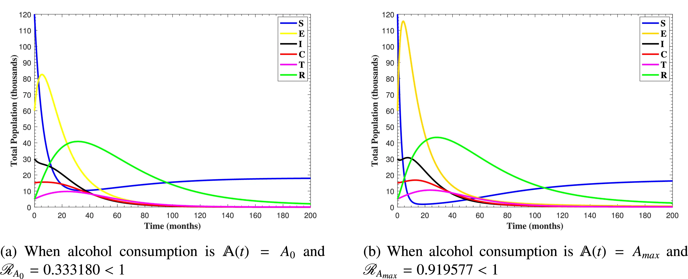
Figure 6: The plots show how all trajectories of the state variables S(t), E(t), I(t), C(t), T(t) and R(t) converge to the disease-free equilibrium
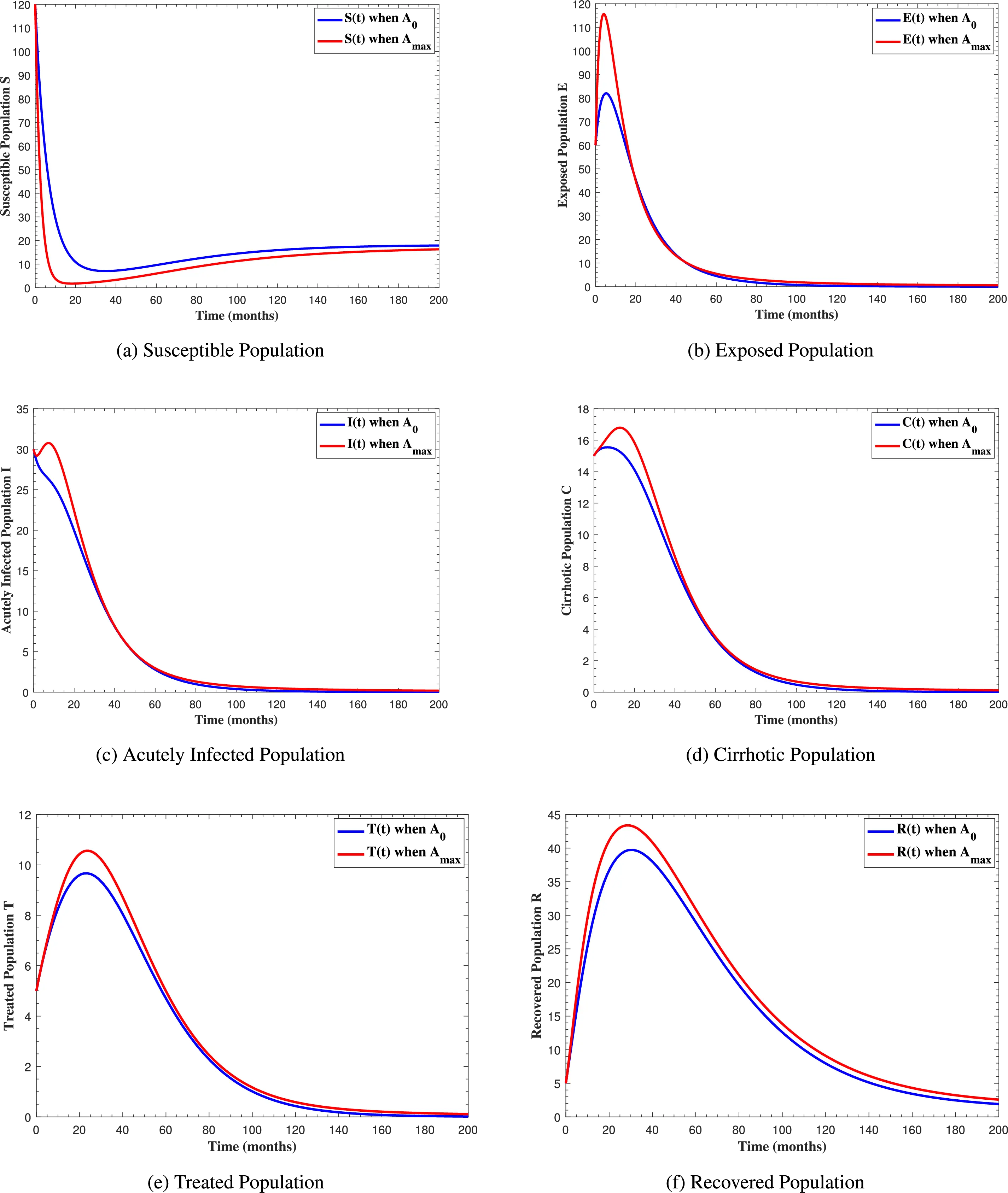
Figure 7: The graphs show the simulation results of S(t), E(t), I(t), C(t), T(t) and R(t)
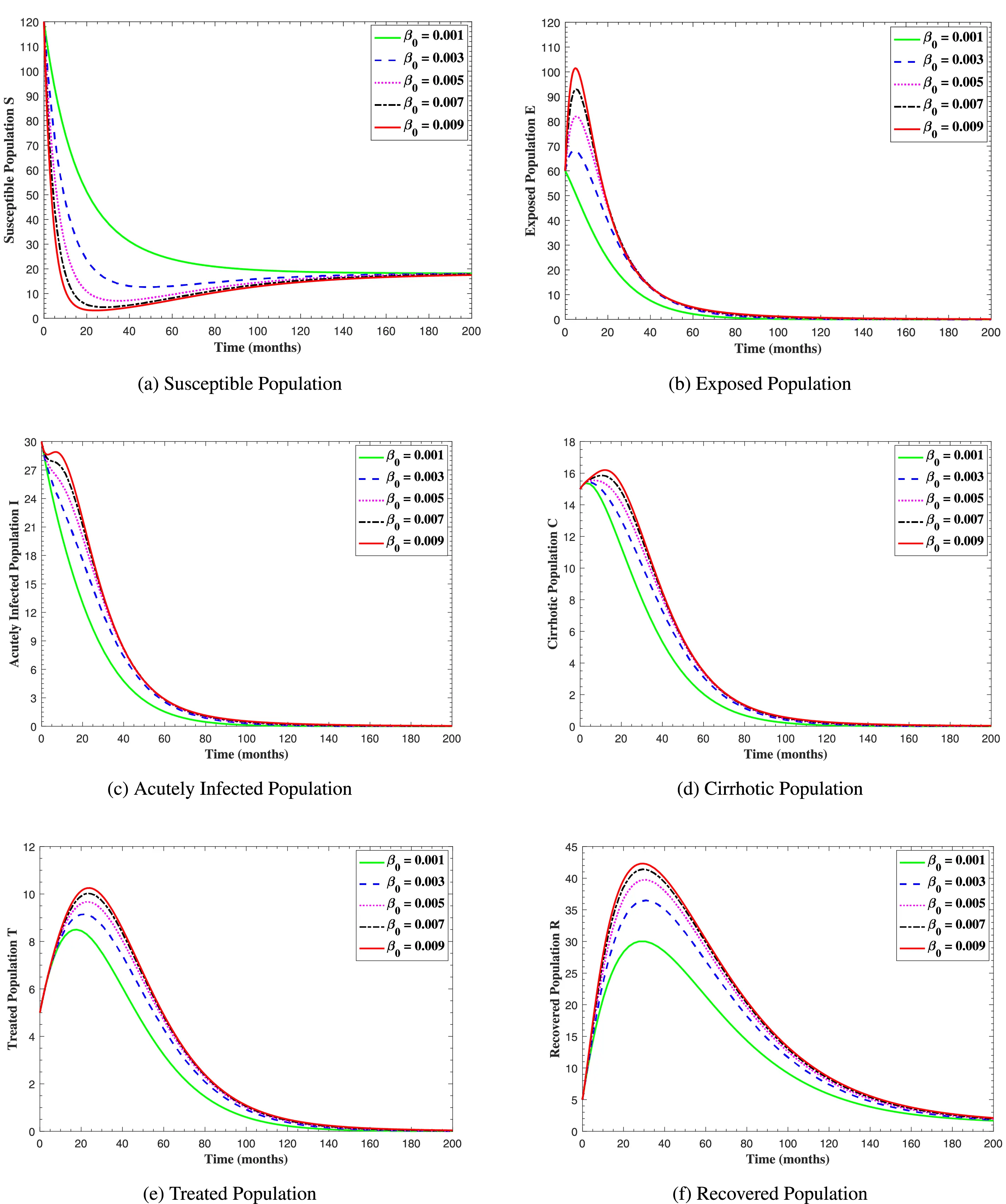
Figure 8: The graphs show the simulation results of S(t), E(t), I(t), C(t), T(t), and R(t) respectively, with respect to various baseline transmission coefficient β0, when all other parameters are kept fixed
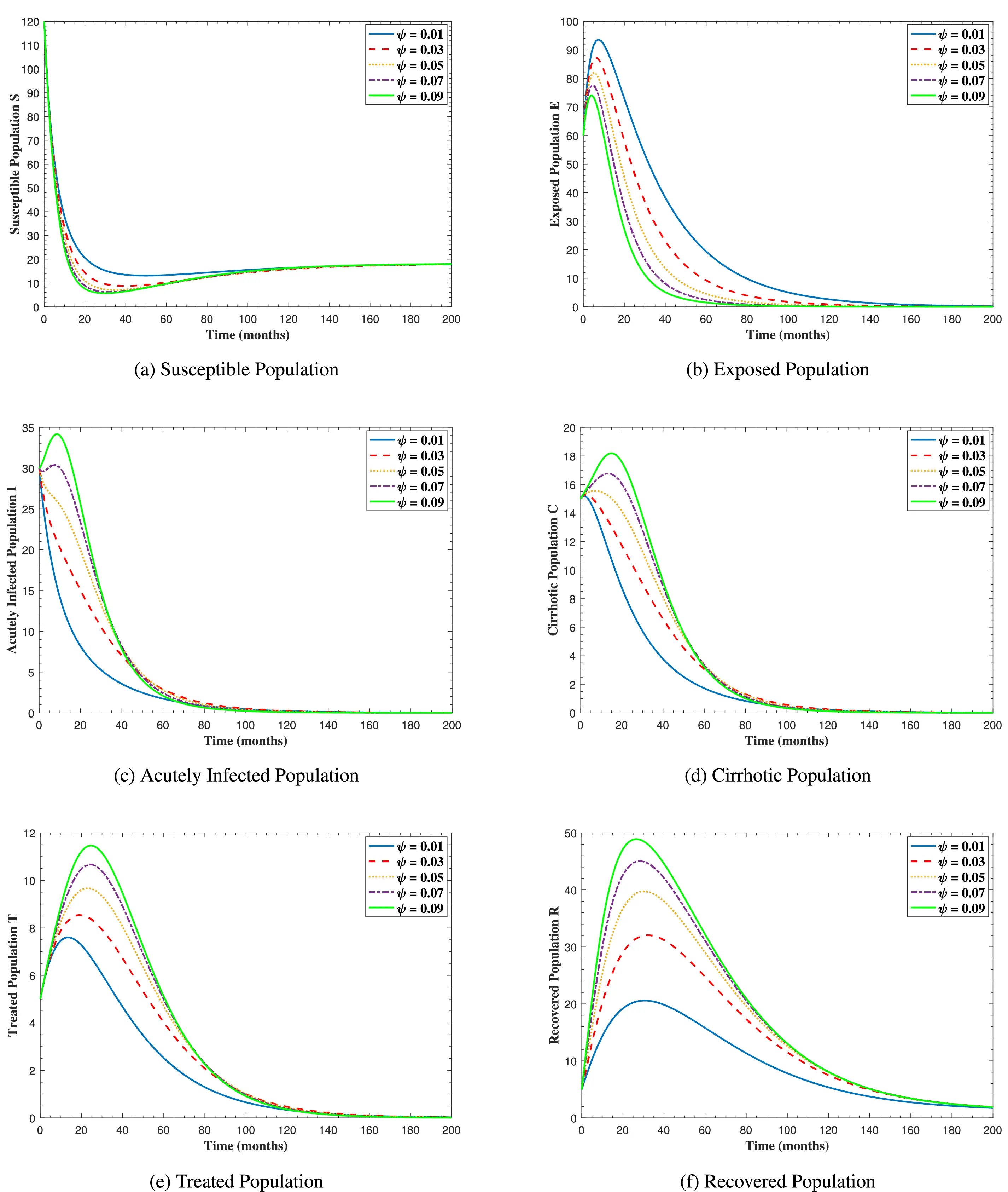
Figure 9: The graphs show the simulation results of S(t), E(t), I(t), C(t), T(t), and R(t) respectively, with respect to various acute infection transmission rate ψ, when all other parameters are kept fixed
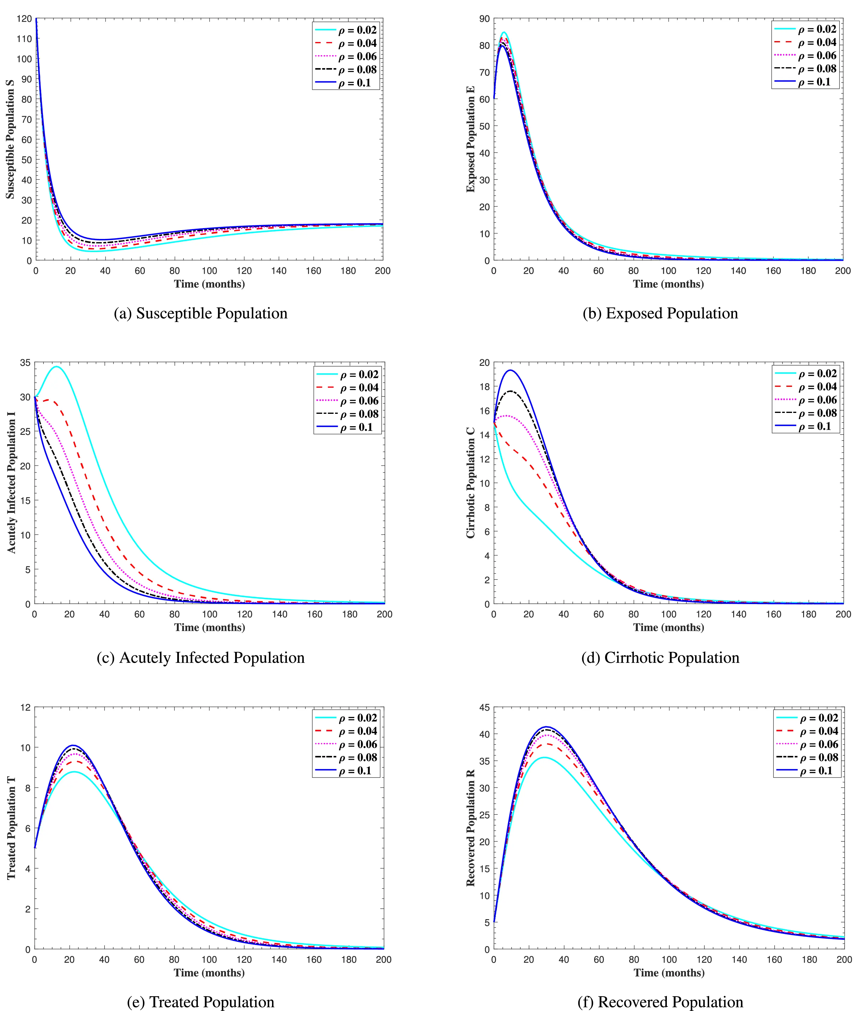
Figure 10: The graphs show the simulation results of S(t), E(t), I(t), C(t), T(t), and R(t) respectively, with respect to various cirrhosis progression rate ρ, when all other parameters are kept fixed
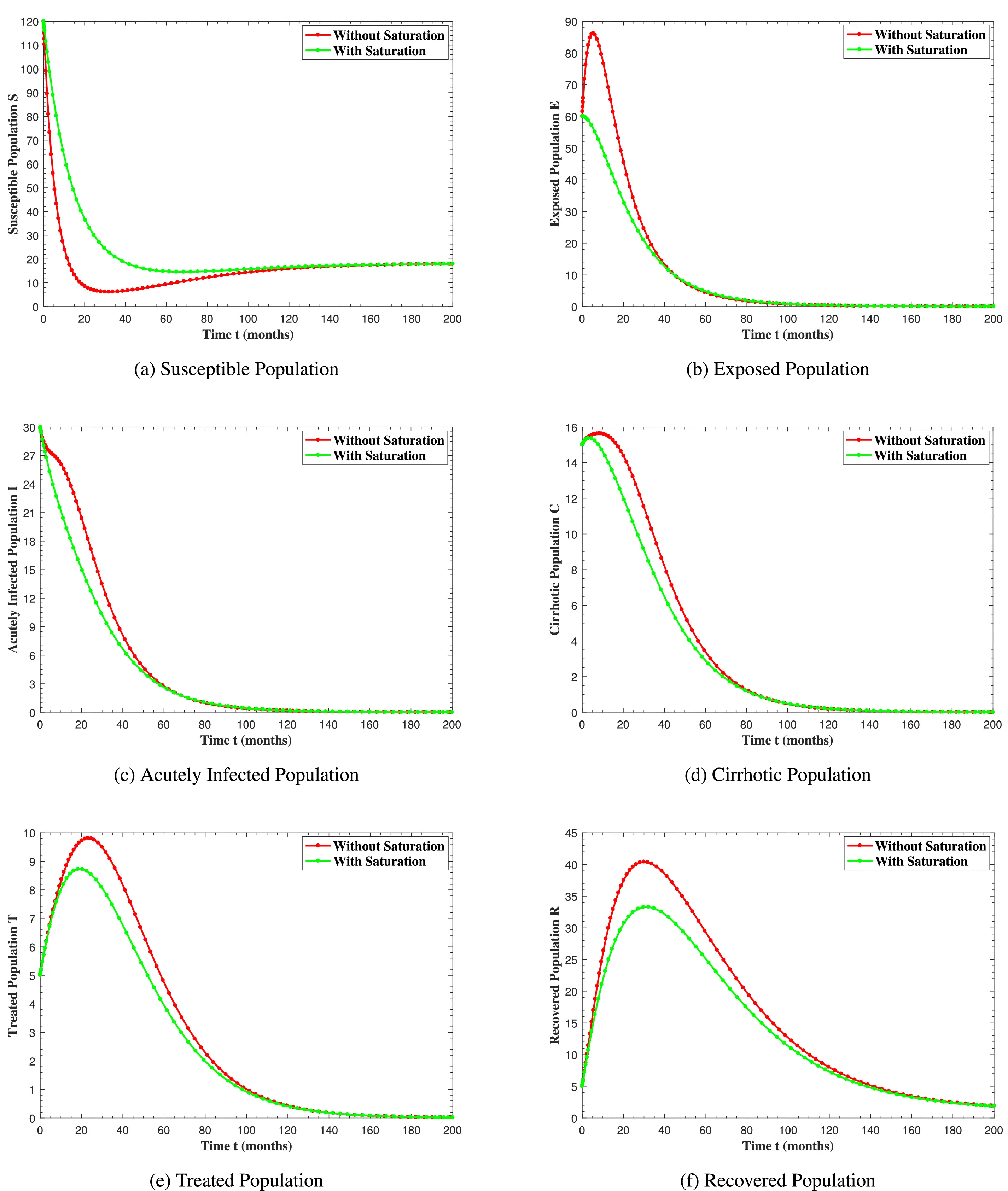
Figure 11: The graphs show the simulation results of S(t), E(t), I(t), C(t), T(t) and R(t) respectively, with saturation and without saturation
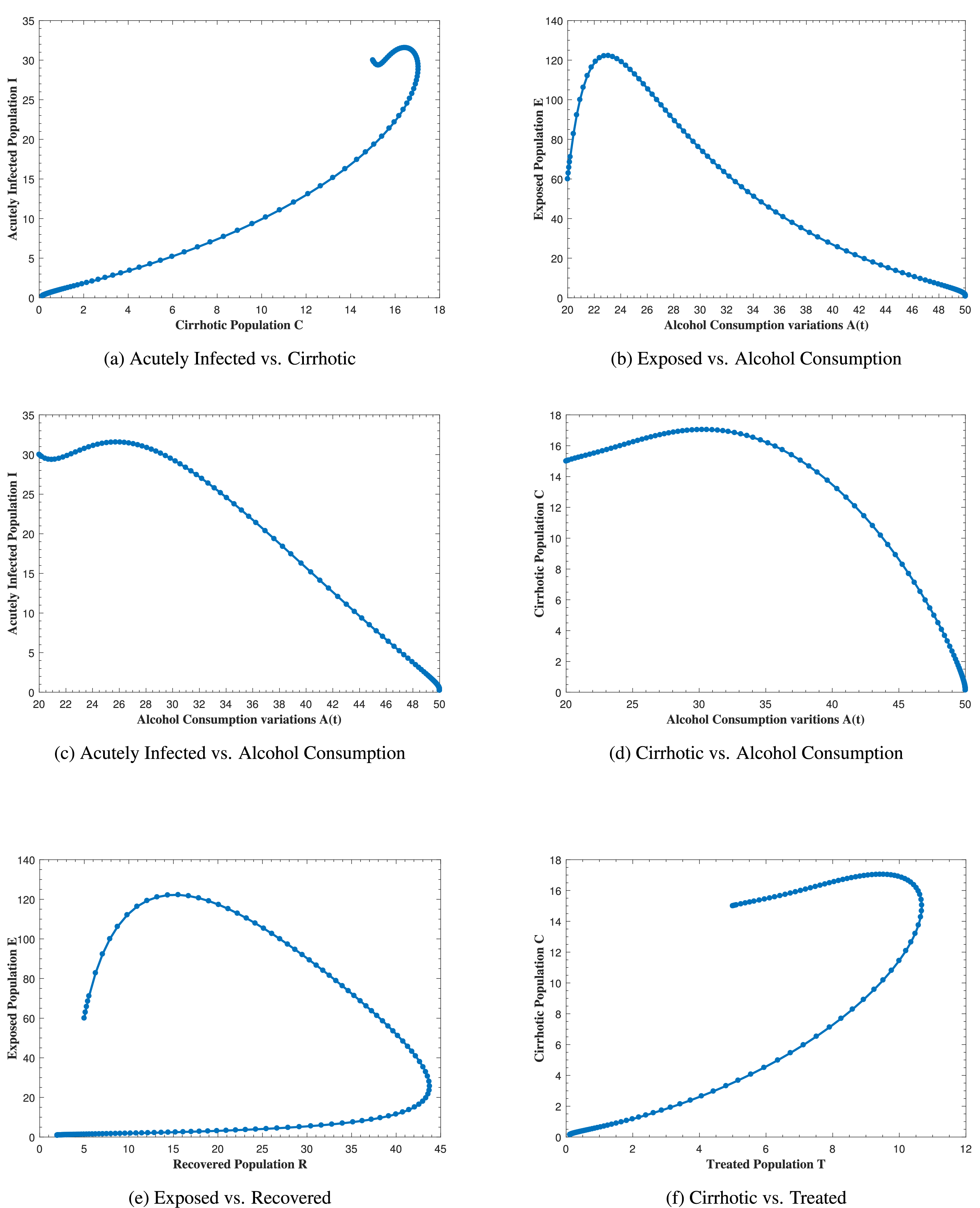
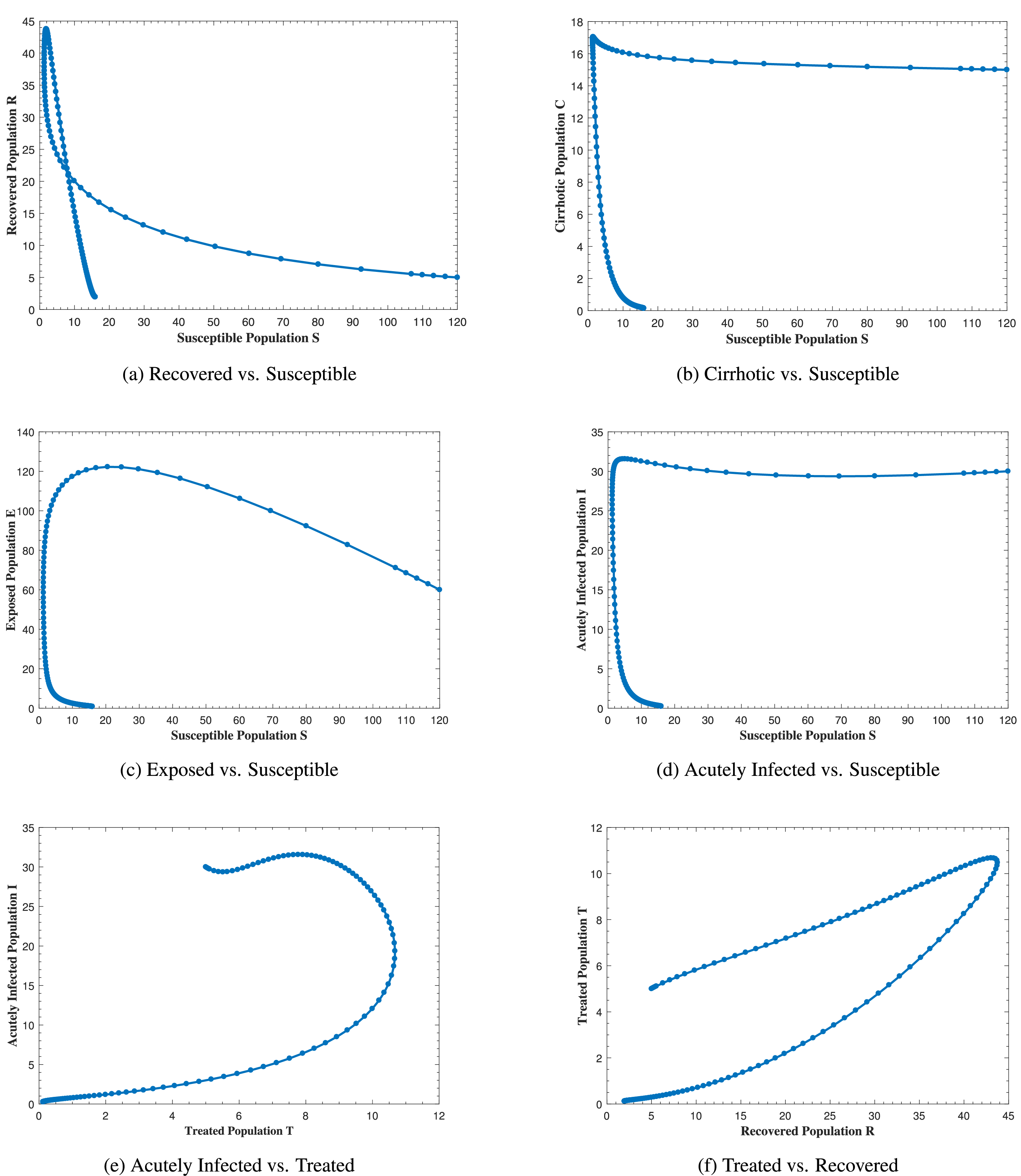
Fig. 12 represents the phase portrait of (a) C(t) vs. I(t), (b) A(t) vs. E(t), (c) A(t) vs. I(t), (d) A(t) vs. C(t), (e) R(t) vs. E(t) and (f) T(t) vs. C(t) with stable disease-free equilibrium and respective values of parameters in Table 1. In Fig. 12a, whenever the number of acutely infected individuals increases, the cirrhotic also increases for the first few months but then sharply converges to zero (the disease-free equilibrium). In Fig. 12b–d, as alcohol consumption increases, the exposed, acutely infected and cirrhotic individuals also increase, respectively for the first few months and start declining afterwards. Fig. 12e demonstrates that, for the first few months, whenever the number of exposed individuals increases, the recovered also increases slightly, but as the exposed individuals start declining, the recovered increases highly and converges to the disease-free equilibrium afterwards. Fig. 12f, shows that whenever the number of cirrhotic people increases, the number of treated people also increases for the first few months, but after some time, both start to decline and converge to the disease-free equilibrium point. Similarly, Fig. 13 shows the phase space diagram of (a) S(t) vs. R(t), (b) S(t) vs. C(t), (c) S(t) vs. E(t), (d) S(t) vs. I(t), (e) T(t) vs. I(t) and (f) R(t) vs. T(t) with stable disease-free equilibrium and respective values of parameters in Table 1.
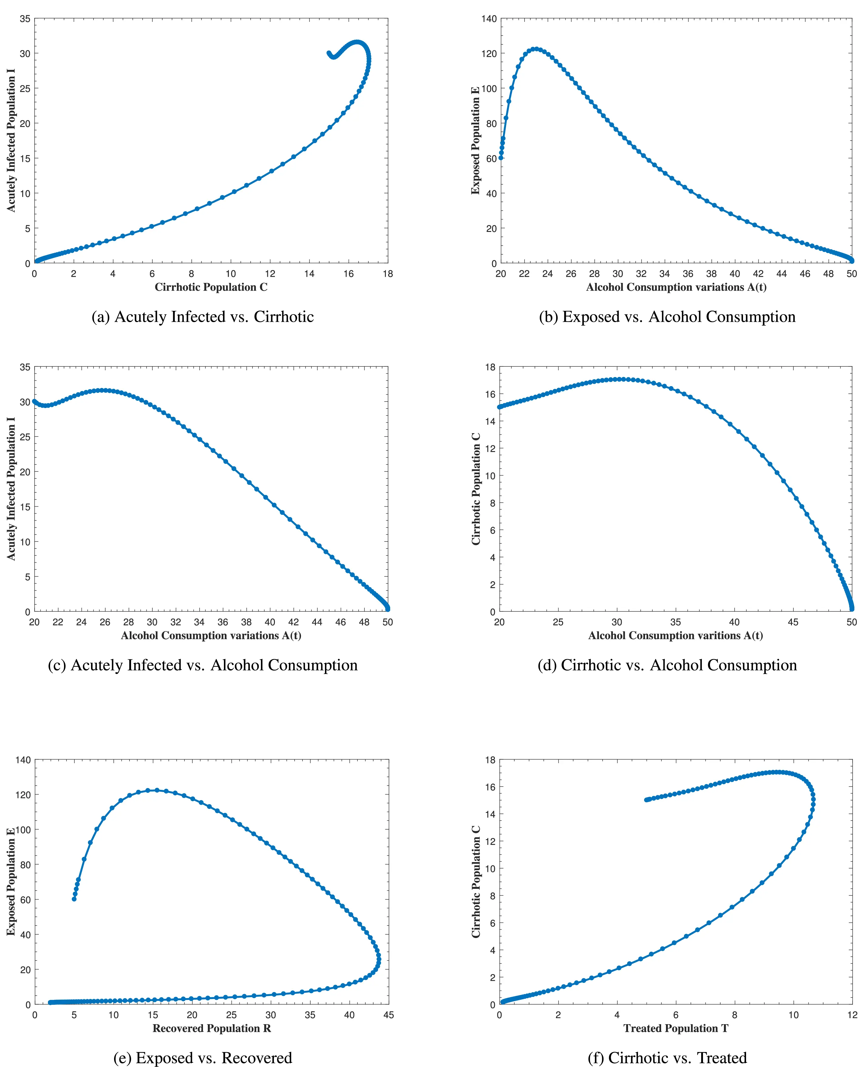
Figure 12: The plot shows the phase space diagram of (a) C(t) vs. I(t), (b) A(t) vs. E(t), (c) A(t) vs. I(t), (d) A(t) vs. C(t), (e) R(t) vs. E(t) and (f) T(t) vs. C(t) with stable disease-free equilibrium
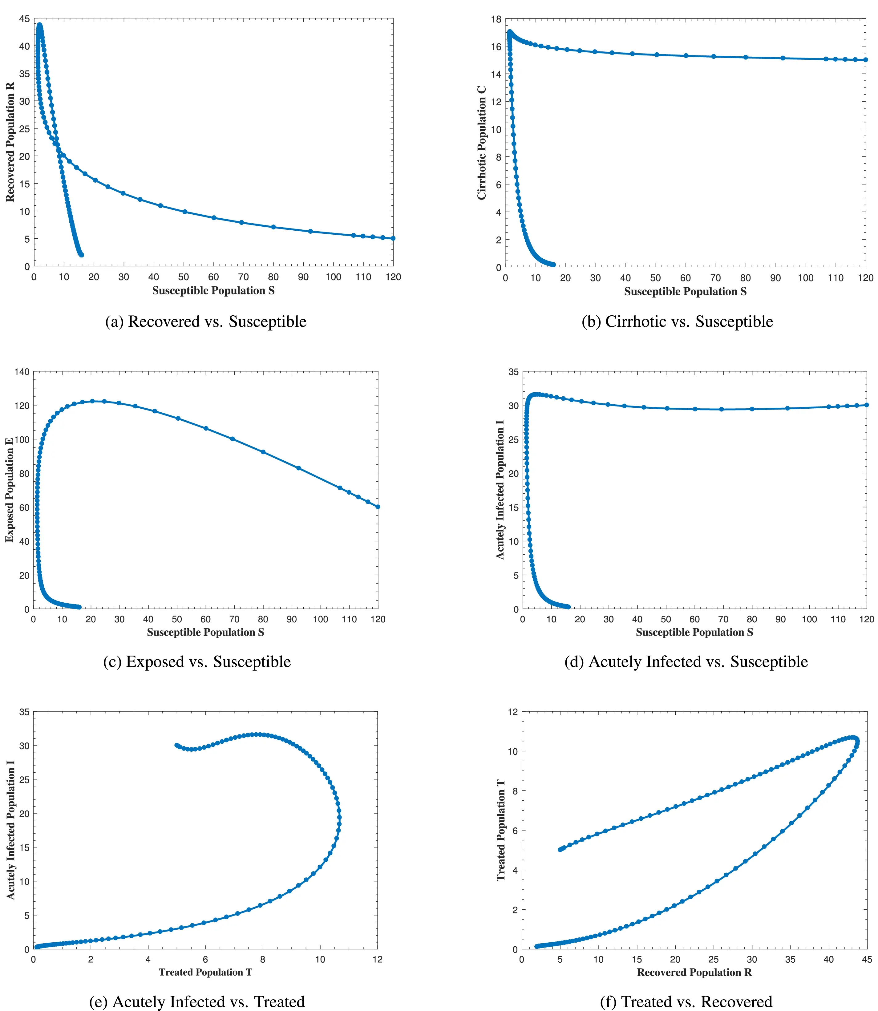
Figure 13: The plot shows the phase space diagram of (a) S(t) vs. R(t), (b) S(t) vs. C(t), (c) S(t) vs. E(t), (d) S(t) vs. I(t), (e) T(t) vs. I(t) and (f) R(t) vs. T(t) with stable disease-free equilibrium
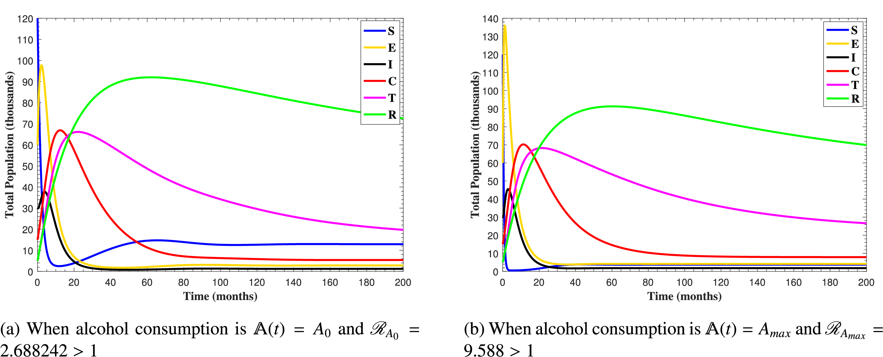
In Fig. 14, the system (1) reaches endemic state by assuming b=0.98, β0=0.04, β1=0.14, μ0=0.01 ν=0.02, ρ=0.25, γ1=0.89, τ1=0.15, and ψ=0.2 with all other parameter values in Table 1, which results ℛ0=[ℛA0,ℛAmax]>1. The susceptible population decreases while all other populations increase, but this pattern persists for a specific duration. After some time, all the trajectories of the system states converge to the endemic equilibrium point. In both figures, all curves remain at these specific values when high or low amount of alcohol is consumed, confirming the stability of the endemic equilibrium point of system (1).
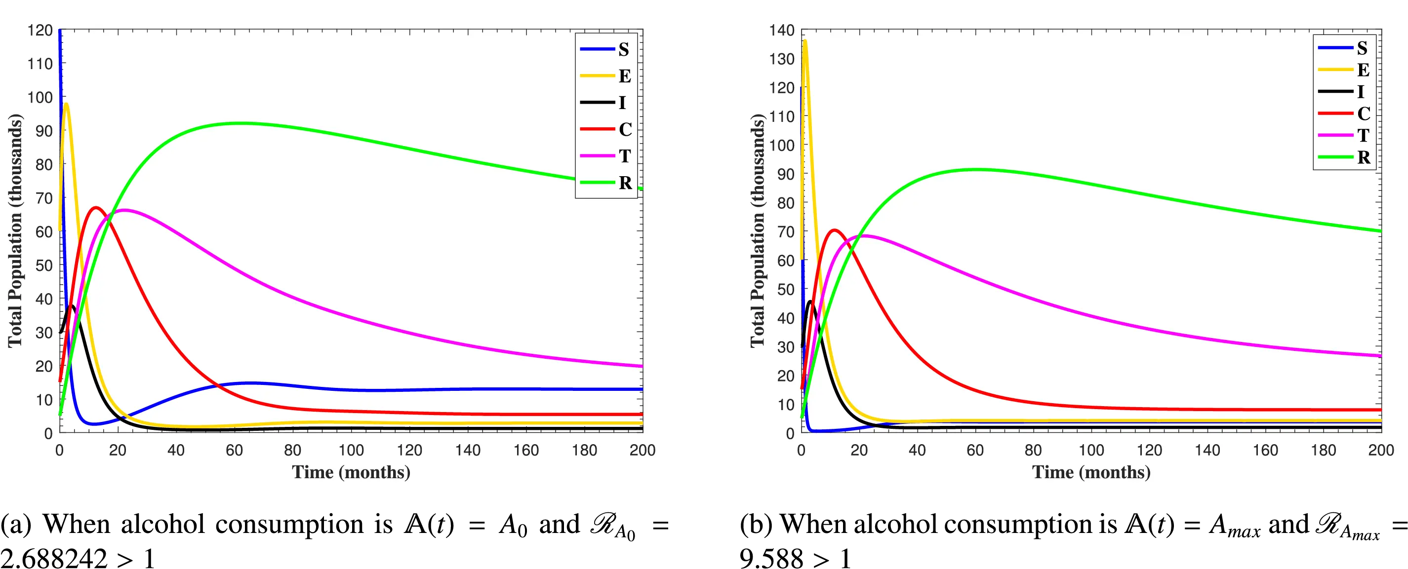
Figure 14: The plots shows how all trajectories of the state variables S(t), E(t), I(t), C(t), T(t) and R(t) converging to endemic equilibrium
8 Conclusion
In this study, the combined effect of heavy alcohol use and Hepatitis B infection on the dynamics of liver cirrhosis development was examined using the idea of a deterministic epidemiological model. A logistic equation was also employed to explain the variability in alcohol intake over time. This model helped in understanding and analyzing various dynamical properties of the combined effect of heavy alcohol use and Hepatitis B infection. In addition, we considered the saturated incidence rate and showed the effect of the saturation parameter on each class. Moreover, a treated compartment was added to see the complex relationships among liver cirrhosis, recovery, and therapy dynamics. The basic characteristics of the proposed model were examined to confirm its viability both mathematically and biologically. The basic reproductive numbers ℛA0 and ℛAmax and the equilibria for both the disease-free and endemic are obtained, as well as the local and global stabilities of the equilibria. The sensitivity analysis was performed and demonstrated the role of every parameter and quantified the most sensitive parameters to the liver cirrhosis transmission. Using central manifold theory and the method of Chavez & Song, we established and proved the existence of forward bifurcation. Ultimately, detailed numerical simulations were conducted for the suggested model, confirming the analytical results. The numerical simulation results reveal that if an alcohol usage reduction program is not implemented, the effects of the combination of heavy alcohol use and Hepatitis B infection will accelerate the progression of liver cirrhosis. However, inhibitory or crowding effects of susceptible and infected individuals, respectively, and treatment of acutely infected individuals may reduce liver cirrhosis progression.
To eradicate liver cirrhosis in the community, any committed researcher is encouraged to apply an optimal control strategy by considering different control variables to reduce the risk of alcohol intake in chronic Hepatitis B carriers. The most significant factor in Hepatitis B transmission is age dependency. Therefore, the same model can be converted into an age-structured model to see the effects of Hepatitis B and liver cirrhosis on different age groups. Furthermore, the same model can be converted to a stochastic model to study random fluctuations and uncertainty in liver cirrhosis progression dynamics.
This study has certain limitations that provide avenues for future research. While the model captures the synergistic dynamics of Hepatitis B and alcohol, it does not incorporate spatial heterogeneity, despite the well-documented geographical variability in Hepatitis B prevalence and alcohol consumption patterns. The current deterministic framework was chosen to establish a foundational, analytically tractable understanding of the core mechanisms. The exclusion of spatial effects allows for a focused analysis on the population-level interactions between disease progression and behavioral factors without the added complexity of regional parameterization and human mobility networks. Future work will aim to extend this model into a spatial or meta-population framework to explore how regional differences in public health policies, vaccination coverage, and cultural norms regarding alcohol use influence the overall burden of liver cirrhosis.
Acknowledgement: Not applicable.
Funding Statement: No funding was received to assist with the preparation of this manuscript.
Author Contributions: Zia Ur Rahman, Formal Analysis; Nigar Ali, Zeeshan Ali, Conceptualization; Dragan Pamucar, Review and Editing; Imtiaz Ahmad, Simulation and Validation; Haci Mehmet Baskonus, Overall Supervision and Review, Naseer Ul Haq, Writing Original Draft; Zeeshan Ali, Methodology, Validation, Resources. All authors reviewed the results and approved the final version of the manuscript.
Availability of Data and Materials: All data that support the findings of this study are included within the article.
Ethics Approval: Not applicable.
Conflicts of Interest: The authors declare no conflicts of interest to report regarding the present study.
References
1. Ginès P, Krag A, Abraldes JG, Solà E, Fabrellas N, Kamath PS. Liver cirrhosis. Lancet. 2021;398(10308):1359–76. [Google Scholar]
2. Khatun MS, Biswas MHA. Optimal control strategies for preventing hepatitis B infection and reducing chronic liver cirrhosis incidence. Infect Dis Model. 2020;5:91–110. doi:10.1016/j.idm.2019.12.006. [Google Scholar] [PubMed] [CrossRef]
3. Canadian Centre for Occupational Health and Safety. Hepatitis B. Hamilton, ON, Canada: Canadian Centre for Occupational Health and Safety; 2024 [cited 2025 May 30]. Available from: www.ccohs.ca/oshanswers/diseases/hepatitisb.html. [Google Scholar]
4. Khan M, Khan T, Ahmad I, Shah Z, Khan A. Modeling of Hepatitis B virus transmission with fractional analysis. Math Probl Eng. 2022;2022(1):6202049. [Google Scholar]
5. World Health Organization. Hepatitis B [Fact sheet]. 2024 [cited 2025 Nov 11]. Available from: http://www.who.int/mediacentre/factsheets/fs204/en/. [Google Scholar]
6. Iida-Ueno A, Enomoto M, Tamori A, Kawada N. Hepatitis B virus infection and alcohol consumption. World J Gastroenterol. 2017;23(15):2651. doi:10.3748/wjg.v23.i15.2651. [Google Scholar] [PubMed] [CrossRef]
7. Ganesan M, Eikenberry A, Poluektova LY, Kharbanda KK, Osna NA. Role of alcohol in pathogenesis of hepatitis B virus infection. World J Gastroenterol. 2020;26(9):883. doi:10.3748/wjg.v26.i9.883. [Google Scholar] [PubMed] [CrossRef]
8. Din A, Li Y, Liu Q. Viral dynamics and control of hepatitis B virus (HBV) using an epidemic model. Alex Eng J. 2020;59(2):667–79. doi:10.1016/j.aej.2020.01.034. [Google Scholar] [CrossRef]
9. Xu HQ, Wang CG, Zhou Q, Gao YH. Effects of alcohol consumption on viral hepatitis B and C. World J Clin Cases. 2021;9(33):10052. doi:10.12998/wjcc.v9.i33.10052. [Google Scholar] [PubMed] [CrossRef]
10. Vonghia L, Leggio L, Ferrulli A, Bertini M, Gasbarrini G, Addolorato, Alcoholism Treatment Study Group. Acute alcohol intoxication. Eur J Internal Med. 2008;19(8):561–7. doi:10.1016/j.ejim.2007.06.033. [Google Scholar] [PubMed] [CrossRef]
11. Khan T, Ullah R, Zaman G, Ahmad I. The analysis of hepatitis B virus (HBV) transmission using an epidemic model. Nat Appl Sci Int J (NASIJ). 2021;2(1):70–9. doi:10.47264/idea.nasij/2.1.6. [Google Scholar] [CrossRef]
12. Lai CL, Yuen MF. The natural history and treatment of chronic hepatitis B: a critical evaluation of standard treatment criteria and end points. Ann Intern Med. 2007;147(1):58–61. doi:10.7326/0003-4819-147-1-200707030-00010. [Google Scholar] [PubMed] [CrossRef]
13. Capasso V, Serio G. A generalization of the Kermack–McKendrick deterministic epidemic model. Math Biosci. 1978;42(1–2):43–61. doi:10.1016/0025-5564(78)90006-8. [Google Scholar] [CrossRef]
14. Azeem M, Jamil MK. On the anticancer drug structures and their locating numbers. Spectrum Oper Res. 2024;1(1):44–63. doi:10.31181/sor1120245. [Google Scholar] [CrossRef]
15. Azeem M, Jamil MK. Constant partition dimension of different anticancer drug structures. Spectrum Decis Making Appl. 2024;1(1):64–83. doi:10.31181/sdmap1120245. [Google Scholar] [CrossRef]
16. Zhou L, Fan M. Dynamics of an SIR epidemic model with limited medical resources revisited. Nonlinear Anal: Real World Appl. 2012;13(1):312–24. doi:10.1016/j.nonrwa.2011.07.036. [Google Scholar] [CrossRef]
17. Ilhan Ö, Şahin G. A numerical approach for an epidemic SIR model via Morgan-Voyce series. Int J Math Comput Eng. 2024;2(1):125–40. doi:10.2478/ijmce-2024-0010. [Google Scholar] [CrossRef]
18. Park B, Jung KW, Oh CM, Choi KS, Suh M, Jun JK. Factors associated with alcohol consumption in hepatitis B carriers: a nationwide study in the Republic of Korea. PLoS One. 2014;9(11):e110144. doi:10.1371/journal.pone.0110144. [Google Scholar] [PubMed] [CrossRef]
19. Khajji B, Labzai A, Balatif O, Rachik M. Mathematical modeling and analysis of an alcohol drinking model with the influence of alcohol treatment centers. Int J Math Math Sci. 2020;2020(1):4903168. doi:10.1155/2020/4903168. [Google Scholar] [CrossRef]
20. Shah I, Ali I, Ali A, Ahmad I, Islam S, Rasool G, et al. Optimal control and sensitivity analysis of a mathematical model for MDR-TB transmission with advanced treatment strategies. Eur Phys J Plus. 2025;140(6):1–15. doi:10.1140/epjp/s13360-025-06486-8. [Google Scholar] [CrossRef]
21. Chawla SR, Ahmad S, Albalawi W, Khan A, Shah I, Eid MR. Stability analysis of a modified general SEIR model with harmonic mean type of incidence rate. Alexandria Eng J. 2025;127:1183–92. doi:10.1016/j.aej.2025.07.006. [Google Scholar] [CrossRef]
22. Zhou E, Yang C, Gao Y. Effect of alcohol on the progress of hepatitis B cirrhosis. Ann Palliat Med. 2021;10(1):415–24. doi:10.21037/apm-20-2353. [Google Scholar] [PubMed] [CrossRef]
23. Dano LB, Rao KP, Keno TD. Modeling the combined effect of hepatitis B infection and heavy alcohol consumption on the progression dynamics of liver cirrhosis. J Math. 2022;2022(1):6936396. doi:10.1155/2022/6936396. [Google Scholar] [CrossRef]
24. Izgi ZP. Simulation studies on the hemodynamic model for blood flow. Int J Math Comput Eng. 2024;3(1):75–82. doi:10.2478/ijmce-2025-0007. [Google Scholar] [CrossRef]
25. Farhan M, Shah Z, Ling Z, Shah K, Abdeljawad T, Islam S, et al. Global dynamics and computational modeling for analyzing and controlling hepatitis B: a novel epidemic approach. PLoS One. 2024;19(6):e0304375. doi:10.1371/journal.pone.0304375. [Google Scholar] [PubMed] [CrossRef]
26. Bruha R, Dvorak K, Petrtyl J. Alcoholic liver disease. World J Hepatol. 2012;4(3):81. [Google Scholar] [PubMed]
27. Ullah I, Ahmad I, Ali N, Ahmad H, Haq IU. Mathematical modeling and analysis of dynamics of neisseria gonorrhea disease with self-protection, treatment and natural immunity. Glob J Sci. 2024;1(1):40–55. doi:10.48165/gjs.2024.1105. [Google Scholar] [CrossRef]
28. Van den Driessche P, Watmough J. Reproduction numbers and sub-threshold endemic equilibria for compartmental models of disease transmission. Math Biosci. 2002;180(1–2):29–48. doi:10.1016/s0025-5564(02)00108-6. [Google Scholar] [PubMed] [CrossRef]
29. Khan MA, DarAssi MH, Ahmad I, Seyam NM, Alzahrani E. Modeling the dynamics of tuberculosis with vaccination, treatment, and environmental impact: fractional order modeling. Comput Model Eng Sci. 2024;141(2):1365–94. doi:10.32604/cmes.2024.053681. [Google Scholar] [CrossRef]
30. Ndendya JZ, Leandry L, Kipingu AM. A next-generation matrix approach using Routh-Hurwitz criterion and quadratic Lyapunov function for modeling animal rabies with infective immigrants. Healthcare Anal. 2023;4:100260. doi:10.1016/j.health.2023.100260. [Google Scholar] [CrossRef]
31. Mahardika R, Widowati, Sumanto YD. Routh-hurwitz criterion and bifurcation method for stability analysis of tuberculosis transmission model. J Phys Conf Series. 2019;1217(1):012056. doi:10.1088/1742-6596/1217/1/012056. [Google Scholar] [CrossRef]
32. Jehangir H, Ali N, Ahmad I, Younas H, Ahmad Z, El-Agamy RF. Global dynamics and numerical simulation of a vaccinated mathematical model for rabies disease. Glob J Sci. 2024;1(1):14–27. [Google Scholar]
33. LaSalle JP. Stability theory and invariance principles. In: Dynamical systems. New York, NY, USA: Academic Press; 1976. p. 211–22. [Google Scholar]
34. Vanderbauwhede A, Iooss G. Center manifold theory in infinite dimensions. In: Dynamics reported: expositions in dynamical systems. Berlin/Heidelberg, Germany: Springer; 1992. p. 125–63. [Google Scholar]
35. Castillo-Chavez C, Song B. Dynamical models of tuberculosis and their applications. Math Biosci Eng. 2004;1(2):361–404. doi:10.3934/mbe.2004.1.361. [Google Scholar] [PubMed] [CrossRef]
36. Buonomo B, Lacitignola D. On the backward bifurcation of a vaccination model with nonlinear incidence. Nonlinear Anal Model Control. 2011;16(1):30–46. doi:10.15388/NA.16.1.14113. [Google Scholar] [CrossRef]
37. Chitnis N, Hyman JM, Cushing JM. Determining important parameters in the spread of malaria through the sensitivity analysis of a mathematical model. Bull Math Biol. 2008;70:1272–96. doi:10.1007/s11538-008-9299-0. [Google Scholar] [PubMed] [CrossRef]

 Submit a Paper
 Propose a Special lssue
 Open Access
 View Full Text
 Download PDF
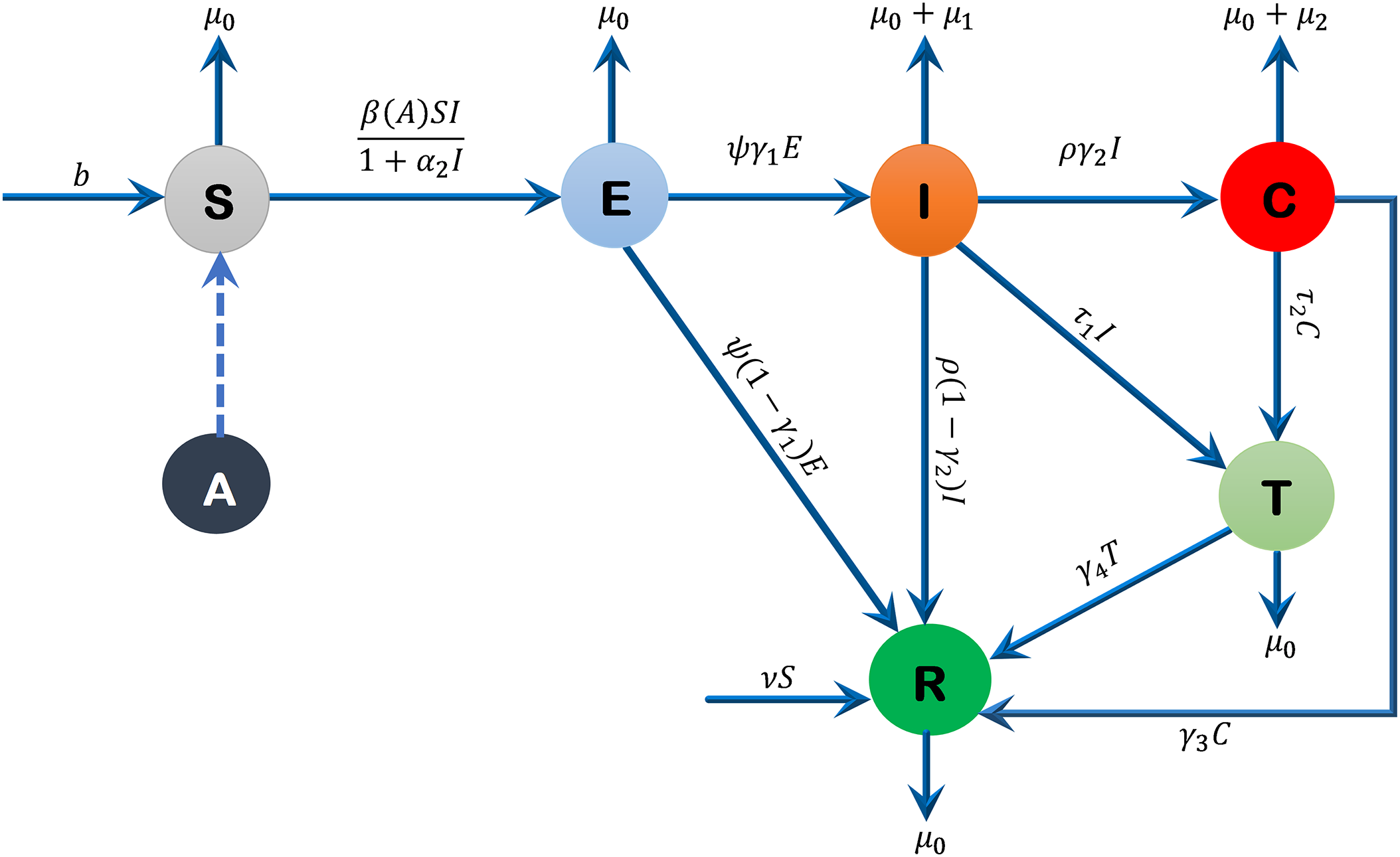


 Copyright © 2026 The Author(s). Published by Tech Science Press.
 Downloads
 Citation Tools