Geometrically Nonlinear Analyses of Isotropic and Laminated Shells by a Hierarchical Quadrature Element Method

1  Introduction

Nonlinear shell analysis has long been a subject of extensive research [1], owing to its critical role in a wide range of engineering fields such as aerospace, civil architecture, and automotive design. Although the mathematical foundations of shell theory were laid well before the advent of modern computational mechanics, its notoriously intricate formulations have historically posed considerable challenges for numerical implementation [2]. A major breakthrough came in 1989 when Simo and Fox [3] developed the geometrically exact shell theory based on Cosserat’s hypothesis [4] and Mindlin-Reissner theory [5]. This shell model only requires a mid-surface’s position vector and an inextensible director to describe the configuration, with the exclusion of drilling rotations. Since the introduction of the geometrically exact shell model, considerable efforts have been devoted to advancing its theoretical framework. Ibrahimbegović established a finite rotation-based stress resultant framework and addressed singularity issues through vector-like parameterizations [6]. Zhang et al. [7] developed a nonlocal geometrically exact shell theory for fracture modeling under finite deformations. Ma et al. [8] introduced a phase-field fracture model for stress-resultant geometrically exact shells within the finite deformation regime. Parallel to these, the development of the finite element method has been a central theme for improving numerical accuracy and mitigating locking effects. In this context, Zhang et al. [9] introduced a weak-form quadrature element method (QEM), which improves computational efficiency through direct numerical integration at collocation points. Lavrenčič et al. [10] systematically compared mixed and hybrid finite element formulations based on variational principles such as Assumed Natural Strain and Hu–Washizu functionals, aiming to identify optimal approaches for approximating shell behavior. More recently, Kim et al. [11] applied isogeometric analysis with Bézier extraction and assumed natural strain methods, further bridging geometric modeling and high-order finite element analysis.

In practical engineering, the finite element method (FEM) based on geometrically exact formulations has been extensively applied to model the nonlinear response of shells under large deformations [12]. Representative applications include structural stability in advanced materials and structures [13], the nonlinear dynamic analysis of fiber-reinforced composite shell [14], the modeling of curved thin-walled structures with deformable cross-sections [15,16], the simulation of the contact of composite laminates [17], as well as complex failure phenomena in large deformation [18]. Moreover, contemporary shell modeling is being reshaped by broader computational mechanics trends. One major trend is the incorporation of machine learning into the finite element analysis workflow, for purposes ranging from integrating nonlinear shell analysis into design frameworks [19] to merge pattern recognition with a finite element model [20]. Simultaneously, the push for higher computational efficiency has established GPU-accelerated solvers as a critical performance enabler, with demonstrated successes in stamping simulation using shell elements [21] and in explicit dynamics for thin shells [22].

Despite these advancements, practical engineering applications face notable challenges. Low-order elements are widely used but hindered by high computational costs and locking effects. To address these limitations, high-order methods have emerged. In the past decades, the hierarchical finite element method [23], meshfree method [24,25], weak form quadrature element method [26,27], iso-geometric analysis (IGA) [28,29], spectral elements [30,31] and other high-order schemes have begun to emerge for large-scale engineering analyses with high accuracy. However, high-order methods often introduce a new set of challenges, such as meshing difficulties for complex geometries and cumbersome stiffness formulations, presenting a hurdle for practical application. In this context, the Hierarchical Quadrature Element Method (HQEM) was developed to address the implementation difficulties of the hierarchical finite element method, particularly in imposing boundary conditions and assembling elements, by introducing interpolative bases based on differential quadrature nodes along element boundaries [32]. Consequently, the HQEM offers a great balance between computational efficiency and implementation practicality. Further compounding these numerical challenges is the growing need for formulations capable of handling laminated composites, which are increasingly used in lightweight and high-performance structures [33,34]. Extending existing models to laminate materials, however, introduces further complexities in constitutive integration and stress resultant computations, necessitating a mathematically concise and computationally efficient formulation for the nonlinear analysis of complex shell structures undergoing large deformations.

To meet this need, this work presents an extension of the Hierarchical Quadrature Element Method (HQEM) [32] to the nonlinear analysis of both isotropic and laminated shells. By leveraging high-order approximation [35] and hierarchical structure [32], HQEM inherently mitigates shear and membrane locking and readily enables local p-refinement. Notably, the HQEM has demonstrated versatility across various engineering applications. Its applications range from the dynamic analysis of rotor systems [36] and the multi-physics reliability assessment of conical shells [37], to thermo-mechanical fracture simulation with efficient remeshing [38,39]. The key contributions of this work are summarized as follows: (1) a unified HQEM formulation for geometrically exact isotropic and laminated shells; (2) significant simplification of residual force and stiffness matrix computations; (3) inherent mitigation of shear and membrane locking; (4) convenient support for local p-refinement; (5) compared with the weak-form quadrilateral element (QEM) approach [9], accurate capture of nonlinear behavior under high loads; and (6) flexible mesh generation through the combination of quadrilateral and triangular elements. While the current formulations are applied to linear elastic laminates, the HQEM framework can be extended to accommodate more complex scenarios, such as those involving plasticity and functionally graded materials, by introducing appropriate inelastic material models. These extensions will be explored in future work.

The organization of this paper is as follows: Section 2 introduces a brief review of geometrically exact shell theory and constitutive relations of laminated shells. Section 3 introduces the rotation description, updating of the current director with quaternions. Section 4 introduces the shape function of quadrilateral/trilateral HQEM and develops the stress resultant formulation within the HQEM framework, subsequently deriving the corresponding residual force vectors and tangent stiffness matrices. In Section 5, seven benchmark problems are analyzed to confirm the accuracy and convergence of the HQEM. Finally, Section 6 presents the conclusions of the study.

2  Geometrically Exact Shells Model

In the geometrically exact shell model, the shell’s configuration is defined by its mid-surface position and an associated unit director field. As illustrated in Fig. 1, a Cartesian reference frame {ei}(i=1,2,3) is introduced, where r denotes the mid-surface position vector, and t represents the unit director. The current and initial configurations are labeled as Ω and Ω0, respectively. The current configuration of a quadrilateral shell patch is then fully described by

Ω={ϕ⊂R3|ϕ=r(xα)+x3t(xα),α=1,2 and x3∈[h−,h+]}(1)

where x𝛼 (𝛼 = 1, 2) are convected coordinates describing the midsurface of the shell, and the x3 is the thickness coordinate. The thickness of the shell is defined by h=h+−h−. For the ease of representing the deformation gradient of the shell, the current covariant frames Gi (i = 1, 2, 3) and initial covariant frames gi (i = 1, 2, 3) are defined as

{G1G2G3}={r,1+x3t,1r,2+x3t,2t}(2)

and

{g1g2g3}={r0,1+x3t0,1r0,2+x3t0,2t0}(3)

where r0 and r denote the mid-surface position vectors in the initial and current configurations, respectively; t0 and t are the corresponding unit directors. Subscript, (α) indicates partial derivatives with respect to the coordinates xα (α = 1, 2). The differentiation of the mid-surface in the initial configuration is defined as

dΩ0=j0dx1dx2(4)

in which j0=‖r01×r02‖ is the projection parameter in the initial configuration. With the definition of deformation gradient F

F=∇ϕ(∇ϕ)−1=Gi⊗gi(5)

where gi is the contravariant basis vector of gi, satisfying gi·gj = δij, with δij being the Kronecker delta. The Green–Lagrange strain tensor ε can be obtained as

ε=12(FTF−I)=12(Gi⋅Gj−gi⋅gj)gi⊗gj=εijgi⊗gj(6)

and the strain component εij can also be written as

εij=εij(0)+x3εij(1)+(x3)2εij(2)(7)

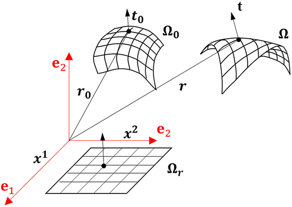
Figure 1: Initial and current configurations of shell

Given the negligible effect of transverse shear gradients in this context [40], the quadratic terms in x3 can be omitted from Eq. (7). Meanwhile, the retained strain components align with those established by Simo et al. [41]. The explicit expressions of the strain component are

εαβ(0)=12(r,α⋅r,β−r,α0⋅r,β0)εα3(0)=ε3α(0)=12r,α⋅tεαβ(1)=12(r,α⋅t,β+r,β⋅t,α−r,α0⋅t,β0−r,β0⋅t,α0)(8)

The relationship between strain ε and stress s can be expressed as:

s(α)=Dε(α),α=0,1(9)

in which the vector forms of strain ε measures and stress s resultants are given as

s=[s11s22s12s13s23]Tε=[ε11ε222ε122ε132ε23]T(10)

A laminated composite shell is composed of a finite number of stacked thin layers with individual material properties along its thickness direction. As shown in Fig. 2, a local Cartesian material frame {eα} (α=1,2,3) is defined on the layer’s initial configuration, with its base vectors e1 and e2 aligned with the fiber’s longitudinal and transverse directions, respectively. For a certain single layer, the homogeneous orthotropic linear elastic constitutive relationship is assumed for material modeling. The constitutive matrix D of pth layer is thus obtained as

D(p)=LD¯LT(11)

where

D¯=[1/E1−υ12/E1000−υ12/E11/E2000001/G12000001/G13000001/G23]−1(12)

L=[(g11)2(g21)22g11g2100(g12)2(g22)22g12g2200g11g12g21g22g12g21+g22g1100000g11g21000g12g22](13)

in which gαβ = eα·gβ. E, υ and G denote the Young’s modulus, Poisson’s ratio, and shear modulus of the material. As depicted in Fig. 2, the vectors eα and the base vectors gα, gα all lie in the plane normal to t0.

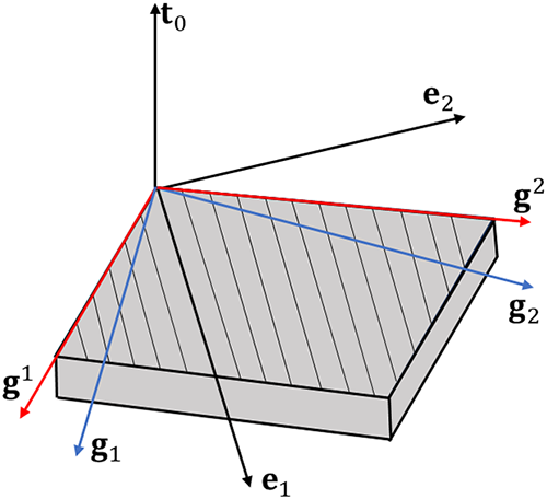
Figure 2: Local coordinate systems for a single layer

Although the current formulations are applied to linear elastic laminates, the HQEM framework can be extended to accommodate more complex scenarios, such as those involving plasticity and functionally graded materials, by introducing appropriate inelastic material models. These extensions will be explored in future work.

3  Rotation Description

In classical shell theory, the individual element nodal variable vector δu is defined as

δu=[δrTδθ1δθ2]T(14)

where δθ1 and δθ2 represent the two rotation components, respectively. The current director t can be obtained through quaternions [42] as

t=q∘e3∘q∗(15)

where q∗ is the conjugated quaternion, and e3=[001]T denotes one of the base vectors of the Cartesian coordinate. The current quaternion q can be updated from the initial quaternion q0 as

q=exp⁡(δθ/2)∘q0(16)

in which

exp⁡(δθ/2)=[cos⁡(‖δθ‖/2)sin⁡(‖δθ‖/2)⋅δθ‖δθ‖](17)

and δθ represents the incremental rotation vector. The quaternion representation adopted here has proven to be a stable and efficient tool for algebraic operations [43], enabling a convenient and robust description of spatial rotations and the corresponding update procedures. Besides the quaternion, other rotation parameterizations, such as updating the rotation vector via the rotation tensor [44,45], are also feasible.

The rotation from the initial director to the current director can also be described by the rotation tensor Λ as

t=Λe3(18)

In classical shell theory, the rotation of the director vector t is constrained to remain within its normal plane (i.e., no drilling rotation). In addition, the director orthogonal frame is denoted by {tα} (α = 1, 2, 3). The {tα} (α = 1, 2, 3) is defined as

tα=Λαeα(α=1,2),t3=Λe3=t(19)

where ei (i=1,2,3) represents the inertial (fixed) basis of the Cartesian reference frame {eα} (α=1,2,3), and defined as

e1=[100]T,e2=[010]T,e3=[001]T(20)

Because the drilling rotation of director t is omitted, the rotations at a point are described by only two independent variables (δθ1 and δθ2). Therefore, the infinitesimal incremental rotation vector δθ is constrained to be orthogonal to t and its variation δt. In this way, the infinitesimal incremental rotation vector δθ can be obtained as

δθ=t×δt=[t1t2][δθ1δθ2](21)

For the orthogonality of the rotation tensor Λ, the variation of Λ is given by introducing a rotation vector variation δθ as

δΛ=δθ^Λ(22)

where ^ denotes the skew-symmetric tensor form of a vector. The variation of t thus can be obtained from Eq. (18) as

δt=δΛt0=−t^δθ=−t^[t1t2][δθ1δθ2](23)

4  Element Formulation of HQEM

4.1 Shape Functions for HQEM

Although the quadrilateral element is the most prevalent and is the main element discussed in this work, triangular elements are advantageous in certain cases, such as for modeling circular/spherical shells, for facilitating mesh generation. Consequently, the shape functions for triangular elements are also addressed in this section. Different from the quadrilateral element method (QEM), where all element nodes serve as integration points, the HQEM instead employs Gauss-Lobatto integration points (mg × ng) for numerical integration. The HQEM permits independent node distribution at the vertices, edges, and interior of each element. Provided that the C0 continuity of the basis functions across element boundaries is guaranteed, this flexibility enables the assembly of elements with varying edge-node configurations and arbitrarily distributed face nodes. This capability enables key features such as local p-refinement and the combination of quadrilateral and triangular elements.

4.1.1 Quadrilateral Elements

The hierarchical quadrature elements with curved edges in two-dimensional domains are shown in Fig. 3. The bases on the edges of the quadrilateral element are Serendipity interpolation shape functions based on non-uniform Gauss-Lobatto nodes, while the bases inside the quadrilateral element are the hierarchical shape functions in tensor product form.

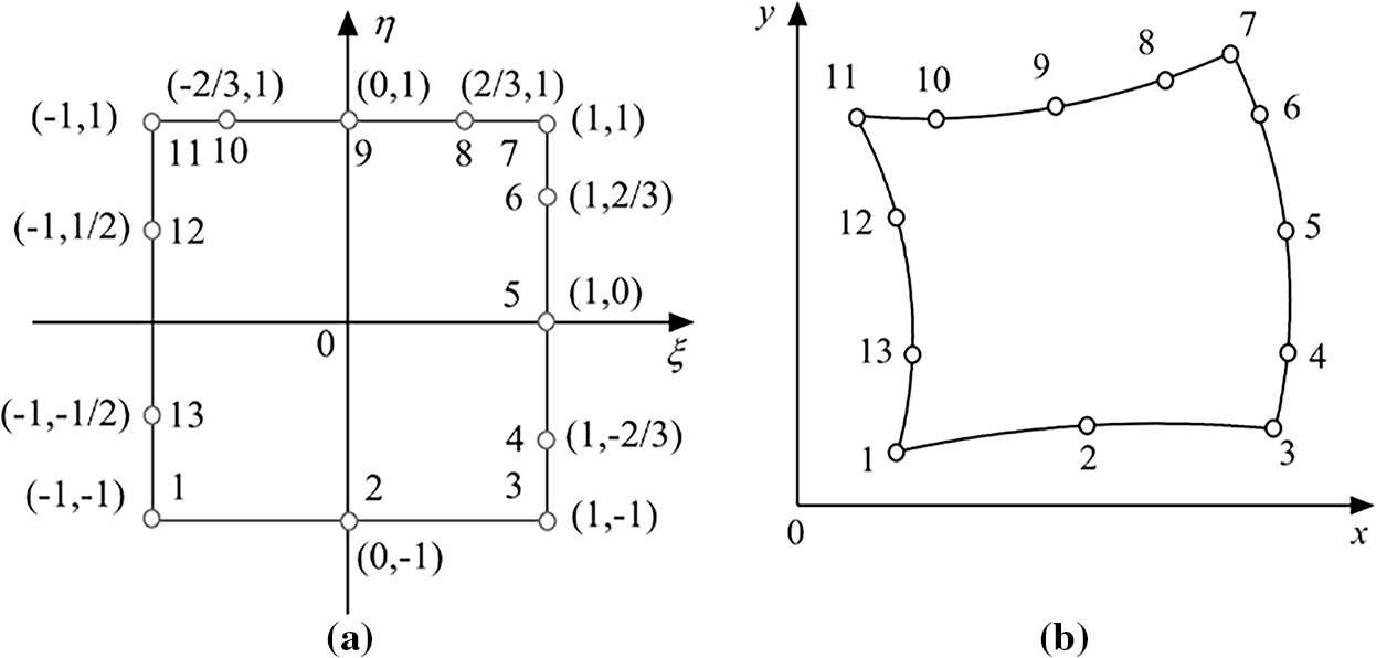
Figure 3: A quadrilateral element: (a) parametric domain, (b) geometric domain

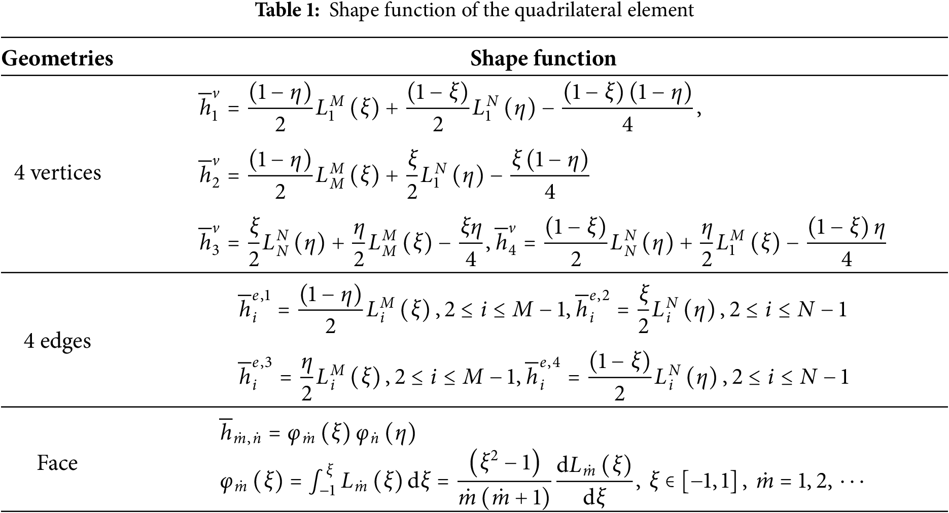
As illustrated in Fig. 3, this flexibility enables varying nodal counts along individual edges in the quadrilateral element. The corresponding shape functions for these geometric features are respectively defined as Table 1. The shape function matrix h¯ are defined as

h¯=[h¯1vh¯ie,1h¯2vh¯ie,2h¯3vh¯ie,3h¯4vh¯ie,4h¯m˙,n˙](24)

with the dimension of 1 × n, and n represents the total number of HQEM nodes. As depicted in Eq. (24), h¯ie,k(k = 1, 2, 3, 4) is the Serendipity interpolation shape functions on the edges, h¯kv(k = 1, 2, 3, 4) is the shape function at four corners, h¯m˙,n˙ represents the shape function inside the quadrilateral element domain. As shown in Table 1, M and N denote the number of nodes on the boundaries in the ξ and η directions, respectively. Correspondingly, m˙ and n˙ represent the number of nodes in the interior of the element along these directions. LiM(ξ) is the Lagrange shape function corresponding to the i-th node on an edge along ξ direction:

LiM(ξ)=∏j=1,j≠iMξ−ξjξi−ξj.(25)

The Lm˙ is the Legendre polynomials, and

φm˙(ξ)=∫−1ξLm˙(ξ)dξ=(ξ2−1)m˙(m˙+1)dLm˙(ξ)dξ,ξ∈[−1,1],m˙=1,2,⋯(26)

In order to analyze HQEM’s capacity of p-refinement, a simply supported plate subjected to a central point load is modeled as illustrated in Fig. 4a. The material and geometrical parameters are defined as follows: Poisson’s ratio υ=0.3, Young’s modulus E = 10.92 × 105, length l = 5, lΔ = 1.2, and thickness h = 0.1. Due to symmetry, only one quarter of the plate is discretized using a 4-element mesh, an assembly of low-order, transition, and high-order elements. The transition element acts as an intermediate component that smoothly bridges the disparity in nodal density between coarse low-order and refined high-order regions, and thus effectively localizes the refinement influence. As shown in Fig. 4b, compared to uniform p-refinement, the local p-refinement approach demonstrates excellent performance while simultaneously reducing computational costs. The difference in CPU time between the element assembly with pl = ph−3 and the element assembly with uniform p-refinement is denoted as ΔtCPU. Fig. 4b additionally plots ΔtCPU against the number of nodes per side of the high-order element. It is noteworthy that locally increasing the element order leads to growth in the condition number of the system matrix. However, our numerical experiments show that, for the same maximum order ph, the condition number of the local p-refinement scheme remains on the same order of magnitude as that of the global uniform refinement scheme. The increase is primarily governed by the local maximum order ph, rather than the order jump (ph−pl).

Figure 4: (a) quadrilateral p-refinement; (b) central point deflection comparing local p-refinement and uniform p-refinement, where ph and pl represent the p-order of high-order and low-order elements

4.1.2 Trilateral Elements

For modeling spherical or circular shells, the use of triangular elements offers a dual advantage in both geometric representation and computational efficiency. First, the triangular element naturally conforms to the rotational symmetry, which simplifies mesh generation; second, under a comparable total number of DOFs, the triangular element typically achieves a higher polynomial order, thereby promoting faster convergence relative to other element types.

The hierarchical trilateral elements with curved edges in two-dimensional domains are shown in Fig. 5. The corresponding shape function matrix h¯ is defined as

h¯=[h¯1vh¯ie,1h¯2vh¯ie,2h¯3vh¯ie,3h¯m˙,n˙](27)

with the dimension of 1 × n. The corresponding shape functions for these geometric features are defined as shown in Table 2. Here, alongside M and N, Q is introduced, which represents the number of nodes on the trilateral element’s 2nd edge. The Jacobi polynomials Pm˙(α,β) are employed to construct the hierarchical shape functions inside the HQEM element. The recursion formula of Jacobi polynomials is as follows

a1iPi+1(α,β)(ξ)=(a2i+a3iξ)Pi(α,β)(ξ)−a4iPi−1(α,β)(ξ)(28)

where i is a nonnegative integer, α > −1, β > −1 and

P0(α,β)(ξ)=1,P1(α,β)(ξ)=12[α−β+(α+β+2)ξ](29)

and

a1i=2(i+1)(i+α+β+1)(2i+α+β)a2i=(2i+α+β+1)(α2−β2)a3i=(2i+α+β)(2i+α+β+1)(2i+α+β+2)a4i=2(i+α)(i+β)(2i+α+β+2)(30)

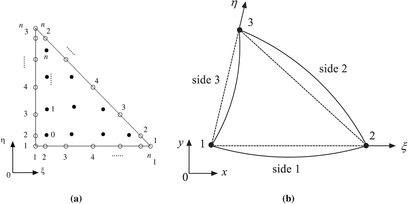
Figure 5: A triangular element: (a) parametric domain, (b) geometric domain

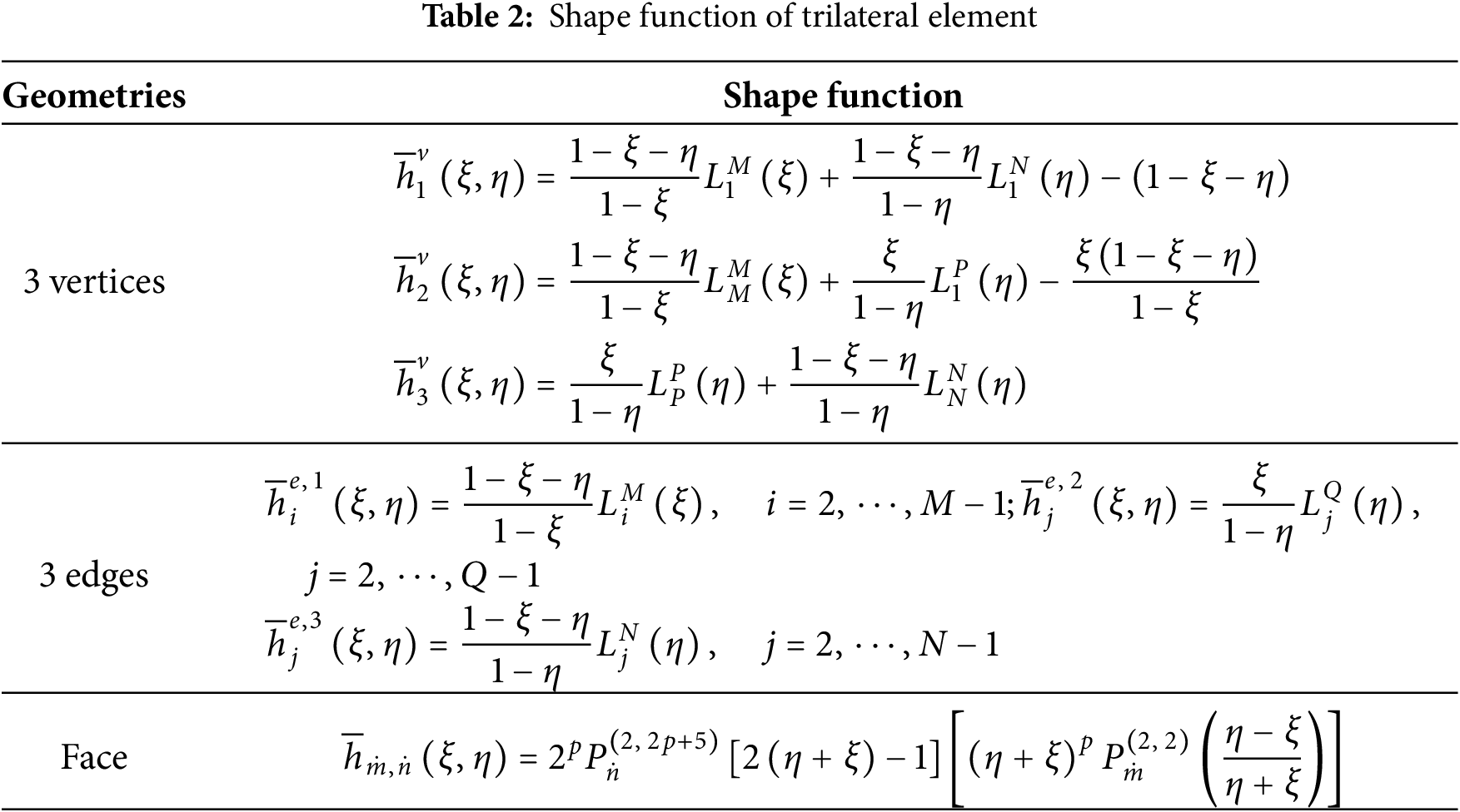
The Jacobi polynomials are defined on [−1, 1].

It is well known that the trilateral element is conveniently applied to modeling circular/spherical shells for facilitating mesh generation. A fully clamped elastic circular plate subjected to a uniform pressure is analyzed in this work, as shown in Fig. 6a. Due to symmetry, a quarter of the plate is modeled using either a single triangular element or a combination of quadrilateral and triangular elements, with all elements having 11 nodes per side. As shown in Fig. 6b, the results from the trilateral HQEM are in excellent agreement with both the analytical solution (Chia et al. [46]) and the reference numerical solution (Wang et al. [47]).

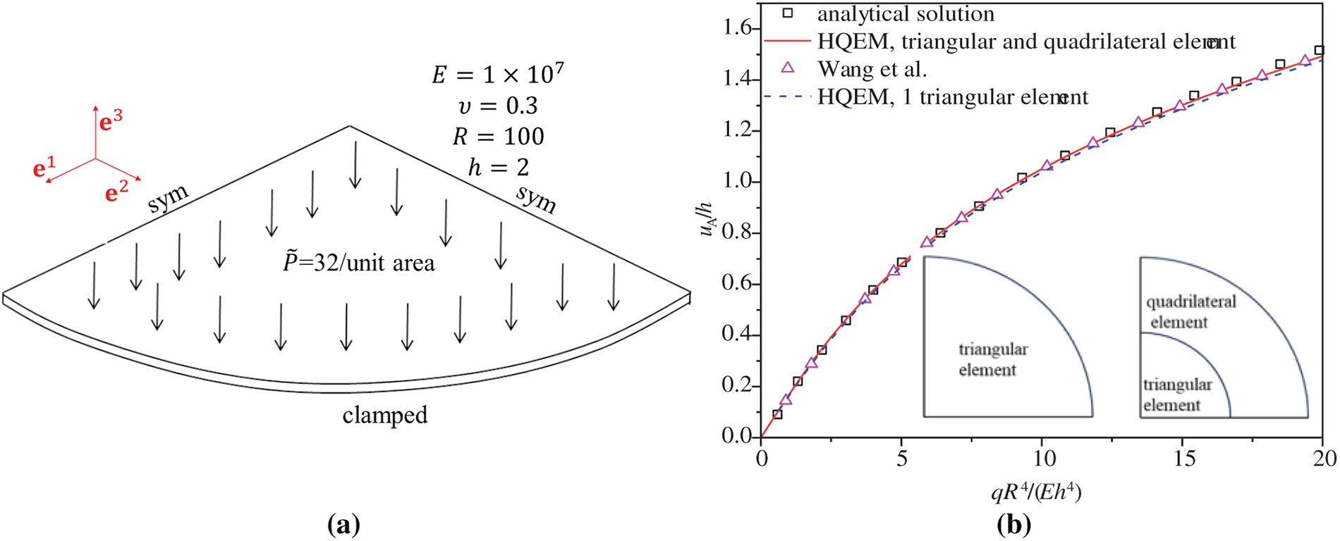
Figure 6: (a) Trilateral p-refinement; (b) normalized central deflection results for the clamped circular plate

4.2 Discretization of Element Virtual Work through the HQEM

Assuming that the number of layers through the thickness of the laminated shell is nl, the element internal virtual work δWint can be written as

δWint=∫V0(e)(s:δϵ)dV0=∫A0(e)∑p=1nl∫x(p)3x(p+1)3j0sijδϵijdx3dx1dx2=∫A0(e)∑p=1nl∑k=01∑l=01(a(k+l)(p)j0δϵ(k)TD(p)ϵ(l))dx1dx2(31)

where x(p+1)3 and x(p)3 represent the thickness coordinates on the upper and the lower surface of the pth layer. As shown in Eq. (31), a(k+l)(p) represents the weighted thickness coefficient of the pth layer, which serves to partition the through-thickness integration term and is obtained as

a(k+l)(p)=∫x(p)3x(p+1)3(x3)(k+l)dx3(32)

with the integer (k + l) ranging from 0 to 2. The weighted thickness coefficients a(k+l)(p) defined in Eq. (32) are evaluated analytically for each layer. For shells with a single layer, Eq. (31) can be written as

δWint=∫A0(e)[j0hδε(0)TDε(0)+112j0h3δε(1)TDε(1)]dx1dx2(33)

The Gauss-Lobatto quadrature [48] is employed to evaluate integrals in the Hierarchical Quadrature Element Method (HQEM), with mg and ng integration points assigned along its two dimensions, respectively. The total nodal variable vector δd for an HQEM element with n nodes are defined as

δd=[δu1T⋯δuiT⋯δunT](34)

the definition of δui can be referred to Eq. (14). And then, the global nodal coordinate array δd is reorganized into five n × 1 consolidated vectors: δr1, δr2, δr3, δθ1, δθ2, each collecting the respective component from all n nodes. This restructuring enhances computational efficiency and facilitates subsequent interpolation processes.

The variation of strain measures at the (i, j) Gauss-Lobatto integration point can now be expressed as:

δεij(k)=Bij(k)δd(k=0,1)(35)

in which

Bij(k)=Aij(k)Hij(k=0,1)(36)

and

Aij(0)=[r,1T01×301×201×401×3r,2T01×201×4r,2Tr,1T01×201×4tT01×3r,1TΛ¯01×401×3tTr,2TΛ¯01×4],Aij(1)=[t,1T01×3r,1TΛ¯,1r,1TΛ¯01×201×3t,2Tr,2TΛ¯,201×2r,2TΛ¯t,2Tt,1Tr,2TΛ¯,1+r,1TΛ¯,2r,2TΛ¯r,1TΛ¯02×302×302×202×202×2],Λ¯=−t^[t1t2](37)

Hij=[h¯,1T0n×10n×1h¯,2T0n×10n×10n×10n×10n×10n×10n×10n×10n×1h¯,1T0n×10n×1h¯,2T0n×10n×10n×10n×10n×10n×10n×10n×10n×1h¯,1T0n×10n×1h¯,2T0n×10n×10n×10n×10n×10n×10n×10n×10n×10n×10n×10n×1h¯T0n×1h¯,1T0n×1h¯,2T0n×10n×10n×10n×10n×10n×10n×10n×1h¯T0n×1h¯,1T0n×1h¯,2T]T(38)

At the integration point (i, j), the partial derivatives r,α, t,α (for α=1,2) are interpolated from the corresponding derivatives of the interpolation shape function h, namely h,1, h,2, which represent the partial derivatives along the two coordinate directions.

Application of Eqs. (33)–(35), the internal force Gint can be obtained as

Gint=∑i=1mg∑j=1ngwiwjj0ij|Jij|∑p=1nl∑k=01∑l=01(a(k+l)(p)Bij(k)TD(p)ε(l))ij(39)

for a single layer, Gint can be obtained as

Gint(e)=∑i=1mg∑j=1ngwiwjj0ij|Jij|[hB(0)TDε(0)+112h3B(1)TDε(1)](40)

The external force Gext can be obtained as

Gext=∑i=1mg∑j=1ngwiwjj0ij|J|ijTijNa(e)+∑p∑i=1mgwiµαipTipNlip(e)+∑q∑j=1ngwiµαqjTqjNlqj(e)+∑TrsNnrs(e)(41)

with

Tij=[⋯δikδjl[I3×303×203×3[t01t02]klT]⋯](42)

Na(e)=[⋯P~klTm~klT⋯],Nl(e)=[⋯P¯klTm¯klT⋯],Nn(e)=[⋯PklTmklT⋯](43)

J=[∂x1∂ξ1∂x1∂ξ2∂x2∂ξ1∂x2∂ξ2]=[J11J12J21J22],|J|=J11J22−J12J21(44)

in which J is the Jacobian matrix, and |J| is the corresponding Jacobian determinant. The vector Gext is determined primarily through the Tij matrix, where the subscript pair (i, j) corresponds to the nodal point at which the external force is applied. This correspondence is implemented numerically by employing the Kronecker delta δij in the assembly process. And then, Gext is reformulated into the vector comprising five n×1 sub-vectors that correspond to δd. P~ and m~ are area force and moment vector, P¯ and m¯ are line force and moment vector, P and m are nodal force and moment vector; t01 and t02 represents the orthonormal basis in initial configuration; μ1=ds/dξ and μ2=ds/dη; the wi and wj denote the weighting coefficients of the Gauss-Lobatto quadrature points along the two respective dimensions.

4.3 Tangent Stiffness Matrix

Suppose that R¯(i) and d(i) are the nodal residual force vector and the nodal displacement vector after the i-th iteration (respectively), with their increments denoted as ΔR¯(i) and Δd(i). For an equilibrium configuration, the incremental form of the residual force is defined as

ΔR¯=KΔd(45)

where K represents the tangent stiffness matrix. The solution is considered convergent if both of the following inequality criteria are satisfied:

‖ΔR¯(i)‖≤τ‖R¯(i)‖ or ‖Δd(i)‖≤τ‖d(i)‖(46)

The tolerance parameter τ is set to a small value, such as 1 × 10−6. The global residual force vector R¯ is given by

R¯=Gint−Gext(47)

According to Eq. (39), where the internal stiffness matrix Kint can be obtained from the variation of internal force Gint as

Kint=∑i=1mg∑j=1ngwiwjj0ij|Jij|∑p=1nl∑k=01∑l=01a(k+l)(p)ij[Bij(k)TD(p)Bij(l)+HijTΞ(p)ij(k+l)Hij+HijTΨ(k+l)Hij](48)

for a single layer, the inner stiffness matrix Kint can be obtained as

Kint=h∑i=1mg∑j=1ngwiwjj0ij|Jij|[Bij(0)TDBij(0)+HijTΞij(0)Hij+HijTΨ(0)Hij]+112h3∑i=1mg∑j=1ngwiwjj0ij|Jij|[Bij(2)TDBij(2)+HijTΞij(2)Hij++HijTΨ(2)Hij](49)

in which

Ξ(0+l)=[s11(l)I3×3s12(l)I3×3s13(l)Λ¯03×4s12(l)I3×3s22(l)I3×3s23(l)Λ¯03×4s13(l)Λ¯Ts23(l)Λ¯T02×202×404×304×304×204×4](50)

Ξ(1+l)=[03×303×3s11(l)Λ¯,1+s12(l)Λ¯,2s11(l)Λ¯s12(l)Λ¯03×303×3s12(l)Λ¯,1+s22(l)Λ¯,2s12(l)Λ¯s22(l)Λ¯s11(l)Λ¯,1T+s12(l)Λ¯,2Ts12(l)Λ¯,1T+s22(l)Λ¯,2T02×202×202×2s11(l)Λ¯Ts12(l)Λ¯T02×202×202×2s12(l)Λ¯Ts22(l)Λ¯T02×202×202×2](51)

Ψ(0+l)=[06×606×206×402×6−[t1Tt2T](s13(l)r^,1+s23(l)r^,2)Λ¯02×404×604×204×4](52)

Ψ(1+l)=[06×606×206×206×202×6−[t1Tt2T][(s11(l)r^,1+s12(l)r^,2)Λ¯,1+(s22(l)r^,2+s12(l)r^,1)Λ¯,2]−[t1Tt2T](s11(l)r^,1+s12(l)r^,2)Λ¯−[t1Tt2T](s22(l)r^,2+s12(l)r^,1)Λ¯02×6−[t1Tt2T](s11(l)r^,1+s12(l)r^,2)Λ¯02×202×202×6−[t1Tt2T](s22(l)r^,2+s12(l)r^,1)Λ¯02×202×2](53)

where Λ¯,1 and Λ¯,2 are the partial derivatives of Λ¯ along the two coordinate directions at the integration point (i, j), and are obtained via interpolation of the corresponding shape function derivatives, h,1 and h,2.

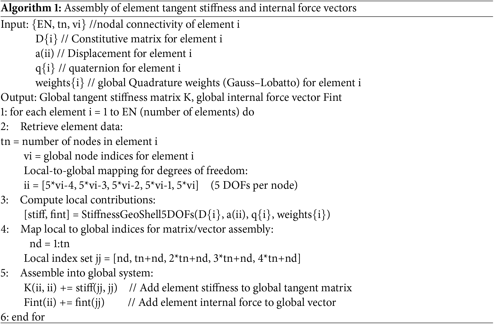
Fig. 7 presents the flowchart of the simulation process, with several critical steps highlighted: Node sampling automatically distributes nodes based on inter-node distances while assigning identical numbers to nodes sharing coordinates (step 3); Stiffness matrices and force vectors are computed through Eqs. (39)–(53) (step 4); The nonlinear system in Eq. (45) is solved using either Newton-Raphson (Sections 5.1–5.3) or arc-length methods (Sections 5.4–5.7) (step 7); Solution accuracy is enhanced through local or global p-refinement (step 9); and final mode shapes or deformation patterns are visualized using integration nodes with Gauss-Lobatto quadrature, which provides numerical advantages over standard Gauss quadrature (step 10). The pseudocode for the key steps of element matrix assembly is provided in Algorithm 1. This procedure is applicable to both global and local p refinement, wherein the element stiffness matrix and internal force vector are computed through the weighting coefficients of the Gauss–Lobatto quadrature points.

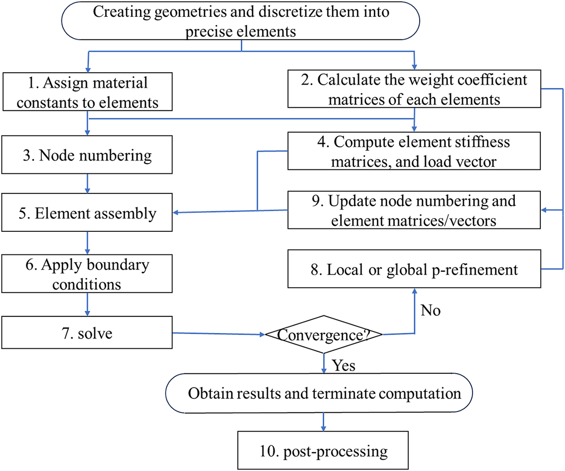
Figure 7: Flow chart of the simulation process by the HQEM

5  Numerical Examples

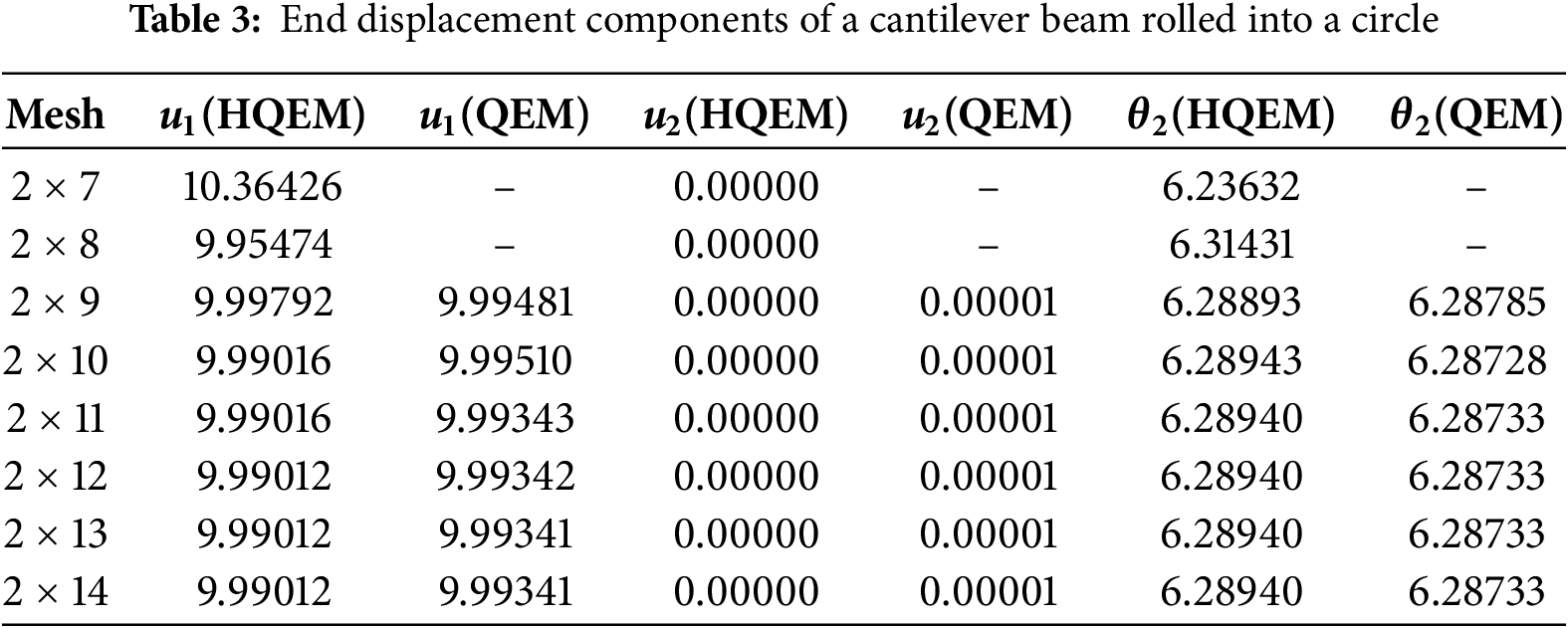
5.1 Cantilever Beam under a Tip Moment

This example analyzes a cantilever beam under a prescribed drilling rotation at its free end—a classical benchmark for large deformation analysis. As shown in Fig. 8, the material parameters are defined as follows: Poisson’s ratio υ=0, length l = 10, width w = 1, and thickness h = 0.1, and Young’s modulus E = 1.2 × 107. The beam is subjected to a line moment m¯=200π per unit length at its tip and is modeled using a single HQEM element. The load is applied incrementally in four steps. Fig. 9 illustrates the initial and deformed configurations at each load step in the e1–e3 plane using a single HQEM element of 2 × 13 nodes. It’s observed by Xiao and Zhong [49], many beam formulations experience membrane locking and fail to accurately capture deformations when the beam bends into a semicircle. In contrast, the present method successfully forms a full circle in only 4 load steps, demonstrating its robustness in handling large load increments. With the tolerance parameter τ set to 1 × 10−6, Table 3 summarizes the displacement components u at the free end for the last load step. By leveraging high-order approximation, HQEM inherently mitigates shear and membrane locking. As shown in Table 3, the minimum number of nodes along the length needed for a full circular roll-up is 7. The results show that displacements converge as the number of integration nodes along the length increases, demonstrating that HQEM’s high-order basis is crucial for accurately capturing the circular configuration. Furthermore, the HQEM results align closely with those from the weak-form quadrilateral element method (QEM) by Zhang et al. [9], confirming that HQEM achieves quantitatively comparable accuracy and efficiency to QEM. It is also worth noting that while the final configuration from QEM exhibits a slight out-of-plane deviation u2(QEM) = 0.00001 along the e2-direction, the HQEM result shows virtually no deviation, with u2(HQEM) = 0.00000, further validating its superior numerical reliability.

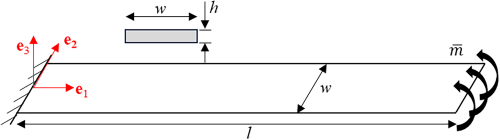
Figure 8: Roll-up of a cantilever beam

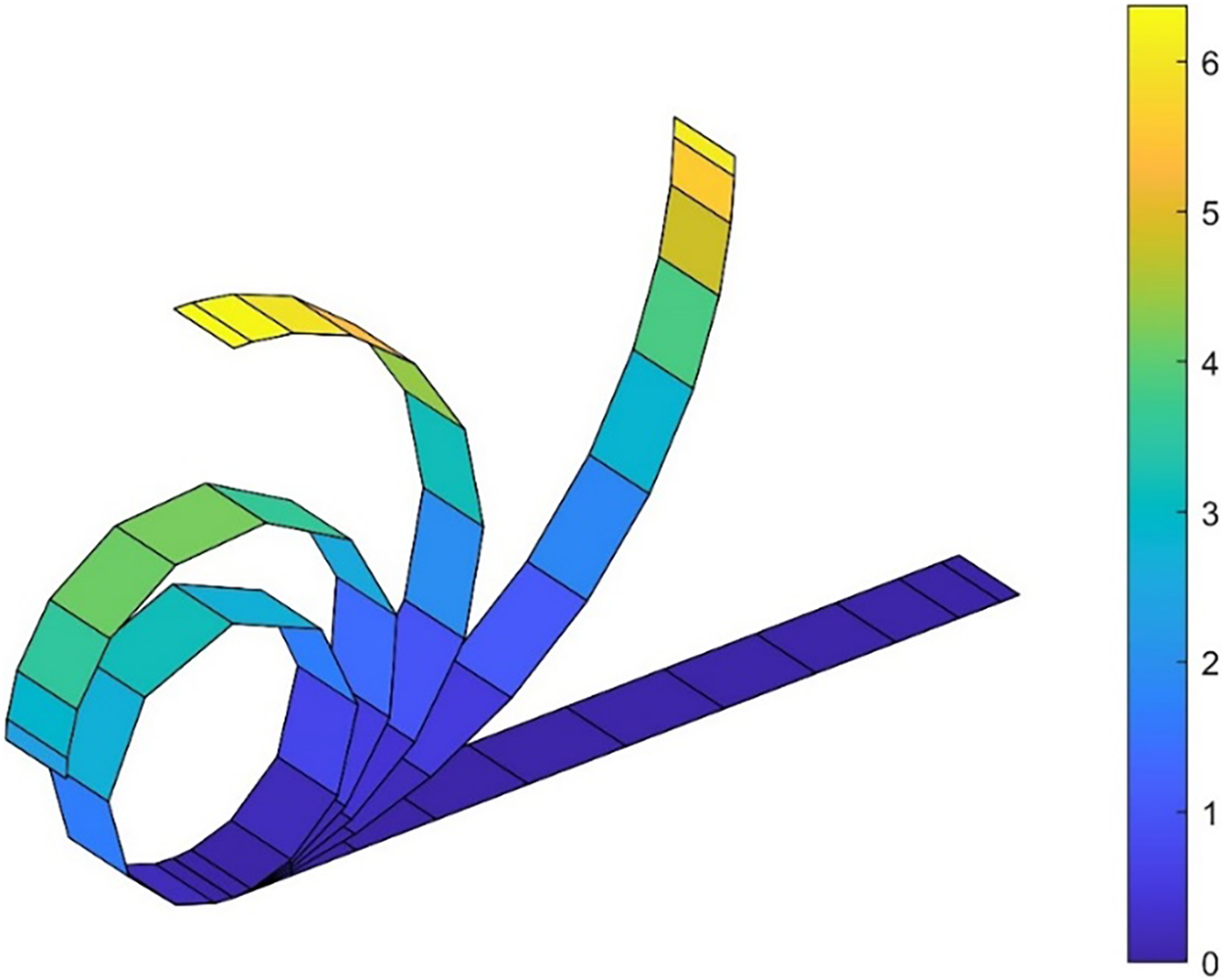
Figure 9: Initial and deformed configurations of a cantilever beam subjected to an end moment

5.2 Ring Plate Loaded at Free Edge

In this section, a ring plate under a free-edge load is analyzed to assess the HQEM’s capabilities in avoiding shear locking. It is acknowledged that low-order shape functions tend to artificially stiffen the element, resulting in severely underestimated displacements, a phenomenon known as shear locking. By leveraging high-order approximation, HQEM inherently mitigates shear and membrane locking. Fig. 10a illustrates a ring plate that is clamped along its inner edge and subjected to a line force of P¯ = 6000 per unit length along the free outer edge. The geometric and material parameters are as follows: inner radius R1 = 6, outer radius R2 = 10, thickness h = 0.03, Young’s modulus E = 2.1 × 1011, and Poisson’s ratio υ = 0. The plate is modeled using a single quadrilateral element with 14 × 7 nodes in the circumferential and radial directions, respectively. Fig. 10b plots the vertical displacements at points A, B against the applied load, together with the final deformed configuration. The results from the present formulation show excellent agreement with those of Büechter and Ramm [50] obtained using a 16 × 2 mesh of 16-node degenerated shell elements, thereby validating the proposed model.

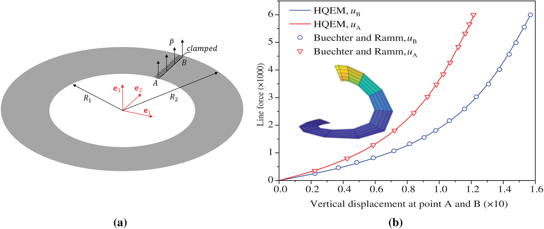
Figure 10: (a) Ring plate loaded at free edge; (b) deflection–load curves for a ring plate loaded at free edge

5.3 Pinched Hemispherical Shell with 18° Hole

This test is widely used to evaluate a formulation’s capability in handling rigid body modes, inextensional bending, and membrane locking [51]. As shown in Fig. 11a, a hemispherical shell with an 18° polar cutout is subjected to alternating radial forces P. The structure, with radius R = 10, thickness h = 0.04, cutout angle θ¯ = 18° is modeled using one quadrant due to symmetry. For isotropic case, the material parameters are Young’s modulus E = 6.825 × 107, and Poisson’s ratio υ = 0.3. As shown in Fig. 11b, the radial displacements at points A and B under the applied load, obtained with a 12 × 12 nodes, agree excellently with the reference solution from Büechter and Ramm [51] based on 256 four-node assumed-strain elements. In addition to isotropic materials, two anisotropy laminate configurations are examined. The first is a [45°/0°/−45°] laminate with uniformly thick layers. The second is a [30°/0°] laminate, where the 30° ply has a thickness of 0.75h and the 0° ply a thickness of 0.25h. For the anisotropic case, the material properties are: E1 = 7 × 107, E2 = E3 = 7 × 106, G12 = G13 = 7 × 107, G23 = 1 × 107, and υ12 = υ13 = υ23 = 0.3. As shown in Fig. 11c, the results exhibit excellent agreement with those obtained by Abaqus S4 element (25 × 25 elements), confirming the accuracy of the present method in modeling nonlinear behavior for anisotropy laminated composite shells.

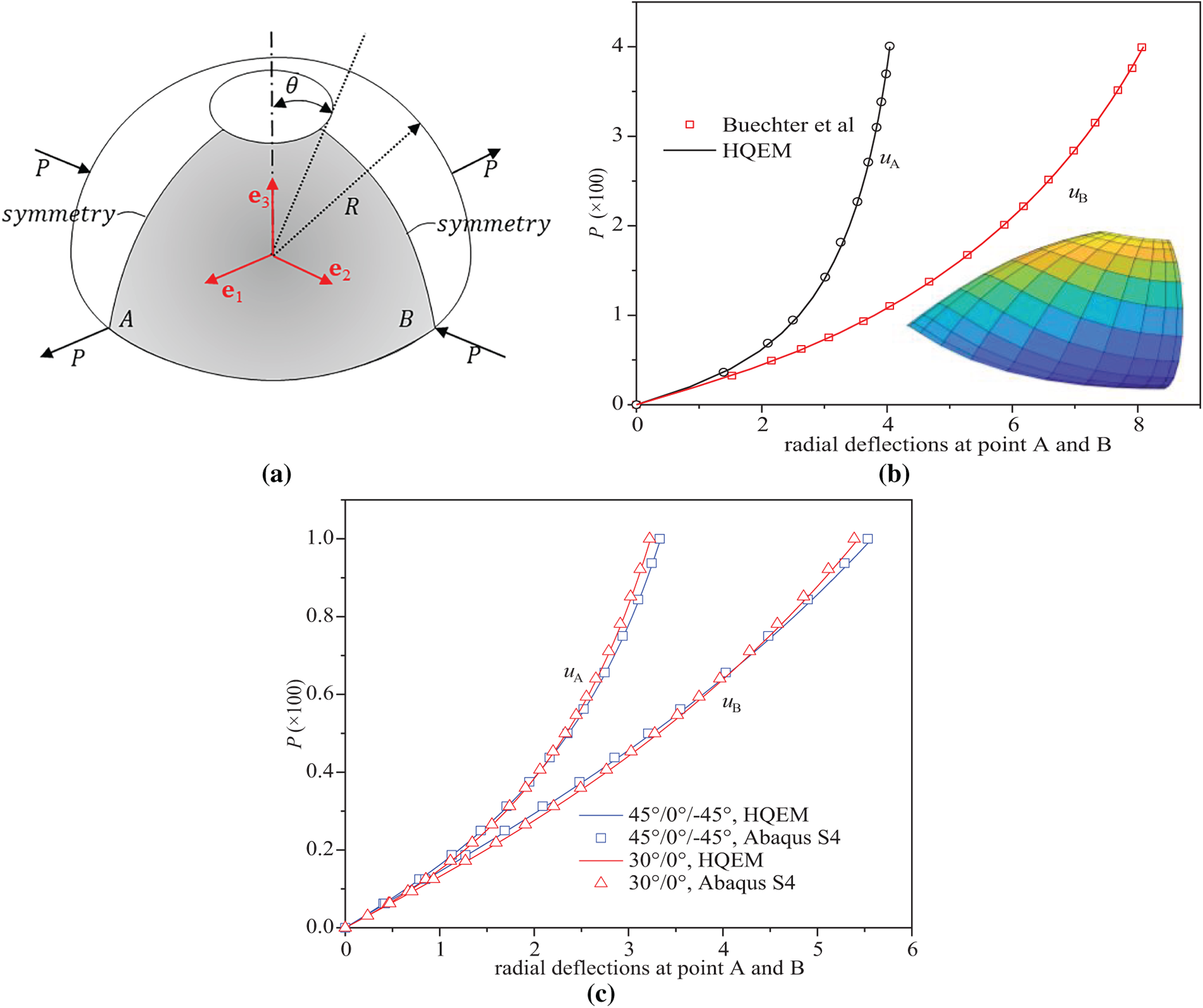
Figure 11: (a) Pinched hemispherical shell with 18° hole; (b) displacement–load curves for pinched hemispherical shell; (c) deflection–load curves for hemispherical laminate shell

5.4 Stretch and Compression of a Cylindrical Shell with Free Edge

This study investigates a free-ended cylindrical shell under opposing radial forces (tensile or compressive). This problem is a recognized benchmark in nonlinear shell analysis because its boundary conditions can induce hourglass modes with the use of reduced integration [9]. As shown in Figs. 12a and 13a, the shell has a length l = 10.35, radius R = 4.953, and thickness h = 0.094, with a Young’s modulus of E = 10.5 × 106 and Poisson’s ratio υ = 0.3125. Leveraging symmetry, one-eighth of the shell is modeled. A single quadrilateral element with 10 × 17 nodes was used to analyze the stretching of this cylindrical shell. Under tensile loading (P from 0 to 40,000), Fig. 12b plots the radial deflections at points A, B, and C. The response features two distinct regions separated by a snap-through buckling stage, characterized by one stable configuration to another. The spherical arc-length method was employed to trace this stiff response and capture the buckling behavior [52] by adjusting load increments dynamically based on the current state. With a single quadrilateral element, a clear snap-through phenomenon is only observed when the number of nodes along the perimeter is at least 9 and along the radius is at least 5. Notably, the curves become significantly steeper in the post-buckling phase, indicating a sharp increase in structural stiffness. The results agree excellently with the numerical simulation obtained by Ota et al. [53]. For the compression case (P from 0 to 2900), the cylindrical shell was analyzed using a single quadrilateral element with 12 × 12 nodes. Fig. 13b presents the load-deflection curves at points A and B; the response at point C closely follows that of point B and is omitted for clarity. The present results show excellent agreement with the reference solution of Zhang et al. [9] obtained using the quadrilateral element method (QEM) with a 12 × 12 nodal configuration, demonstrating that the HQEM achieves quantitatively comparable accuracy to QEM. In addition, a 9-element mesh, consisting of low-order, transition, and high-order elements, discretizes one-eighth of the cylinder for the compression case (P = 3000), as illustrated in Fig. 13c. As shown in Fig. 13d, selecting a suitable local p-refinement strategy can achieve high accuracy and reduced computational cost relative to uniform p-refinement.

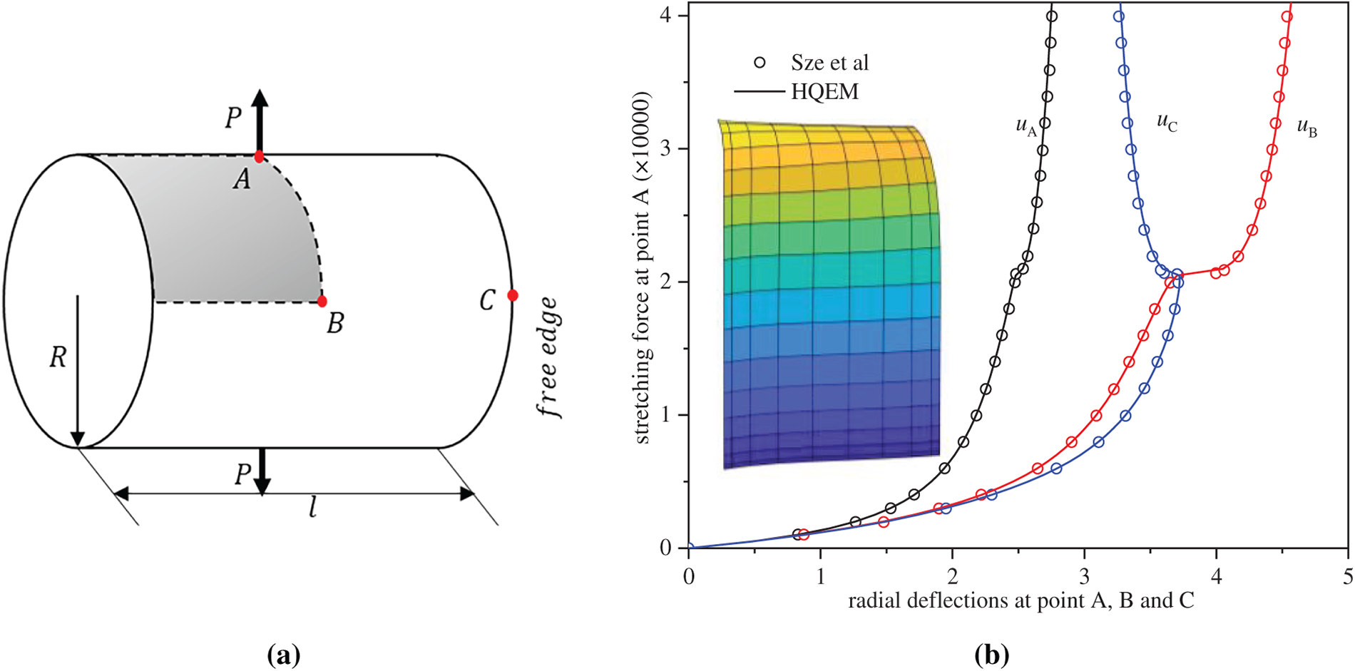
Figure 12: (a) Stretch of a cylindrical shell with free end; (b) deflection–load curves of a cylindrical shell subjected to stretch

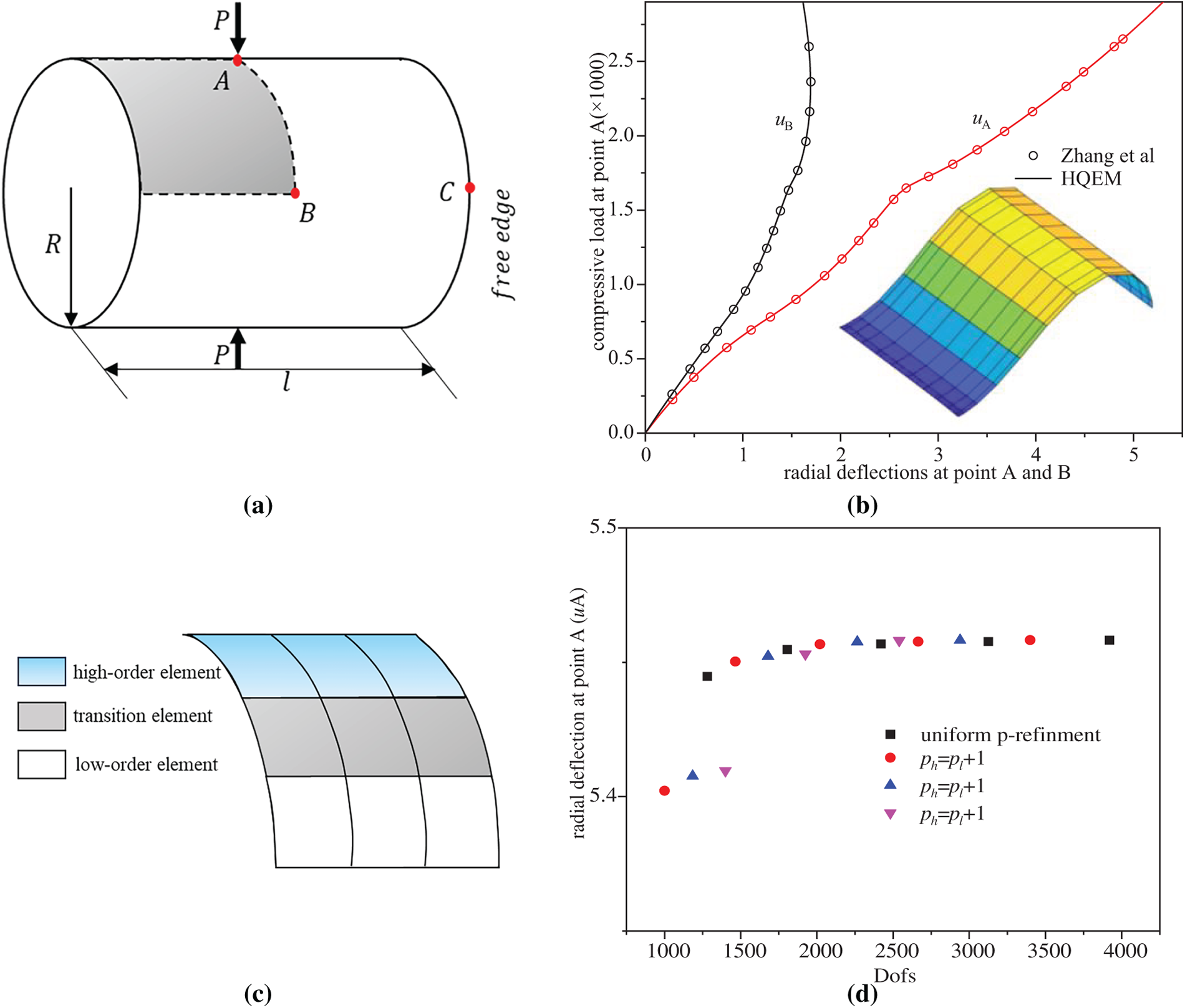
Figure 13: (a) Compression of a cylindrical shell with free end; (b) deflection–load curves of a cylindrical shell subjected to compression; (c) local p-refinement strategy discretizing one-eighth of the cylinder; (d) radial deflection of point A comparing local p-refinement and uniform p-refinement

5.5 Pinched Semi-Cylindrical Shells

This section analyzes a semi-cylindrical shell subjected to a pinching force at the midpoint of its free-hanging circumferential edge, which has been analyzed by various researchers [54–56]. The opposite edge is fully clamped, while both longitudinal edges are restrained in vertical deflection and rotation about the e2-axis. As shown in Fig. 14a, the geometric properties are as follows: radius R = 101.6, length l = 304.8, thickness h = 3. For the isotropic case, the material parameters are Young’s modulus E = 2068.5, and Poisson’s ratio υ = 0.3. For the anisotropy case, laminates with stacking sequences [0°/90°/0°] and [90°/0°/90°] are considered. The anisotropy material parameters are E1 = 2068.5, E2 = E3 = 517.125, G12 = G13 = 795.6, G23 = 198.894, υ12 = υ13 = υ23 = 0.3 for the laminate case. In the laminated shell, all plies are equal in thickness. A ply is of 0° if its fibers are parallel to the longitudinal direction of the shell. In this work, this benchmark problem is simulated using a half-model exploiting symmetry and discretized with a 25 × 16 HQEM mesh. As shown in Fig. 14b, the present HQEM results at point A are in good agreement with the reference data from Sze et al. [57], thus confirming the method’s accuracy in modeling nonlinear behavior for both isotropic and laminated structures.

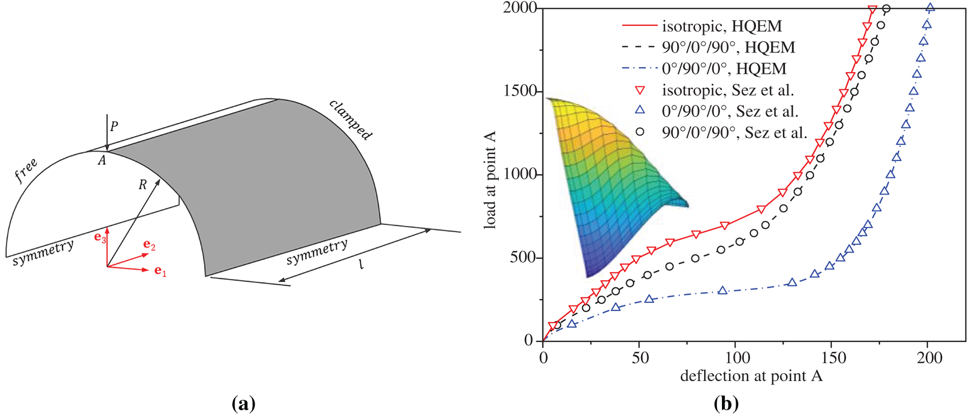
Figure 14: (a) The semi-cylindrical shell subjected to an end pinching force; (b) load–deflection curves of the semi-cylindrical shell subjected to end pinching force

5.6 Hinged Cylindrical Panel with Central Point Load

This example analyzes a hinged cylindrical panel under a central point load, a benchmark problem renowned for its complex snap-back behavior. As shown in Fig. 15a, the panel, defined by a central angle 2θ¯ = 0.2 radians, length l = 508, and radius R = 2540. Due to symmetry, only one quadrant of the panel is modeled using a single quadrilateral HQEM element with 12 × 12 nodes, and two thicknesses are considered: h = 12.7 and h = 6.35. For the isotropic case, the material parameters are Young’s modulus E = 3102.75 and Poisson’s ratio υ = 0.3. Besides isotropic materials, the [0°/90°/0°] laminate and [90°/0°/90°] laminate at two different thicknesses are considered. For the anisotropy case, the material parameters are E1 = 3300, E2 = E3 = 1100, G12 = G13 = 660, G23 = 440, υ12 = υ13 = υ23 = 0.25. The cylindrical arc-length method is employed to trace the nonlinear load-displacement response at the center point [52]. As shown in Fig. 15b–d, the results exhibit excellent agreement with those of Ota et al. [53], confirming the accuracy of the present method in capturing the snap-through response for both isotropic and laminated composite shells.

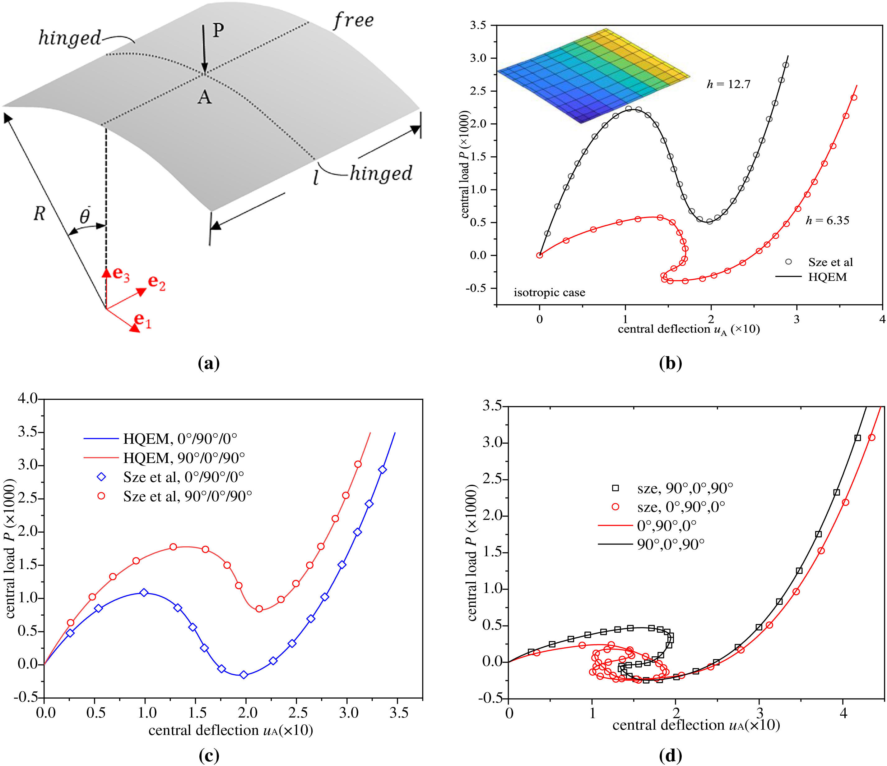
Figure 15: (a) Hinged cylindrical panel with central point load; (b) deflection–load curves of isotropic case for h = 12.7 and h = 6.35; (c) deflection–load curves of laminate case for h = 12.7; (d) deflection–load curves of laminate case for h = 6.35

5.7 Lateral Buckling of a Cantilever Right-Angle Frame

This section demonstrates the ability of the HQEM to predict critical loads and trace complex post-buckling paths by analyzing a right-angle cantilever frame under a concentrated tip load. This structure is prone to lateral buckling beyond a critical load and has been studied using both beam [58–60] and shell [41,61] theories. As shown in Fig. 16a, the frame has dimensions of 240 in length, 30 in width, and 0.6 in height. Its Young’s modulus is 71,240, and its Poisson’s ratio is 0.31. In Case I, the concentrated load is directed outward in-plane along the e3 direction, while in Case II, it is directed inward. To trigger lateral buckling, a perturbation out-of-plane load Pf = 0.0001 is applied. The load-displacement curves at points A and B, obtained with two 13 × 9 HQEM elements, are presented in Fig. 16b. Notably, for the inward loading case (Case II), the QEM [9] (modeled with 2 elements of 13 × 9 nodes) shows marked deviations from the reference results [62] (modeled with 44 9-node CAM elements [61]) at higher loads, and the latter account for drilling rotations and thickness-direction extensions. The maximum relative difference between the two methods is about 9.5%. In contrast, using the identical mesh (two 13 × 9 elements) as the QEM [9], the HQEM—which only considers five variables—maintains excellent agreement with results obtained by Smoleński [62] and Abaqus (120 × 8 × 1 C3D8I solid elements). The enhanced convergence performance of HQEM is attributed to its consistent use of a complete nodal representation for interpolation at integration points. In contrast, the QEM relies on a direction-dependent node selection strategy, which can introduce interpolation inconsistencies. This fundamental difference allows HQEM to more accurately capture the non-uniform deformation gradients and complex nonlinear behavior, thereby achieving better convergence performance. As a result, HQEM demonstrates superior capability in simulating nonlinear structural behavior. Additionally, Fig. 17a,b respectively depict the deformation geometries for Case I and Case II under the concentrated loads (P = 8) by the HQEM (modeled with 2 elements of 13 × 9 nodes). The prediction of the deflection-load curve for a right-angled beam demonstrates that the proposed nonlinear HQEM enables accurate forecasting of buckling instability, which is crucial for the safe design of such structures.

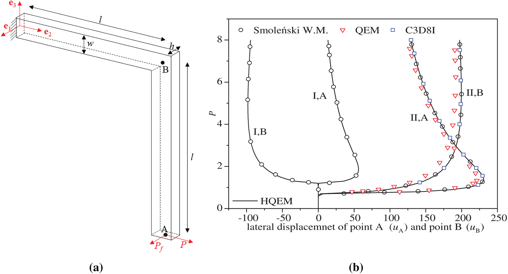
Figure 16: (a) Cantilever right-angle frame under tip load; (b) load–displacement curves for right-angle frame under tip load obtained by HQEM

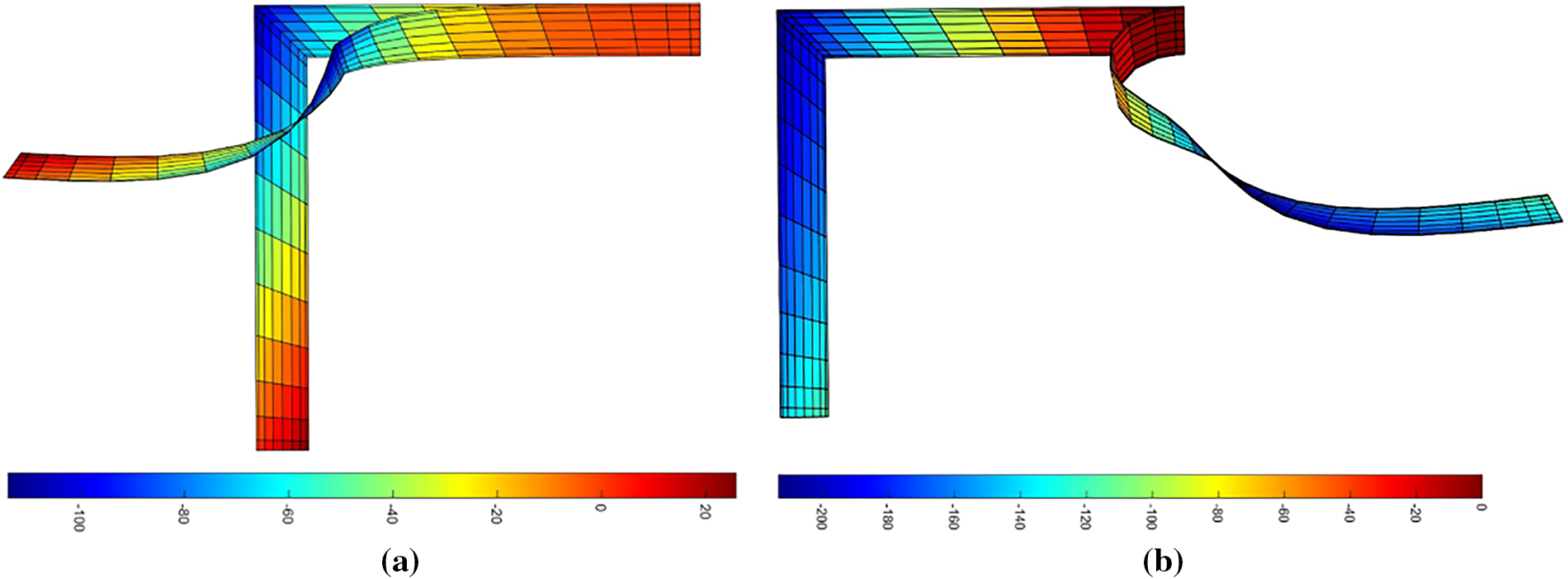
Figure 17: (a) Deformed configurations of the right-angle cantilever under the tip load (P = 8) for (a) Case I and (b) Case II

6  Conclusions

This study presents a unified Hierarchical Quadrature Element Method (HQEM) formulation for the geometrically nonlinear analysis of both isotropic and laminated shells, marking the first implementation of HQEM in nonlinear shell analysis for composite shells. The key innovations and conclusions include: (1) a unified HQEM formulation for geometrically exact isotropic and laminated shells; (2) significant simplification of residual force and stiffness matrix computations; (3) inherent mitigation of shear and membrane locking; (4) convenient support for local p-refinement; (5) compared with the weak-form quadrilateral element (QEM) approach, accurate capture of nonlinear behavior under high loads; and (6) flexible mesh generation through the combination of quadrilateral and triangular elements.

Nevertheless, it is important to acknowledge certain limitations inherent to the current formulation. While classical shell theory remains widely used in engineering practice owing to its lower implementation complexity and computational cost, its exclusion of drilling rotations introduces fundamental limitations in modelling complex geometries, including: the challenges in applying conjugate drilling loads for moment equilibrium; rotational incompatibility at non-smooth shell junctions; and numerical instabilities when handling twisting moment transfer. Furthermore, the HQEM leverages high-order approximation to overcome the high computational costs and locking limitations of low-order elements, yet it introduces new challenges such as meshing difficulties for complex geometries and growth in the condition number, which may pose obstacles to practical application.

Notwithstanding these limitations, the present HQEM formulation establishes a general framework for geometrically exact shell analysis. Although the current formulations are applied to linear elastic laminates, the HQEM framework can be extended to accommodate more complex scenarios, such as those involving plasticity and functionally graded materials, by introducing appropriate inelastic material models. In particular, our subsequent work will focus on: (1) extending the method to the nonlinear analysis of shells incorporating drilling rotation and thickness stretch; (2) implementing inelastic material models for plasticity and functionally graded materials; and (3) undertaking the dynamic analysis of shell structures.

Acknowledgement: None.

Funding Statement: This study is supported by the National Natural Science Foundation of China (Grant Nos. 12472194, 12002018, 11972004, 11772031, 11402015).

Author Contributions: The authors confirm contribution to the paper as follows: Conceptualization and methodology: Bo Liu; software and validation: Yingying Lan; writing—original draft preparation: Yingying Lan; writing—review and editing: Bo Liu. All authors reviewed and approved the final version of the manuscript.

Availability of Data and Materials: The authors confirm that the data supporting the findings of this study are available within the article.

Ethics Approval: Not applicable.

Conflicts of Interest: The authors declare no conflicts of interest.

Nomenclature

References

1. Palazotto AN, Dennis ST. Nonlinear analysis of shell structures. Reston, FL, USA: AIAA; 1992. [Google Scholar]
2. Rebel G. Finite rotation shell theory including drill rotations and its finite element implementation. Delft, The Netherland: Delft University Press; 1998. [Google Scholar]
3. Simo JC, Fox DD. On a stress resultant geometrically exact shell model. Part I: formulation and optimal parametrization. Comput Methods Appl Mech Eng. 1989;72(3):267–304. doi:10.1016/0045-7825(89)90002-9. [Google Scholar] [CrossRef]
4. Naghdi PM. The theory of shells and plates. In: Truesdell C, editors. Linear theories of elasticity and thermoelasticity: linear and nonlinear theories of rods, plates, and shells. Heidelberg, Germany: Springer; 1973. p. 425–640. doi:10.1007/978-3-662-39776-3. [Google Scholar] [CrossRef]
5. Simo J, Fox D, Rifai M. On a stress resultant geometrically exact shell model. Part II: the linear theory; computational aspects. Comput Methods Appl Mech Eng. 1989;73(1):53–92. doi:10.1016/0045-7825(89)90098-4. [Google Scholar] [CrossRef]
6. Ibrahimbegovic A, Brank B, Courtois P. Stress resultant geometrically exact form of classical shell model and vector-like parameterization of constrained finite rotations. Int J Numer Methods Eng. 2001;52(11):1235–52. doi:10.1002/nme.247. [Google Scholar] [CrossRef]
7. Zhang Q, Li S, Zhang A-M, Peng Y. On nonlocal geometrically exact shell theory and modeling fracture in shell structures. Comput Methods Appl Mech Eng. 2021;386:114074. doi:10.1016/j.cma.2021.114074. [Google Scholar] [CrossRef]
8. Ma R, Sun W, Guo T. Phase-field model for ductile fracture in the stress resultant geometrically exact shell. Int J Numer Methods Eng. 2024;125(13):e7462. doi:10.1002/nme.7462. [Google Scholar] [CrossRef]
9. Zhang R, Zhong H. Weak form quadrature element analysis of geometrically exact shells. Int J Non-Linear Mech. 2015;71:63–71. doi:10.1016/j.ijnonlinmec.2015.01.010. [Google Scholar] [CrossRef]
10. Lavrenčič M, Brank B. Hybrid-mixed low-order finite elements for geometrically exact shell models: overview and comparison. Arch Comput Methods Eng. 2021;28(5):3917–51. doi:10.1007/s11831-021-09537-2. [Google Scholar] [CrossRef]
11. Kim M-G, Lee G-H, Lee H, Koo B. Isogeometric analysis for geometrically exact shell elements using Bézier extraction of NURBS with assumed natural strain method. Thin-Walled Struct. 2022;172:108846. doi:10.1016/j.tws.2021.108846. [Google Scholar] [CrossRef]
12. Silva LE, Burgos RB. Second-order two-cycle analysis of frames based on interpolation functions from the solution of the beam-column differential equation. REM-Int Eng J. 2023;76(2):139–46. doi:10.1590/0370-44672022760047. [Google Scholar] [CrossRef]
13. Carrera E, Azzara R, Daneshkhah E, Pagani A, Wu B. Buckling and post-buckling of anisotropic flat panels subjected to axial and shear in-plane loadings accounting for classical and refined structural and nonlinear theories. Int J Non-Linear Mech. 2021;133:103716. doi:10.1016/j.ijnonlinmec.2021.103716. [Google Scholar] [CrossRef]
14. Mallek H, Jrad H, Wali M, Dammak F. Nonlinear dynamic analysis of piezoelectric-bonded FG-CNTR composite structures using an improved FSDT theory. Eng Comput. 2021;37(2):1389–407. doi:10.1007/s00366-019-00891-1. [Google Scholar] [CrossRef]
15. Peres N, Gonçalves R, Camotim D. A geometrically exact beam finite element for curved thin-walled bars with deformable cross-section. Comput Methods Appl Mech Eng. 2021;381:113804. doi:10.1016/j.cma.2021.113804. [Google Scholar] [CrossRef]
16. Garcia-Contreras G, Córcoles J, Ruiz-Cruz JA. Degeneracy-discriminating modal FEM computation in higher order rotationally symmetric waveguides. IEEE Trans Antennas Propag. 2021;69(11):8003–8. doi:10.1109/TAP.2021.3083790. [Google Scholar] [CrossRef]
17. Wang J. Nonlinear finite element based contact modeling for bolted joints in composite laminates. In: Proceedings of the ASME 2021 International Design Engineering Technical Conferences and Computers and Information in Engineering Conference; 2021 August 17–19; Virtual, Online. [Google Scholar]
18. Ibrahimbegovic A, Mejia-Nava RA, Ljukovac S. Reduced model for fracture of geometrically exact planar beam: non-local variational formulation, ED-FEM approximation and operator split solution. Int J Numer Methods Eng. 2024;125(1):e7369. doi:10.1002/nme.7369. [Google Scholar] [CrossRef]
19. Breitenberger M, Apostolatos A, Philipp B, Wüchner R, Bletzinger K-U. Analysis in computer aided design: nonlinear isogeometric B-Rep analysis of shell structures. Comput Methods Appl Mech Eng. 2015;284:401–57. doi:10.1016/j.cma.2014.09.033. [Google Scholar] [CrossRef]
20. Zhang Z, Sun C. Structural damage identification via physics-guided machine learning: a methodology integrating pattern recognition with finite element model updating. Struct Health Monit. 2021;20(4):1675–88. doi:10.1177/1475921720927488. [Google Scholar] [CrossRef]
21. Gassler L, Afrasiabi M, Bambach M. Efficient process simulation of metallic bipolar plate stamping using a GPU-accelerated one-step solver. J Manuf Process. 2024;131(1):2491–504. doi:10.1016/j.jmapro.2024.09.118. [Google Scholar] [CrossRef]
22. Bartezzaghi A, Cremonesi M, Parolini N, Perego U. An explicit dynamics GPU structural solver for thin shell finite elements. Comput Struct. 2015;154:29–40. doi:10.1016/j.compstruc.2015.03.005. [Google Scholar] [CrossRef]
23. Zienkiewicz OC, Gago JDS, Kelly DW. The hierarchical concept in finite element analysis. Comput Struct. 1983;16(1–4):53–65. doi:10.1016/0045-7949(83)90147-5. [Google Scholar] [CrossRef]
24. Phung-Van P, Hung P, Tangaramvong S, Nguyen-Xuan H, Thai CH. A novel Chebyshev-based both meshfree method and shear deformation theory for functionally graded triply periodic minimal surface flat plates. Comput Struct. 2025;309(1):107660. doi:10.1016/j.compstruc.2025.107660. [Google Scholar] [CrossRef]
25. Hung P, Thai CH, Phung-Van P. A novel meshfree method for free vibration behavior of the functionally graded carbon nanotube-reinforced composite plates using a new shear deformation theory. Comput Math Appl. 2025;189:208–24. doi:10.1016/j.camwa.2025.04.023. [Google Scholar] [CrossRef]
26. Li X, Huang C, Zhao S, Qiu S, Liu W, Chen J, et al. A weak-form quadrature element method for modal analysis of electric motor stators. Mech Syst Signal Process. 2025;228:112380. doi:10.1016/j.ymssp.2025.112380. [Google Scholar] [CrossRef]
27. Mo S, Liu J, Zhang R, Yao X. A geometrically exact higher-order shell model for functionally graded materials and its weak form quadrature element formulation. Thin-Walled Struct. 2025;214(1):113429. doi:10.1016/j.tws.2025.113429. [Google Scholar] [CrossRef]
28. Wiegold T, Kurzeja P, Klinge S, Mosler J. Non-linear thermo-mechanical modeling of hollow sphere shells using isogeometric analysis. Comput Methods Appl Mech Eng. 2025;446:118227. doi:10.1016/j.cma.2025.118227. [Google Scholar] [CrossRef]
29. Guo Y, Hu Z, Zhu H, Yan H, Hong Z, Wei X. Dynamic buckling analysis of variable stiffness composite cylindrical shells based on isogeometric analysis. Thin-Walled Struct. 2025;217(10):113749. doi:10.1016/j.tws.2025.113749. [Google Scholar] [CrossRef]
30. Li F, Su Y, Sun X. Extended spectral element formulation for modeling the propagation of nonlinear ultrasonic waves produced by multiple cracks in solid media. Comput Struct. 2025;307:107639. doi:10.1016/j.compstruc.2024.107639. [Google Scholar] [CrossRef]
31. Shukla K, Zou Z, Chan CH, Pandey A, Wang Z, Karniadakis GE. NeuroSEM: a hybrid framework for simulating multiphysics problems by coupling PINNs and spectral elements. Comput Methods Appl Mech Eng. 2025;433:117498. doi:10.1016/j.cma.2024.117498. [Google Scholar] [CrossRef]
32. Liu B, Liu C, Wu Y, Xing Y. A differential quadrature hierarchical finite element method. Singapore: World Scientific; 2022. [Google Scholar]
33. Turan F, Ertek MK, Köktan U, Basoglu MF. Buckling response of porous orthotropic laminated plates subjected to non-uniform edge compressions: effect of orthotropic foundations. Thin-Walled Struct. 2025;218:114122. doi:10.1016/j.tws.2025.114122. [Google Scholar] [CrossRef]
34. Turan F, Zeren E, Karadeniz M, Basoglu MF. Analysis of higher-order shear deformable porous orthotropic laminated doubly-curved shallow shells subjected to non-uniformly distributed edge loadings: nonlinear post-buckling response. Thin-Walled Struct. 2025;217:113878. doi:10.1016/j.tws.2025.113878. [Google Scholar] [CrossRef]
35. Liu C, Liu B, Zhao L, Xing Y, Ma C, Li H. A differential quadrature hierarchical finite element method and its applications to vibration and bending of Mindlin plates with curvilinear domains. Int J Numer Methods Eng. 2017;109(2):174–97. doi:10.1002/nme.5277. [Google Scholar] [CrossRef]
36. Ahmed S, Abdelhamid H, Ismail B, Ahmed F. An differential quadrature finite element and the differential quadrature hierarchical finite element methods for the dynamics analysis of on board shaft. Eur J Comput Mech. 2020;29:303–44. doi:10.13052/ejcm1779-7179.29461. [Google Scholar] [CrossRef]
37. Furjan M, Kolahchi R, Yaylacı M. RFOR-DQHFEM: hybrid relaxed first-Order reliability and differential quadrature hierarchical finite element method for multi-physics reliability analysis of conical shells. Thin-Walled Struct. 2024;205:112583. doi:10.1016/j.tws.2024.112583. [Google Scholar] [CrossRef]
38. Hu S, Luo X, Xiang W. Integration of hierarchical quadrature element method with a minimum-increment remeshing strategy for simulating coupled thermo-mechanical fracture in quasi-brittle materials. Finite Elem Anal Des. 2025;251:104434. doi:10.1016/j.finel.2025.104434. [Google Scholar] [CrossRef]
39. Luo X, Xiang W. A hierarchical quadrature element formulation for fracture parameter evaluation in thermoelastic crack problems. Int J Numer Methods Eng. 2025;126(18):e70138. doi:10.1002/nme.70138. [Google Scholar] [CrossRef]
40. Büchter N, Ramm E, Roehl D. Three-dimensional extension of non-linear shell formulation based on the enhanced assumed strain concept. Int J Numer Methods Eng. 1994;37(15):2551–68. doi:10.1002/nme.1620371504. [Google Scholar] [CrossRef]
41. Simo JC, Fox DD, Rifai MS. On a stress resultant geometrically exact shell model. Part III: computational aspects of the nonlinear theory. Comput Methods Appl Mech Eng. 1990;79(1):21–70. doi:10.1016/0045-7825(90)90094-3. [Google Scholar] [CrossRef]
42. Goldman R. Rethinking quaternions: theory and computation. Berkeley, CA, USA: Morgan & Claypool; 2010. [Google Scholar]
43. Zupan E, Saje M, Zupan D. The quaternion-based three-dimensional beam theory. Comput Methods Appl Mech Eng. 2009;198(49–52):3944–56. doi:10.1016/j.cma.2009.09.002. [Google Scholar] [CrossRef]
44. Chróścielewski J, Kreja I, Sabik A, Witkowski W. Modeling of composite shells in 6-parameter nonlinear theory with drilling degree of freedom. Mech Adv Mater Struct. 2011;18(6):403–19. doi:10.1080/15376494.2010.524972. [Google Scholar] [CrossRef]
45. Jelenić G, Crisfield M. Geometrically exact 3D beam theory: implementation of a strain-invariant finite element for statics and dynamics. Comput Methods Appl Mech Eng. 1999;171(1–2):141–71. doi:10.1016/S0045-7825(98)00249-7. [Google Scholar] [CrossRef]
46. Chia CY. Nonlinear analysis of plates. New York, NY, USA: McGraw-Hill International Book Co.; 1980. [Google Scholar]
47. Wang P, Chalal H, Abed-Meraim F. Linear and quadratic solid-shell elements for quasi-static and dynamic simulations of thin 3D structures: application to a deep drawing process. J Mech Eng. 2017;63(1):25–34. doi:10.5545/sv-jme.2016.3526. [Google Scholar] [CrossRef]
48. Davis PJ, Rabinowitz P. Methods of numerical integration. Mineola, NY, USA: Courier Corporation; 2007. [Google Scholar]
49. Xiao N, Zhong H. Non-linear quadrature element analysis of planar frames based on geometrically exact beam theory. Int J Non-Linear Mech. 2012;47(5):481–8. doi:10.1016/j.ijnonlinmec.2011.09.021. [Google Scholar] [CrossRef]
50. Buechter N, Ramm E. Shell theory versus degeneration—a comparison in large rotation finite element analysis. Int J Numer Methods Eng. 1992;34(1):39–59. doi:10.1002/nme.1620340105. [Google Scholar] [CrossRef]
51. Sansour C, Kollmann F. Families of 4-node and 9-node finite elements for a finite deformation shell theory. An assesment of hybrid stress, hybrid strain and enhanced strain elements. Comput Mech. 2000;24(6):435–47. doi:10.1007/s004660050003. [Google Scholar] [CrossRef]
52. Kadapa C. A simple extrapolated predictor for overcoming the starting and tracking issues in the arc-length method for nonlinear structural mechanics. Eng Struct. 2021;234:111755. doi:10.1016/j.engstruct.2020.111755. [Google Scholar] [CrossRef]
53. Ota N, Wilson L, Neto AG, Pellegrino S, Pimenta P. Nonlinear dynamic analysis of creased shells. Finite Elem Anal Des. 2016;121:64–74. doi:10.1016/j.finel.2016.07.008. [Google Scholar] [CrossRef]
54. Sansour C, Bufler H. An exact finite rotation shell theory, its mixed variational formulation and its finite element implementation. Int J Numer Methods Eng. 1992;34(1):73–115. doi:10.1002/nme.1620340107. [Google Scholar] [CrossRef]
55. El-Abbasi N, Meguid S. A new shell element accounting for through-thickness deformation. Comput Methods Appl Mech Eng. 2000;189(3):841–62. doi:10.1016/S0045-7825(99)00348-5. [Google Scholar] [CrossRef]
56. Sze K, Chan W, Pian T. An eight-node hybrid-stress solid-shell element for geometric non-linear analysis of elastic shells. Int J Numer Methods Eng. 2002;55(7):853–78. doi:10.1002/nme.535. [Google Scholar] [CrossRef]
57. Sze K, Liu X, Lo S. Popular benchmark problems for geometric nonlinear analysis of shells. Finite Elem Anal Des. 2004;40(11):1551–69. doi:10.1016/j.finel.2003.11.001. [Google Scholar] [CrossRef]
58. Simo JC, Vu-Quoc L. A three-dimensional finite-strain rod model. Part II: computational aspects. Comput Methods Appl Mech Eng. 1986;58(1):79–116. doi:10.1016/0045-7825(86)90079-4. [Google Scholar] [CrossRef]
59. De Souza RM. Force-based finite element for large displacement inelastic analysis of frames. Berkeley, CA, USA: University of California; 2000. [Google Scholar]
60. Zupan D, Saje M. Finite-element formulation of geometrically exact three-dimensional beam theories based on interpolation of strain measures. Comput Methods Appl Mech Eng. 2003;192(49–50):5209–48. doi:10.1016/j.cma.2003.07.008. [Google Scholar] [CrossRef]
61. Chróścielewski J, Makowski J, Stumpf H. Genuinely resultant shell finite elements accounting for geometric and material non-linearity. Int J Numer Methods Eng. 1992;35(1):63–94. doi:10.1002/nme.1620350105. [Google Scholar] [CrossRef]
62. Smoleński WM. Statically and kinematically exact nonlinear theory of rods and its numerical verification. Comput Methods Appl Mech Eng. 1999;178(1–2):89–113. doi:10.1016/S0045-7825(99)00006-7. [Google Scholar] [CrossRef]
Cite This Article
Copyright © 2026 The Author(s). Published by Tech Science Press.
This work is licensed under a Creative Commons Attribution 4.0 International License , which permits unrestricted use, distribution, and reproduction in any medium, provided the original work is properly cited.
Downloads
Citation Tools