Novel Statistical Shape Relation and Prediction of Personalized Female Pelvis, Pelvic Floor, and Perineal Muscle Shapes

1  Introduction

Perineal tearing is a common obstetric complication associated with vaginal delivery, characterized by trauma to the perineal body and surrounding tissues [1,2]. The incidence and severity of perineal lacerations are influenced by multiple maternal, fetal, and intrapartum factors, including parity, fetal size, instrumental delivery, episiotomy, and duration of the second stage of labor [3]. Perineal tears are classified into four degrees, ranging from superficial skin and mucosal disruptions (first degree) to complete disruption of the anal sphincter complex and rectal mucosa (fourth degree) [4]. While most tears are minor and heal with minimal intervention, higher-degree lacerations can lead to significant short- and long-term morbidity, such as anal incontinence, chronic perineal pain, dyspareunia, and psychological distress [5]. Understanding the biomechanical and anatomical factors contributing to perineal injury is essential for optimizing maternal outcomes and guiding evidence-based obstetric care. In particular, the prevention and management of perineal trauma remain challenging issues, especially in the design of innovative therapeutic solutions during delivery to monitor and help the medical staff take the appropriate actions on time.

The characterization of perineal tearing during vaginal delivery has been the subject of extensive clinical and biomechanical investigations to improve diagnostic precision, risk stratification, and long-term maternal outcomes [6]. Early studies relied predominantly on clinical examinations to classify tears into four degrees based on anatomical disruption [7]. However, limitations in interobserver reliability and underdiagnosis, particularly of occult obstetric anal sphincter injuries (OASIS), have led to the incorporation of imaging modalities such as ultrasonography and magnetic resonance imaging (MRI) to enhance diagnostic accuracy [8–11]. It is important to note that in vitro tissue characterization has been commonly used to describe the mechanical behaviors of the perineal tissues and their constitutive responses [12]. These multifactorial approaches to characterizing perineal tears have laid the groundwork for personalized risk prediction tools and targeted preventive strategies. However, further interdisciplinary studies are needed to translate these insights into routine clinical practice.

Besides, in silico modeling has emerged as a powerful tool for investigating the biomechanical mechanisms underlying perineal tearing during vaginal delivery, offering insights that are often inaccessible through clinical or in vivo studies [13,14]. Finite element (FE) models of the maternal pelvis, perineal body, and fetal head have been developed to simulate the complex mechanical interactions and tissue deformations that occur during childbirth [15–18]. Early models focused on static representations of tissue stretch and stress distributions, revealing the high strain concentrations in the perineal body and pubovisceral muscle complex during crowning. More recent approaches have incorporated subject-specific anatomical data from MRI or 3D ultrasound to improve model fidelity and enable personalized risk assessment [19]. Some models have also integrated fetal descent dynamics and variable delivery trajectories to evaluate the impact of delivery technique and head position on perineal stress [20,21]. Despite these advances, significant challenges remain, including accurate parameterization of tissue properties in pregnant populations and validation against clinical outcomes. In particular, the development of a subject-specific numerical childbirth model is particularly complex, limiting the translation of current numerical outcomes into routine clinical practice.

Three-dimensional (3D) model reconstruction from medical imaging has become a critical methodology for advancing the study of perineal tearing, enabling anatomically accurate and patient-specific simulations of childbirth mechanics. Magnetic resonance imaging (MRI) and three-dimensional ultrasound (3D-US) are the primary modalities used for visualizing and segmenting the maternal pelvic anatomy, including the simplified perineal body, levator ani muscle complex, and connective tissues involved in perineal support [22,23]. These imaging techniques provide high-resolution data that can be segmented and converted into computational meshes suitable for finite element analysis or other biomechanical modeling frameworks. The use of MRI-based models is particularly advantageous thanks to their superior soft tissue contrast, allowing detailed differentiation of muscular and fascial layers implicated in perineal trauma. However, the current resolution of the MRI is not good enough for the accurate segmentation and reconstruction of complete floor muscle tissues. In particular, a fast and accurate generation of the subject-specific pelvis and floor muscle shapes is still challenging due to their complex geometries. A computer-aided design approach has been an alternative solution. However, this time-consuming process requires a reliable and reproducible operator with anatomical knowledge of these complex tissues. The statistical shape modeling (SSM) approach has been commonly studied to overcome this challenge. SSM has shown its great applicative capacities with different complex shapes, ranging from the femur to the full newborn skeleton [24,25]. Thus, the objective of the present study was to develop a novel coupled personalized pelvis and floor muscle shape modeling and prediction framework using statistical shape modeling and prediction strategies. It is expected that the present work will contribute toward real-time perineal tearing management through fast, accurate modeling and prediction of subject-specific pelvis and floor muscle behaviors from reconstructed shapes.

The developed database and associated statistical shape modeling and regression strategies are addressed in the Materials and Methods section. Then, the selection of the most suitable solution and its associated modeling and prediction outcomes are summarized and reported. Finally, the potential impact of the proposed approach for personalized childbirth simulation and perineal tearing management is discussed before the conclusions and perspectives of the present study.

2  Methods

2.1 Overall Processing Procedure

Fig. 1 illustrates the overall processing procedure in this study. In particular, this procedure includes three main stages: (1) dataset preparation, (2) feature-based pelvic reconstruction, and (3) cross-validation.

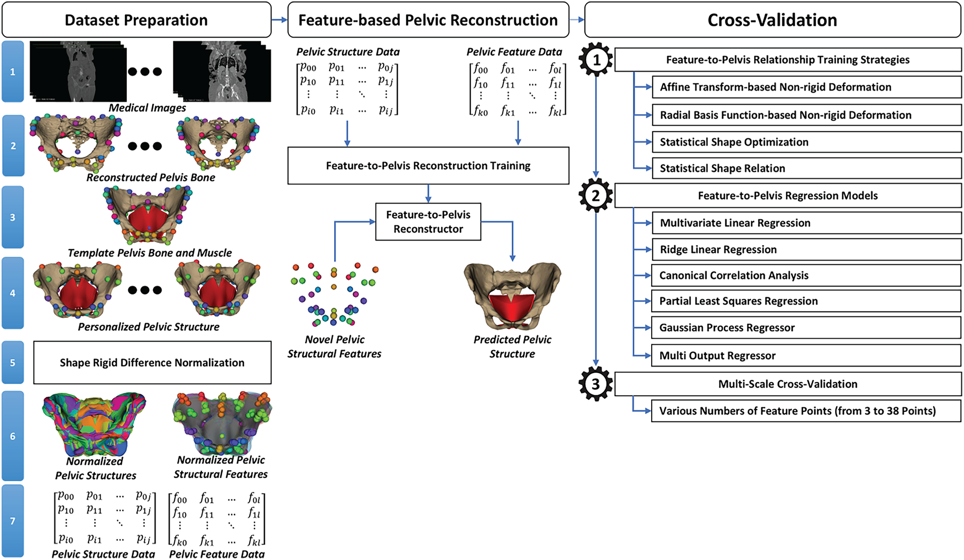
Figure 1: The overall processing procedure of the feature-to-shape pelvic structure reconstruction.

During data set preparation, medical images, such as Computed Tomography (CT) scans of the torso region from healthy subjects, were first collected from publicly available databases. Pelvic bone structures were then manually reconstructed from the selected medical image sets. For each reconstructed pelvis surface mesh, we also defined and selected anatomical landmarks to support dataset alignment. A template pelvic structure including bones and muscles was designed based on the anatomical structure of the human pelvic bone and muscle using Computer-Aided Design (CAD) software, e.g., SolidWorks [26]. A cascading non-rigid deformation was employed to personalize the template pelvic structure to the CT-reconstructed pelvic bone mesh. This cascading procedure included (a) rigid registration for transforming the template mesh to the coordinate system of the CT-reconstructed pelvic bone mesh based on the anatomical landmarks defined on both the template and CT-reconstructed pelvic bone meshes, (b) affine and non-rigid deformation processes for refining alignment and propagating displacements to pelvic muscles and joints, and (c) region-of-Interest (ROI) fine deformation for ensuring local anatomical fidelity. We also defined structural feature points on the personalized pelvic bones for studying their relationship with the pelvic structure. Note that the anatomical landmarks are different from the structural features. The anatomical landmarks were manually selected on the CT-based pelvic bone meshes supporting the pelvic structure personalization. The structural features were defined on template pelvic bone meshes for studying the relationships between pelvic features and structures.

Based on the anatomical landmarks, the personalized pelvic structures and features were then rigidly transformed to the first pelvic structure before normalizing to the origin of the global coordinate system. Finally, the pelvic structure and pelvic feature data were derived from the personalized geometries. The details of dataset preparation will be presented in Section 2.2.

In the feature-based pelvic reconstruction, we trained the relationship between pelvic feature data and pelvic structure data, known as the feature-to-pelvis relationship. Based on the trained relationship, a novel pelvic structure could be reconstructed from novel pelvic structural features. Note that the feature data were the numeric matrix formed by the coordinate values of the 3-D structural feature points of all the personalized pelvic bone and muscle meshes. The pelvic structure data were formed by the coordinate values of all the vertices of the personalized pelvic bone and muscle meshes. The feature-to-pelvis relationship was trained through their shape parameters using multivariate regression. The shape parameters of the pelvic features were computed from the PCA (principal component analysis)-based shape model trained from the pelvic feature data. The shape parameters of the pelvic structure were also computed from the PCA-based shape model trained from the pelvic structure data. With the trained PCA-based shape models of the pelvic structure and pelvic features coupled with a regression model, the pelvic structure can be predicted from a new set of pelvic structural features. The details of feature-based pelvic reconstruction will be presented in Section 2.3.

In the cross-validation, the feature-to-pelvis reconstruction was validated with various reconstruction strategies, including affine transformation-based non-rigid deformation [27], radial basis function (RBF)-based non-rigid deformation [28], statistical shape optimization [29], and statistical shape relation [30], to select the optimal reconstruction strategy. In the affine transformation-based reconstruction strategy, an affine transformation was estimated from the template to target pelvic structural features. The estimated affine transform was applied to the vertices of the template pelvic structure to form the generated pelvic structure. In the radial basis function-based reconstruction strategy, the deformation information from the template pelvic features to the target pelvic features was propagated to the vertices of the template pelvic structures to form the generated pelvic structures. In the statistical shape optimization-based reconstruction strategy, the shape parameters of the PCA-based shape model trained from pelvic structure data were optimized so that the structural features of the PCA-based shape model were optimally fitted with the target pelvic features. In the statistical shape relation-based reconstruction strategy, the pelvic structure was predicted straightforwardly from the pelvic structural features. The prediction was conducted by the trained multivariate regression model from the PCA shape parameters of the pelvic features to the PCA shape parameters of the pelvic structures. Various multivariate regression models were tried, including linear regression [31], ridge linear regression [32], canonical correlation analysis [33], partial least squares regression [34], Gaussian process regressor [35], and multioutput regression [36]. We also validated the relationship between the method’s accuracy and the number of structural features. The whole dataset was split into fitting, validation, and testing sets using 10-fold cross-validation. The details of the cross-validation will be presented in Section 2.4.

2.2 Dataset Preparation

2.2.1 Pelvis Bone Reconstruction from Medical Images

Fig. 2 illustrates the detailed process of reconstructing the pelvic bone structure from medical images. We collected medical images from two public datasets: the New Mexico Decedent Imaging Database (NMDID) [37] and the CTPelvic1K [38]. In the NMDID, the collected medical images were mostly Computed Tomography (CT) images. This database includes more than 15,000 decedents imaged between mid-2010 and mid-2017, comprising approximately 4000 CT slices, with an image size (width × height) of 512 × 12 per individual. These slices were acquired optimally for specific regions of the body, with the slice thickness ranging from 0.5 to 1 mm. In this study, we acquired 100 CT image sets of the torso region from female subjects. The selected subjects must have the ages over 18 years old and have normal pelvic structures. A Data Use Agreement (DUA) form was completed for research-oriented data usage. The second database is the CTPelvic1K dataset [38], including over 320,000 axial slices with approximately 1184 3-D volumes of the pelvic region from adult subjects. Note that the CTPelvic1K was formed by seven sub-datasets: ABDOMEN [39], COLONOG [38], MSD_T10 [40], KITS19 [41], CERVIX [38], CLINIC [42], and CLINIC-metal [38]. The slice thickness of this dataset ranges from 0.8 to 3.8 mm. In this study, we selected only 1106 adult subjects with normal and fully visible pelvic structures inside the 3-D CT volumes. The CTPelvic1K was distributed to the public with the license of Commons Attribution–NonCommercial–ShareAlike 4.0 International (CC BY-NC-SA 4.0) [43] to be used for non-commercial purposes only.

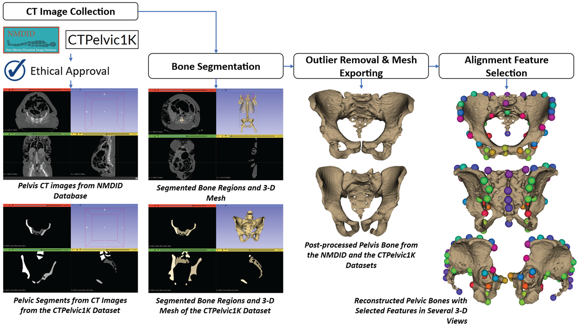
Figure 2: Illustration of the reconstructing process of the pelvis bone from CT images.

After collecting the medical images, the pelvic bone pixels must be segmented from each slice. Regarding the CT images collected from the NMDID dataset, each CT image set was imported into the 3-D Slicer software [44] for segmentation. The pixel intensity level was manually selected so that the segmented regions covered most pelvic bone structures on each slice. The segmented regions of all slices of the CT image set were then converted into a 3-D surface mesh using the marching cube algorithm [45]. The reconstructed bone meshes might contain outliers and non-pelvic bones, so they were removed from the reconstructed bone meshes using the mesh cutting tool inside the 3-D Slicer [44]. Specifically, the femoral heads were separated from the pelvic structures by manually erasing their corresponding voxels slice by slice. Regarding the CT images collected from the CTPelvic1K [38] dataset, this dataset includes pre-segmented pelvic bone structures, so we just input the segments into the 3-D Slicer software [44] and convert these segmentations into pelvic bone meshes using the marching cube algorithm [45]. The reconstructed meshes were post-processed to keep only the pelvic bone structures. All post-processed pelvic bone meshes were exported into mesh files with the Stanford Triangle Format (*.ply) [46]. Note that, for the CTPelvic1K [38] dataset, after reconstruction, we classified the gender of the reconstructed pelvic meshes and selected about 200 female subjects. The classification criteria are the differences in geometrical structures between the male and female subjects [47,48].

Finally, for each pelvic bone mesh, we defined anatomical landmarks supporting dataset alignment. The landmark positions were defined based on the pelvic anatomical structures [49–53]. In addition to the standard landmarks, we also refined landmark selection to optimize data alignment, as presented in Section 2.2.4. The landmark selection was conducted using MeshLab software by our senior students in the biomedical engineering program, who were well-trained in human anatomy. Fifty-three anatomical landmarks were picked for all pelvic bone structures in the dataset.

2.2.2 Template Pelvic Bone and Muscle Designs

Based on the pelvic anatomical structure [54–56], we defined a template biomechanical pelvic structure. In this study, the muscles were not segmented from medical images. Instead, they were manually designed using a Computer-Aided Design (CAD) workflow guided by anatomical references and knowledge. The template pelvic structure includes a high-resolution pelvic bone model extracted from a publicly available MRI dataset, combined with CAD-designed pelvic floor and perineal muscles validated by anatomical experts. As shown in Fig. 3, the pelvic structure includes both pelvic bones and muscles. The pelvic bones consist of the left ilium, the right ilium, the sacrum, the left sacroiliac joint, the right sacroiliac joint, and the pubic joint. The pelvic muscles include the pelvic floor muscle, the superficial transverse perineal muscle, the external anal sphincter muscle, the ischiocavernosus muscle, and the deep transverse perineal muscle.

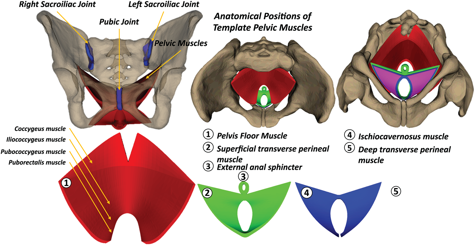
Figure 3: Pelvic floor and perineal muscle shapes designed using a Computer-Aided Design (CAD) approach.

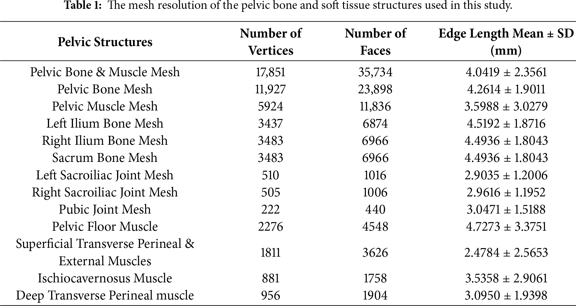
The pelvic bone structure was extracted from the bony pelvis model reconstructed from a high-resolution MRI dataset of a 25-year-old cis-female subject, developed by the Oklahoma State University Biomedical Imaging Laboratory. This model was distributed to the public on the https://sketchfab.com website with the Creative Commons Attribution (CC BY) license. Because the extracted pelvic structure did not include the pelvic muscles, we designed all main types of pelvic muscles with the CAD software, e.g., SolidWorks [26]. The pelvic bone and muscle structures have been checked to ensure suitability for later biomechanical simulation using the Finite Element Method (FEM). The mesh resolution information of the pelvic bone and muscle structures is listed in Table 1. In particular, the numbers of vertices for the pelvic bone & muscle mesh, pelvic bone mesh, and pelvic muscle mesh are 17,851, 11,927, and 5924, respectively. The average edge lengths of the pelvic structure range from 2.478 to 4.494 mm. These mesh resolutions are acceptable and good for FEM simulation [57]. The designed template pelvic structure would be used for dataset alignment throughout all subjects in the dataset.

2.2.3 Pelvic Structural Feature Point Definition

In addition to the anatomical landmarks supporting data alignment, we also defined the structural features of the template pelvic structure. The positions of the structural features are the same as those of the anatomical landmarks, but the number of points is smaller than that of the anatomical landmarks. This is because the structural pelvic features will be manually selected by the user in the axial view of the medical image slice to reconstruct the entire pelvic structure. Consequently, these structural features must be simplified and not include full details, as in the case of anatomical landmarks. The numbers and positions of the pelvic structural features are shown in Fig. 4. The number of structural features ranges from 3 to 38 points. The positions of structural features were selected based on the anatomical structures of the pelvis [58–61]. In the feature-to-structure prediction procedure, the morphometry of pelvic structural features is pre-selected by the user based on the requirement for pelvic reconstruction accuracy. The relationship between the morphometry of the pelvic structural features and the pelvic reconstruction accuracy will be presented in Section 3.3.

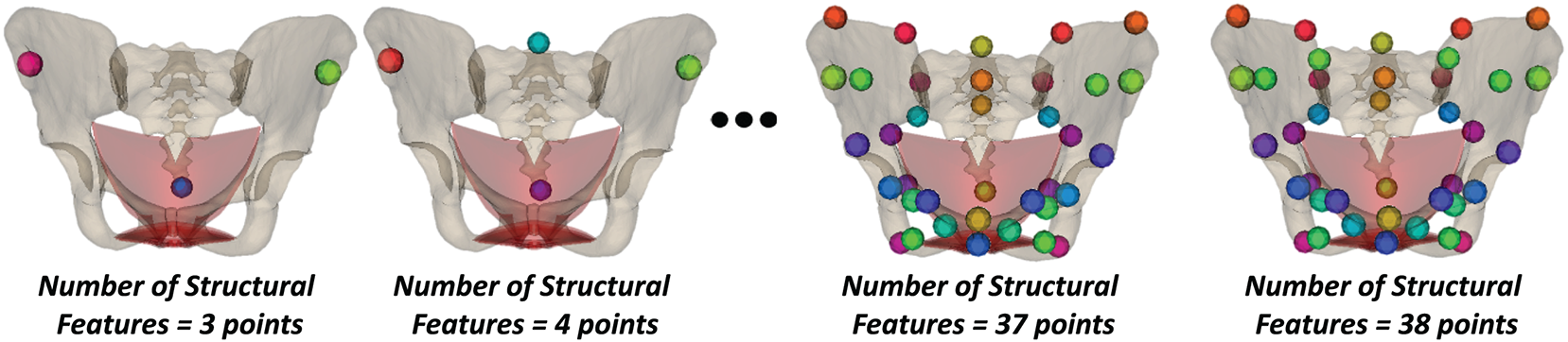
Figure 4: The definition of the feature points for predicting the pelvic structures.

It is important to note that the structural features were selected on the template pelvic bone-muscle structure only for generating the structural data. However, in practice, the structural features should be manually selected from medical image slices. Fig. 5 illustrates the structural feature points after being manually selected on 2-D image slices and converted into 3-D coordinates using pixel spacing and slice-thickness information.

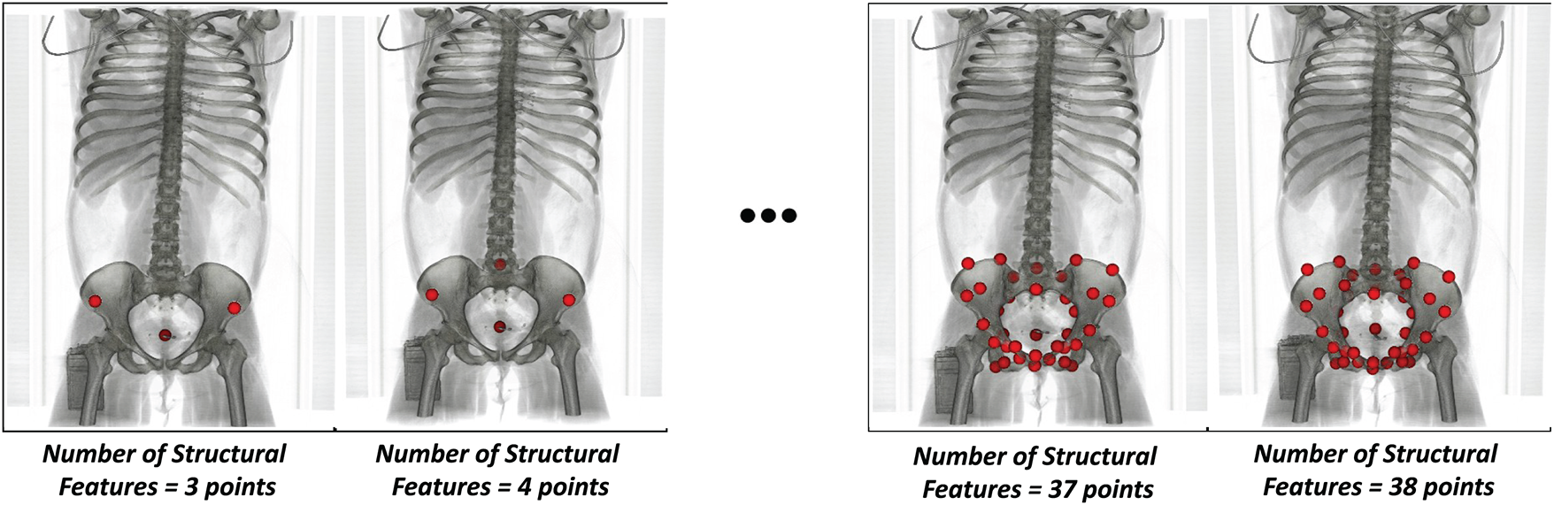
Figure 5: Structural features were manually selected on 2-D image slices and converted to the 3-D space using pixel space and slice thickness values. The features were rendered under the voxel coordinate system. The feature set was set up from 3 to 38 points.

2.2.4 Pelvic Structure Personalization

To align the anatomical and mesh structures of the pelvis across all subjects, we personalized a template pelvic structure for each CT-reconstructed pelvic structure. A cascading coarse-to-fine strategy was developed to deform a template pelvic structure toward the CT-reconstructed pelvic structures. At each stage, different rigid and non-rigid registration methods were applied, with each method contributing to the reduction of rigid and non-rigid shape discrepancies between the template and the CT-based pelvic models.

Specifically, the Singular Value Decomposition (SVD)–based rigid registration [62] initially aligned the template mesh to the coordinate system of the target mesh, thereby removing global rigid differences. The Coherent Point Drift (CPD) affine transformation [63] then provided global scaling to match the size of the source mesh to that of the target mesh. The Non-rigid Iterative Closest Point (Non-rigid ICP) algorithm [64] further deformed the template mesh vertices toward their nearest counterparts on the target mesh while preserving the anatomical plausibility of the pelvic shape through predefined constraints. Importantly, non-rigid ICP must be combined with the preceding SVD and CPD affine registrations to ensure consistent pelvic orientation, size, and anatomical positioning before addressing the remaining morphological shape variation between the meshes. Finally, the Radial Basis Function with a Thin-Plate Spline (TPS) kernel [65] propagated the deformation of the outer bounding mesh to its internal structures, functioning similarly to a cage-based deformation approach for personalizing internal anatomy once the external shape is established. Together, these rigid and non-rigid deformation methods effectively transformed the template pelvic structure to match the target anatomy. The complete deformation pipeline is illustrated in Fig. 6, and the pseudocode of the personalization procedure is presented in Appendix A. In particular, this pipeline includes two stages: (1) global shape deformation and (2) Region-of-Interest (ROI) mesh deformation.

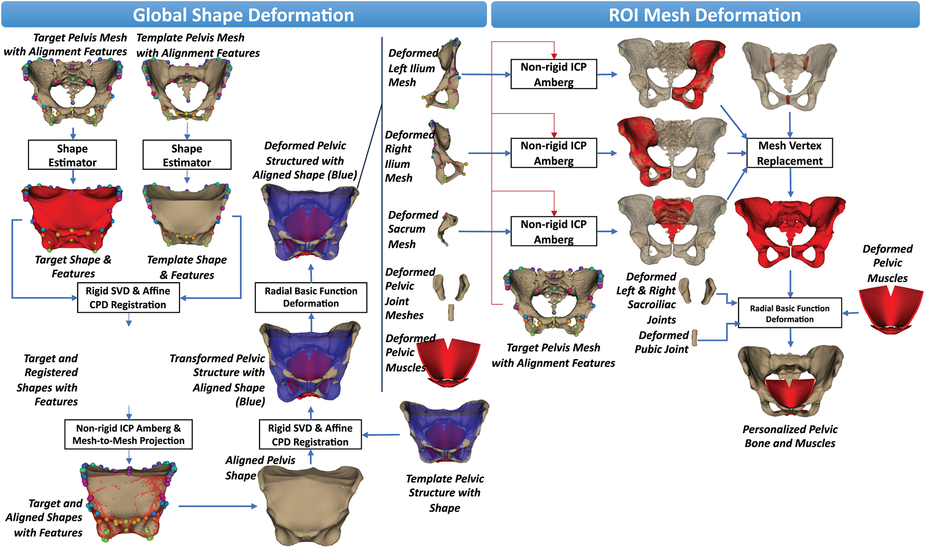
Figure 6: The coarse-to-fine shape personalization process applied to pelvic structures from medical images.

In the global shape deformation, the shapes of the CT-based pelvic bone mesh and the template pelvic bone mesh were first estimated through the shape estimator, as shown in Fig. 6. The template pelvic shape was then registered to the target pelvic shape based on the anatomical landmarks pre-defined on both the target and template pelvic bone meshes. Both rigid deformations using Singular Value Decomposition (SVD) [62] and affine deformations using Coherent Point Drift (CPD) [63] were applied for this registration. The Optimal Step Non-Rigid Iterative Closest Point (Non-Rigid ICP) algorithm [64] was then employed to optimally deform the registered pelvic shape to the target pelvic shape by estimating local affine transformations for each vertex. These local transformations were guided by a stiffness constraint to ensure smooth and anatomically plausible deformation. This algorithm was implemented in the nricp-amberg function of the trimesh library [https://trimesh.org/]. In this function, the stiffness constraint was defined by the default internal settings with a smooth weight of 1 and a global balancing parameter of 1 to ensure smooth and anatomically plausible deformation. Moreover, to ensure the perfect deformation, the vertices of the deformed pelvic shape were projected onto the nearest vertices on the target pelvic shape. Finally, the aligned pelvic shape would have the vertices as the projected vertices and the faces as the faces of the template pelvic shape.

However, the aligned pelvic shape did not include the internal bones and muscles. Consequently, the template pelvic bone-muscle mesh was deformed so that the shape of the template pelvic bone mesh fitted with the aligned pelvic shape. The rigid SVD and non-rigid CPD registrations were used to estimate the SVD-based rigid transform and the CPD-based non-rigid transform to deform the template shape vertices to the target shape vertices. The template pelvic bone-muscle mesh was transformed to the target pelvic shape using the estimated SVD- and CPD-based transformations. As shown in Fig. 6, the transformed pelvic structure is not optimally fitted with the aligned pelvic shape, so we employed the Radial Basis Function (RBF) interpolation with a Thin-plate Spline (TPS) kernel [65] to smoothly propagate vertex displacements across the transformed pelvic bone and muscle meshes. The vertex displacements were computed as the point-to-point displacements from the vertices of the transformed pelvic shape to the vertices of the aligned pelvic shape. The RBF interpolation-based deformation algorithm was implemented using the RBFInterpolator function from the scipy interpolate module [66]. After being interpolated by the vertex displacements, the deformed pelvic bones and muscles had a shape that optimally fit the aligned pelvic shape. However, the pelvic structures inside the shape could not be aligned with those of the target pelvic bones. Consequently, we conducted a fine ROI-based mesh deformation.

In the Region-of-Interest (ROI) mesh deformation, as shown in Fig. 6, the ROI pelvic parts of the deformed pelvic structure include the deformed left ilium, the deformed right ilium, the deformed sacrum, the deformed pelvic joints, and the deformed pelvic muscles. The anatomical landmarks of the appropriate ROI pelvic parts were also computed based on their barycentric coordinates [67] computed concerning the template pelvic structure using the anatomical landmarks defined on the template pelvic mesh. For each ROI pelvic part, we also used the Optimal Step Non-Rigid Iterative Closest Point (Non-Rigid ICP) algorithm [64] to deform the ROI part to the target pelvic mesh. As shown in Fig. 5, each ROI part (rendered in red color) could be optimally fitted with the target pelvic structure. Subsequently, the vertices of the deformed pelvic bone mesh were replaced with the corresponding vertices from each region of interest (ROI), using their predefined vertex indices on the template pelvic bone mesh. The vertex displacements from the vertices of the deformed pelvic bone mesh to the vertices of the personalized pelvic bone mesh were computed. These displacements were smoothly propagated to the vertices of the deformed left sacroiliac joint mesh, the deformed right sacroiliac joint mesh, the pubic joint mesh, and the pelvic muscle mesh to form the appropriate personalized joint and muscle meshes using the Radial Basis Function (RBF) interpolation with a Thin-plate Spline (TPS) kernel [65]. These personalized pelvic parts were concatenated with the personalized pelvic bone mesh to form the personalized pelvic structure.

Regarding pelvic shape estimation from the pelvic bone mesh, as shown in Fig. 7, we first computed the convex hull of the pelvic bone mesh. Note that the convex hull refers to the smallest convex surface that fully encloses the pelvic structure. It provides a simplified outer boundary of the pelvis, which we use to estimate the global pelvic shape before performing detailed concave shape estimation. The estimated convex hull did not have the concave shape of the pelvis, so the convex hull was isotopically re-meshed, called the re-meshed convex hull, before its vertices were projected onto the nearest vertices on the pelvic bone shape. The projected convex hull did not have an isometric facet structure, so it continued to be isometrically re-meshed, called the re-meshed projected convex hull. The vertices of the re-meshed convex hull were then projected onto the nearest vertices of the re-meshed projected convex hull. The procedure of re-meshing the projected convex hull and projecting the vertices of the re-meshed convex hull to the re-meshed projected convex hull was conducted four times. The number of iterations was determined experimentally to ensure the estimated pelvic bone shape did not have sharp corners or edges on its surface. As shown in Fig. 6, the final projected convex hull still has non-isometric facets. Consequently, we finally conducted mesh post-processing to have the final pelvic bone shape. The mesh post-processing included mesh sampling, surface meshing, and mesh hole closing. In the shape estimation, we employed the trimesh library [https://trimesh.org/] for convex hull estimation and the pymeshlab library [https://pymeshlab.readthedocs.io/] for isotropic re-meshing, mesh sampling, and mesh hole closing.

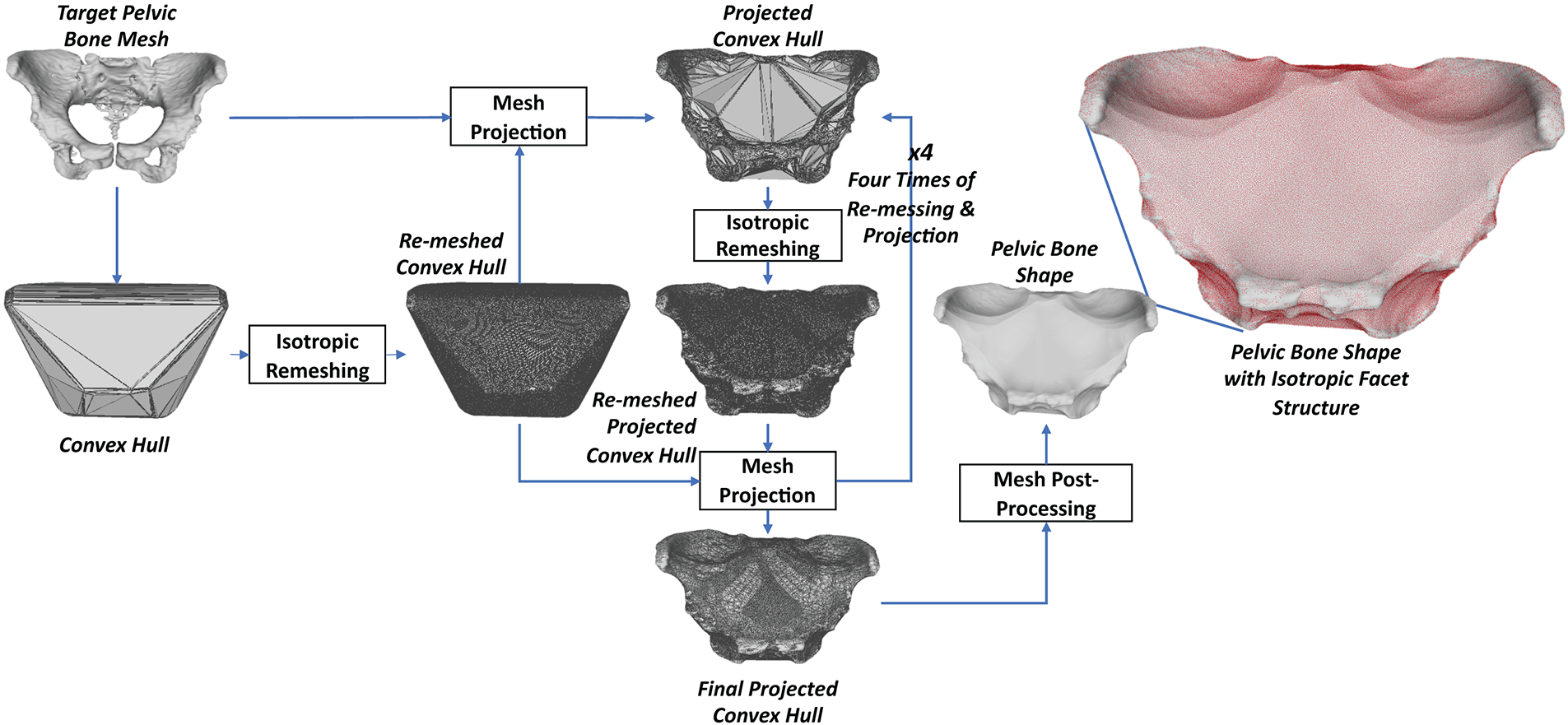
Figure 7: The process for estimating the pelvic bone shape from the pelvic bone mesh.

It is important to note that the personalized pelvic structures of all subjects must be normalized to a standard coordinate system before being analyzed for shape variations. As shown in Fig. 8, normalization begins by rigidly transforming each personalized pelvic structure to the first pelvic structure using the SVD-based registration method. The registered pelvic structures were then transformed to the origin of the global coordinate system. Finally, the coordinate values of the pelvic structural features were formed into the pelvic feature data. The coordinate values of the pelvic structure vertices were formed into the pelvic structure data. The dataset formation will be presented in Section 2.2.5.

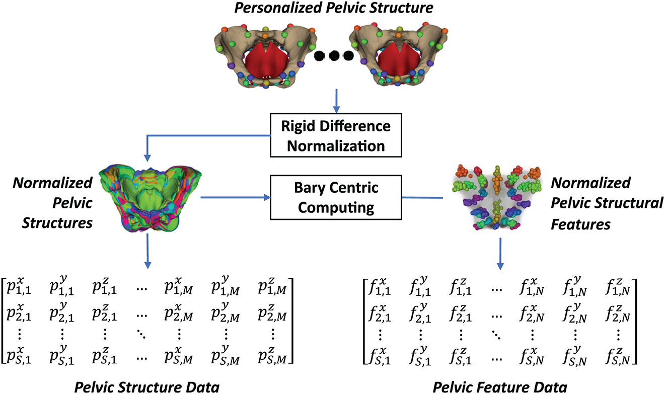
Figure 8: Dataset preparation from the personalized pelvic structures: the personalized pelvic structures were first normalized using the origin of the global coordinate system. The pelvic structural features were computed from the normalized pelvic structures.

2.2.5 Dataset Preparation

The pelvic structural data were formed from the normalized vertices of all personalized pelvic structures. As shown in Eq. (1), the structural data were filled by flattening all vertex coordinates of each pelvic structure into each row of the data matrix.

P=[p1,1xp1,1yp1,1z…p1,Mxp1,Myp1,Mzp2,1xp2,1yp2,1z…p2,Mxp2,Myp2,Mz⋮⋮⋮⋱⋮⋮⋮pS,1xpS,1ypS,1z…pS,MxpS,MypS,Mz]∈RS×3M≡[p11p12…p1Mp21p22…p2M⋮⋮⋱⋮pS1pS2…pSM]∈RS×M(1)

in which,

•   pi,jx, pi,jy, and pi,jz are the x-, y-, and z-coordinate of the vertex j of the pelvic structure i;

•   M=17,851 is the number of vertices of the pelvic structure mesh. Note that, as shown in Fig. 3, the pelvic structure mesh includes the pelvic bone, muscle, and joint meshes.

•   S=300 is the number of subjects in the dataset;

•   P is the pelvic structure data;

•   pij∈R1×3 is the 3-D coordinates of the vertex j in the pelvic structure i.

In addition to the pelvic structure data, pelvic structural feature data were also prepared. As in Eq. (2), the pelvic structural features were computed by their Bary coordinates computed from the template pelvic structure, as shown in Fig. 4.

fj=λaPa+λbPb+λcPc;λa+λb+λc=1;λa,λb,λc≥0(2)

in which,

•   fj∈R3 is the structural feature j.

•   Pa,Pb,Pc∈R3 are 3-D coordinates of the three nearest vertices a,b,c in the template pelvic structure from the feature fj. Note that the k-dimensional tree (KD-Tree) algorithm [68] was employed to determine the nearest vertices.

•   λa,λb,λc are the barycentric coordinates of the feature fj.

The 3-D coordinates of the structural features of the pelvic structure i were also flattened and stored in the line i of the pelvic feature data, as in Eq. (3).

F=[f1,1xf1,1yf1,1z…f1,Nxf1,Nyf1,Nzf2,1xf2,1yf2,1z…f2,Nxf2,Nyf2,Nz⋮⋮⋮⋱⋮⋮⋮fS,1xfS,1yfS,1z…fS,NxfS,NyfS,Nz]∈RS×3N≡[f11f12…f1Nf21f22…f2N⋮⋮⋱⋮fS1fS2…fSN]∈RS×N(3)

in which,

•   fi,jx, fi,jy, and fi,jz are the x-, y-, and z-coordinate of the feature j of the pelvic structure i,

•   N=3,4,5,…,38 is the number of structural feature points, as shown in Fig. 4,

•   F is the pelvic feature data,

•   fij∈R1×3 is the 3-D coordinates of the structural feature j of the pelvic structure i.

2.3 Feature-Based Pelvic Reconstruction Strategies

2.3.1 Affine Transform-Based Non-Rigid Deformation

Appendix B presents the pseudocode of using an affine transform to reconstruct the pelvic structure from the pelvic structural features, and Fig. 9 illustrates the steps of that feature-to-pelvis reconstruction. In particular, the rigid SVD transform was first estimated to transform the template pelvic features to the target pelvic features. The estimated transform was applied to the template pelvic structure to register it to the coordinate system of the target pelvic features. The affine transformation was then estimated to scale the registered pelvic features to the target pelvic features. The estimated affine transform was finally applied to the registered pelvic structure to form the reconstructed pelvic structure.

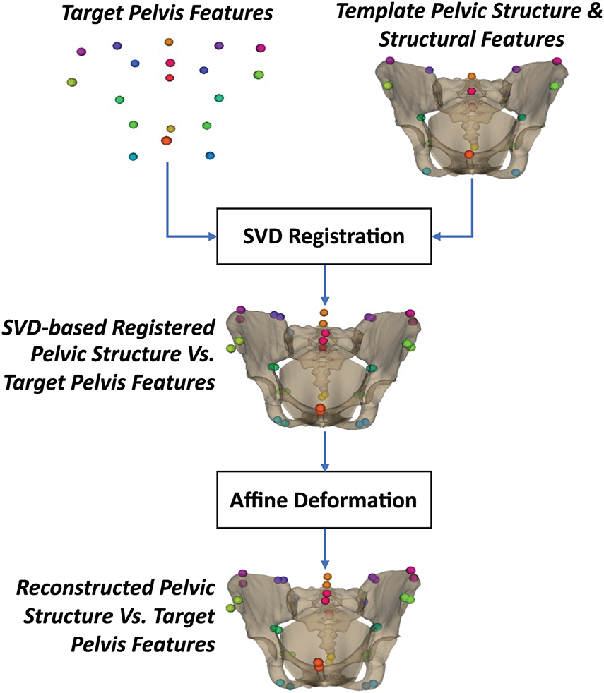
Figure 9: Feature-to-structure reconstruction using affine transform-based non-rigid deformation.

2.3.2 Radial Basis Function-Based Non-Rigid Deformation

Appendix C presents the pseudocode for using radial basis function interpolation to reconstruct the pelvic structure from its structural features. The graphical illustration of each step is shown in Fig. 10. In particular, the template pelvic structure was first optimally deformed to the target pelvic features using the SVD rigid and CPD affine transforms based on the template feature points to form the deformed pelvic structure. The vertex displacements from the deformed pelvic features to the target pelvic features were computed. These vertex displacements were then propagated to the vertices of the deformed pelvic structure using the RBF interpolation with the TPS kernel [65] to yield the reconstructed pelvic structure. Note that although the RBF (TPS) interpolation is capable of non-rigid deformation, it is applied only after an affine alignment step. The affine transformation removes global differences in position, orientation, and scale between the template and target pelvises, ensuring that the RBF only models local morphological variations. This two-stage approach improves numerical stability and prevents the RBF from producing unrealistic global distortions.

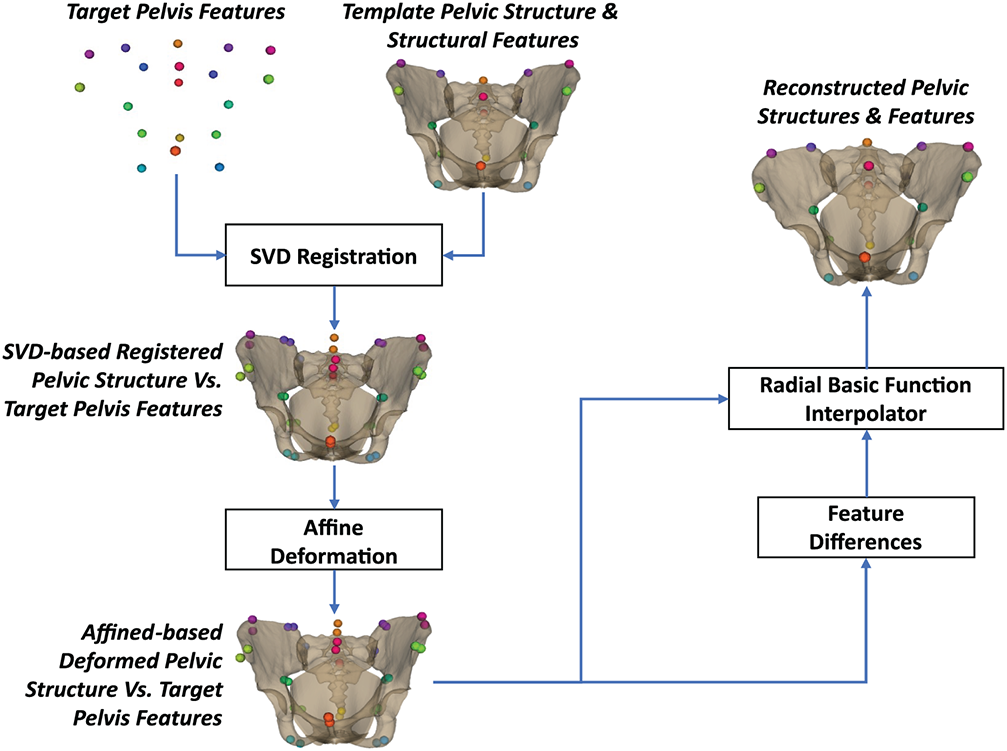
Figure 10: Feature-to-structure reconstruction using radial basis function-based non-rigid deformation.

2.3.3 Statistical Shape Optimization

Appendix D presents the pseudocode of using a statistical shape optimization strategy for reconstructing the pelvic structure from the pelvic structural feature points, and the illustration of each step is shown in Fig. 11. In particular, we fitted the statistical shape model of the pelvic structure to the fitting structural data Ptrain, as in Fig. 1. The principal component analysis (PCA) [69] was employed for statistical shape modeling. The shape of any new or reconstructed pelvic structure S∈R3M can be approximated as in Eq. (4).

S=S¯+Bw(4)

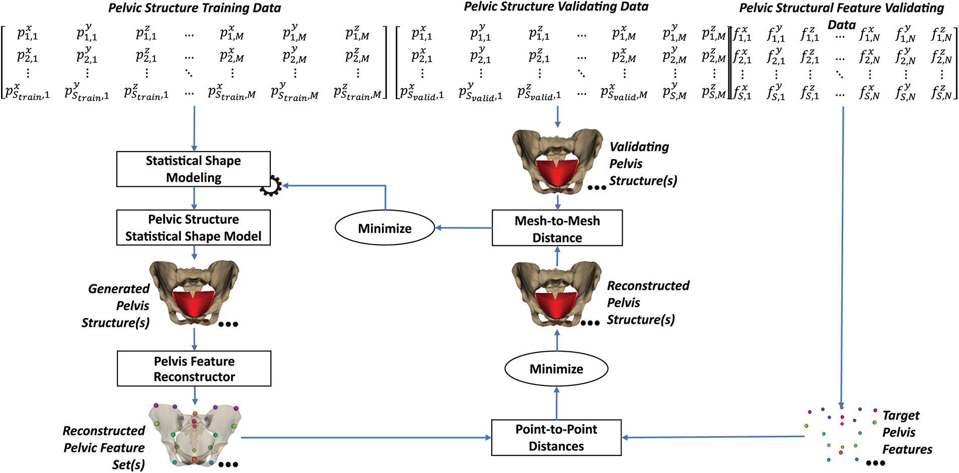
Figure 11: Feature-to-structure reconstruction using statistical shape optimization.

In which,

•   S¯∈R3M is the mean shape vector of the pelvic structure,

•   B∈R3M×K contains the first K principal components (eigenvectors),

•   w∈RK is the vector of shape parameters (weights) that control the deformation of the mean.

The parameters of the pelvic SSM, w was optimized to control the shape of the pelvic structure S so that its features fit with the target features. The reconstructed pelvic structures were compared with the validating pelvic structures to determine the optimal number of components for the SSM. A ten-fold cross-validation procedure was conducted for selecting the optimal component numbers. The least squares algorithm was employed for SSM optimization.

2.3.4 Shape Relation-Based Prediction

Fig. 12 illustrates the process of reconstructing pelvic structure from the pelvic structure based on the feature-to-structure relationship. The pseudocode of this prediction procedure is presented in Appendix E. In the fitting data, the pelvic structure and its features were parameterized into the structure SSM and the feature SSM using the PCA, as shown in Eqs. (5) and (6).

p=p¯+Bpρ(5)

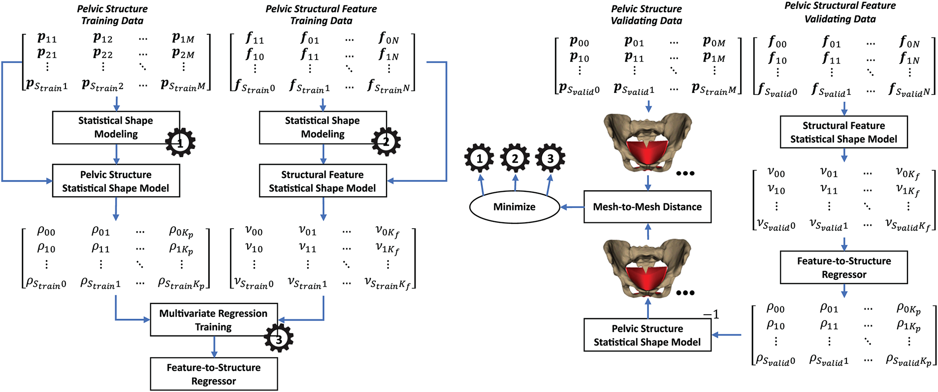
Figure 12: Feature-to-structure reconstruction using shape relation-based prediction.

f=f¯+Bfν(6)

in which,

•   p∈R1×3M is the vectorized 3-D shape of a pelvic structure,

•   p¯∈R1×3M is the mean vectorized 3-D shape of the pelvic structures,

•   Bp∈R3M×Kp is the matrix of principal components of pelvic structures,

•   ρ∈RKp is the shape parameter for controlling the pelvic structure variation,

•   Kp is the number of components of the pelvic structure SSM,

•   f∈R1×3N is the vectorized 3-D shape of a pelvic feature set,

•   f¯∈R1×3N is the mean vectorized 3-D shape of the pelvic feature sets,

•   Bf∈R3N×Kf is the matrix of principal components of the pelvic feature sets,

•   ν∈RKf is the shape parameter for controlling the pelvic feature variation,

•   Kf is the number of components of the pelvic feature SSM.

Based on the fitted structure SSM and feature SSM, the structure and feature fitting data were transformed into the corresponding parameter sets. The feature-to-structure relationship was trained through the relationship between the feature parameters and the structure parameters using multivariate regression.

In the validation stage, the trained feature SSM was used to transform the pelvic structural feature validation data into the pelvic structural validation parameter sets. The validating feature parameter sets were used to predict the structure parameter sets using the trained feature-to-structure multivariate regression. The predicted structure parameter sets were finally inverse-transformed to the predicted pelvic structure using the trained pelvic structure SSM. The predicted pelvic structures were compared with the validating pelvic structures for hyper-parameter tuning. The hyperparameters included the number of components of the feature and structure SSMs and the types of feature-to-structure multivariate models.

2.4 Cross-Validation

To evaluate the quality of the pelvic structure personalization, we computed the mean mesh-to-mesh distances between the personalized pelvic bone meshes and the CT-reconstructed pelvic bone meshes. The mean mesh-to-mesh distances were computed using Eqs. (1) and (2). Moreover, to illustrate the variability of the pelvic structure statistical shape model (SSM), we employed the Principal Component Analysis algorithm to parameterize the shape variability of the personalized pelvic bone and muscle meshes. The explained variance plot, cumulative explained variance plot, and variation visualization were drawn to evaluate the quality of the pelvic SSM. Note that before fitting the PCA-based shape model, the fitting data were normalized using the standard normalizer [70]. The fitting data were formed so that each row contains all flattened vertices of each personalized pelvic structure.

A multi-level ten-fold cross-validation procedure to tune the hyperparameters of the feature-to-structure reconstruction procedure. The hyperparameters in this procedure included the feature-to-structure reconstruction strategies, the types of feature-to-structure multivariate regressors, and the number of pelvic structure features. The whole dataset was divided into two sub-datasets: the cross-validation set and the evaluation set. In this study, we selected 100 female subjects from the NMDID database [37] as the cross-validation set and 200 adult female subjects collected from the CTPelvic1K database [38] as the evaluation set. The cross-validation set was split into a fitting set (80%) and a validation set (20%).

To select the optimal reconstruction strategy, four feature-to-structure reconstruction strategies were evaluated: affine transform-based non-rigid deformation, radial basis function-based non-rigid deformation, statistical shape optimization, and statistical shape relation. At this stage, the cross-validation set was employed. It is important to note that, during this cross-validation stage, the number of structural feature points was fixed at 16. The optimal reconstruction strategy was identified as the one that yielded the lowest validation error after optimization. The fitting and validating processes were conducted on the cross-validation set.

Regarding the affine transform-based non-rigid deformation strategy, as presented in Section 2.3.1, because we did not need to tune the hyperparameters, the strategy was used directly to predict pelvic structures from structural features and was compared with the ground-truth pelvic structures in the validation set. The mean mesh-to-mesh distances were used for these comparisons.

Regarding the Radial Basis Function-based non-rigid deformation strategy, as presented in Section 2.3.2, we also predict the pelvic structures from the structural features and compared them with the ground truth pelvic structures in the validation set. The mean mesh-to-mesh distances were also used for this comparison.

Regarding the statistical shape optimization strategy, as presented in Section 2.3.3, the SSM of the pelvic structure was trained on the pelvic structure validation data. The parameters of the trained SSM were optimized so that the reconstructed structural features were fitted with the structural features in the validation set. The optimized pelvic structures were finally compared with the ground truth pelvic structures in the validation set. For each ten-fold cross-validation, the number of components of the pelvic structure SSM was increased from 1 to 80, as we only had 80 subjects in the fitting set. The optimal number of components corresponded to the minimum validation error. The mean mesh-to-mesh distances were used for this comparison.

Regarding the statistical shape relation strategy, as presented in Section 2.3.4, the pelvic structures and pelvic features in the fitting set were parameterized into the pelvic structure and pelvic feature parameter sets. The relationship between the feature parameters and the structure features was trained using multivariate regression. In this case, the multivariate linear regression model was employed. In the validation process, structural features in the validation set were parameterized using the trained feature SSM. The pelvic structure parameters were predicted from the feature parameters using the trained multivariate linear regression. The predicted structure parameters were used to reconstruct the pelvic structures using the trained structure SSM. The reconstructed pelvic structures were compared with the ground truth pelvic structures in the validation set using the mesh-to-mesh distance metric. For each ten-fold cross-validation, the number of components of the feature SSM and the structure SSM was increased from 1 to 80, as we only had 80 subjects in the fitting set. It is important to note that, since the number of structural feature points was fixed at 16, the maximum number of components for the feature SSM was limited to 48. The optimal number of components was selected as the one that minimized the validation errors.

To select the optimal multivariate regression model, the statistical shape relation strategy was trained and validated using various regression techniques, including linear regression, ridge linear regression, canonical correlation analysis (CCA), partial least squares regression (PLSR), Gaussian process regression (GPR), and multioutput regression. At this stage, the cross-validation set was employed. For each model type, the optimal number of components for both the feature and the structure SSMs was identified through validation error minimization. The optimal regression model was determined as the one that achieved the lowest average validation error across the cross-validation folds.

To select the optimal number of structural features, the optimal feature-to-structure reconstruction strategy coupled with the best multivariate regression model (if the optimal strategy was the statistical shape relation) was trained with the number of structural features increasing from 3 to 38. For each number of structural features, the optimal number of PCA components was determined as which had the minimum mean error on the validation sets throughout a ten-fold cross-validation. The optimal number of feature points was identified as having the minimum mean error on the testing sets throughout a ten-fold cross-validation. Note that at this stage, the full dataset (including the 100 female subjects from the NMDID and the 200 female subjects from the CTPelvic1K databases) with its fitting set (70%), validating set (20%), and testing set (10%) was employed. The testing errors were computed between the predicted and reference pelvic structures. The reference pelvic structures could be the personalized pelvic bone meshes, the personalized pelvic bone and muscle meshes, and the CT-based pelvic bone meshes. Last but not least, to evaluate the accuracy of the predicted pelvic muscle, we also computed the testing errors between the predicted pelvic bone meshes and the CT-based pelvic bone meshes on the muscle attachment point regions. To determine the muscle attachment regions, we manually pick feature points of the muscle attachment points on the template pelvic bone mesh. The regions were defined as spheres having the centers as the picked feature points and a radius of 6 mm.

To illustrate the distribution of the prediction error in various regions of the pelvic bone mesh, we also computed the vertex-to-surface distances between the predicted pelvic structure’s vertices and the reference pelvic structures. The distance from the ith vertex pi from a predicted pelvic bone mesh to the reference surface mesh, R, is computed using Eq. (7). The reference pelvic structure could be the personalized pelvic bone meshes, the personalized pelvic bone muscle meshes, or the CT-based pelvic bone mesh. The mean vertex distances were computed on the testing sets throughout the ten-fold cross-validation. The computed mean distance values were illustrated as distance color maps on the template pelvic structure. Note that the optimal feature-to-pelvic structure reconstruction strategy was trained and tested with the optimal number of structural features.

To show the matching between the predicted pelvic bone meshes and the CT-derived ground truth meshes, the best and worst predicted cases on the test sets across ten-fold cross-validation were rendered alongside their corresponding CT-based meshes. Additionally, a representative case was visualized using multi-angle 3-D rendering of a predicted pelvic structure in conjunction with DICOM image slices and the reconstructed 3-D torso shape.

The mesh-to-mesh distance metric was employed to compare the predicted pelvic structure with the reference pelvic structure. This metric is illustrated in Eqs. (7) and (8). In particular, the distance between a vertex of the predicted pelvic structure and the reference pelvic structure was first computed based on the following Eq. (7):

d(pi,R)=min1≤j≤NR‖pi−rj‖2(7)

in which,

•   d(pi,R) is the distance between the ith vertex of the predicted pelvic structure and the reference pelvic structure;

•   P={pi}i=1NP is the predicted mesh vertices. Np is the number of predicted mesh vertices. pi is the ith vertex of the predicted mesh.

•   R={rj}j=1NR is the reference mesh vertices. NR is the number of reference mesh vertices. rj is the jth vertex of the reference mesh.

•   pi,rj∈R3.

The mean value of the mesh-to-mesh distances, computed using Eq. (8), was used to evaluate the difference between the predicted mesh and the reference mesh.

MeanDist(P→R)=1NP∑i=1NPd(pi,R)=1NP∑i=1NPmin1≤j≤NR‖pi−rj‖2(8)

in which,

•   MeanDist(P→R) is the mean distance between the predicted mesh, P, and the reference mesh, R.

It is important to note that although the Hausdorff distance is a commonly used metric for surface comparison, in this study, we employed the mesh-to-mesh distance defined in Eq. (7) and its mean form in Eq. (8). These metrics evaluate, for each vertex on the predicted mesh, the minimum Euclidean distance to the closest vertex on the reference surface. This nearest-neighbor formulation is appropriate for two reasons. First, all predicted meshes are generated by deforming a single template mesh, thereby preserving vertex correspondence and mesh topology across all subjects. As a result, the mesh-to-mesh distance provides an anatomically consistent pointwise error measure when comparing predicted meshes to other predicted meshes. Second, when comparing a predicted mesh to a CT-reconstructed mesh, which does not share the same vertex structure, the nearest-neighbor distance remains suitable because the two surfaces are spatially close after alignment. Under these conditions, the closest-point distance reliably captures local geometric discrepancies between the two surfaces without requiring identical mesh connectivity.

3  Results

3.1 The Pelvic Personzation Accuracy and Shape Variation

Fig. 13 illustrates the error distribution between the personalized and CT-based pelvic structures.

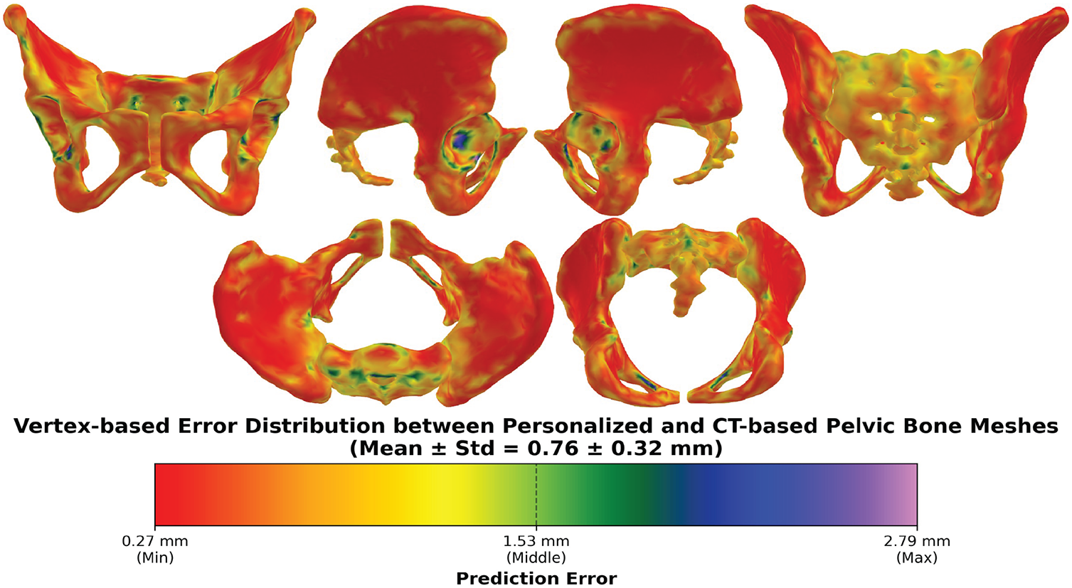
Figure 13: The vertex-based error distribution between the personalized pelvic structures and their corresponding CT-based structures. The mean errors across all subjects were computed and visualized as a color distance map.

The vertex-based mean errors were illustrated as a distance-based color map from red (lowest) to violet (highest) colors. Overall, the grand mean errors and standard deviation were 0.76 ± 0.32 mm. These error values suggest good alignment between the personalized and CT-based pelvic structures. The error range is from the minimum of 0.27 mm to the maximum of 2.79 mm, and most of the pelvic regions are in red to orange colors. This shows that most regions of the pelvic align well with the CT-based pelvic structure, but some small regions deviate more significantly, especially in the sacral promontory & ala, posterior iliac crest, pubic symphysis, ischial spine & tuberosity, anterior inferior iliac spine, and acetabular rim. These regions all have complex curvature, thin ridges, deep concavities, and small variable landmarks, so the personalization process was relatively challenging to fit the template pelvic structure to these complex regions.

Fig. 14 illustrates the explained variance ratio per component of the trained PCA-based statistical shape model of the pelvic structure. In particular, the first principal component alone captures approximately 25% of the total variance in pelvic shape. When the number of components increases, the component’s variance contribution rapidly diminishes. Especially, beyond approximately the 50th principal component, the components contribute negligible variance. The remaining components from 51 to 200 mostly reflect the minor anatomical details. Fig. 15 shows the cumulative variance ratio per component of the pelvic statistical shape model trained from standardized pelvic structures. In particular, the initial components (roughly 50) capture around 95% of the shape variance. After the 50th principal component, the curve nearly flattens. Consequently, the remaining components contribute to the minor details of the pelvic structure.

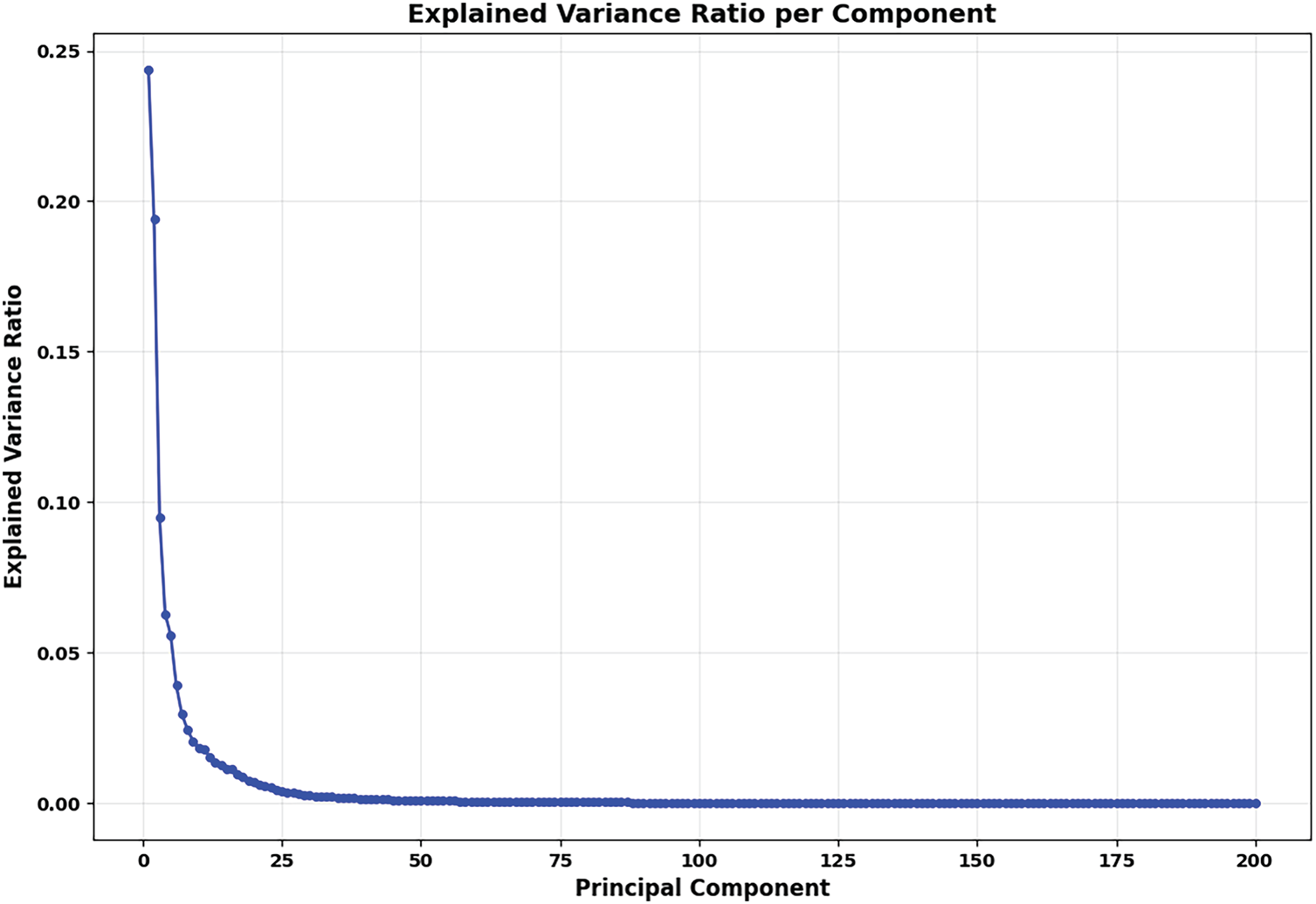
Figure 14: The explained variance ratio per component of the PCA-based shape model of all personalized pelvic structures. The fitting data were standardized before being used for fitting the PCA model.

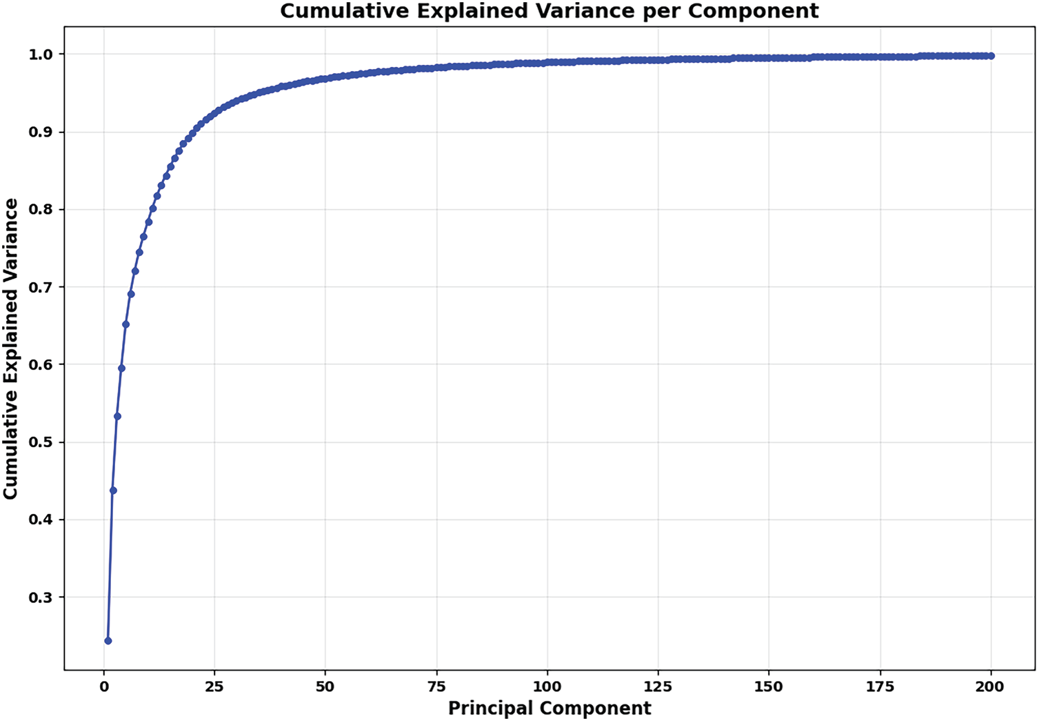
Figure 15: The cumulative explained variance per component of the PCA-based statistical shape model of the personalized pelvic structure. The fitting data were normalized before being used for fitting the PCA model.

Fig. 16 shows the example of shape variance across 10 generated pelvic cases using the trained PCA-based statistical shape model. The overlapping regions are mostly around the iliac wings, sacrum, and pubic arch. This shows that PCA can illustrate morphological differences while preserving structural coherence. Consequently, the shape model of the pelvis can be employed for reconstructing the personalized pelvic structures supporting biomechanical simulations.

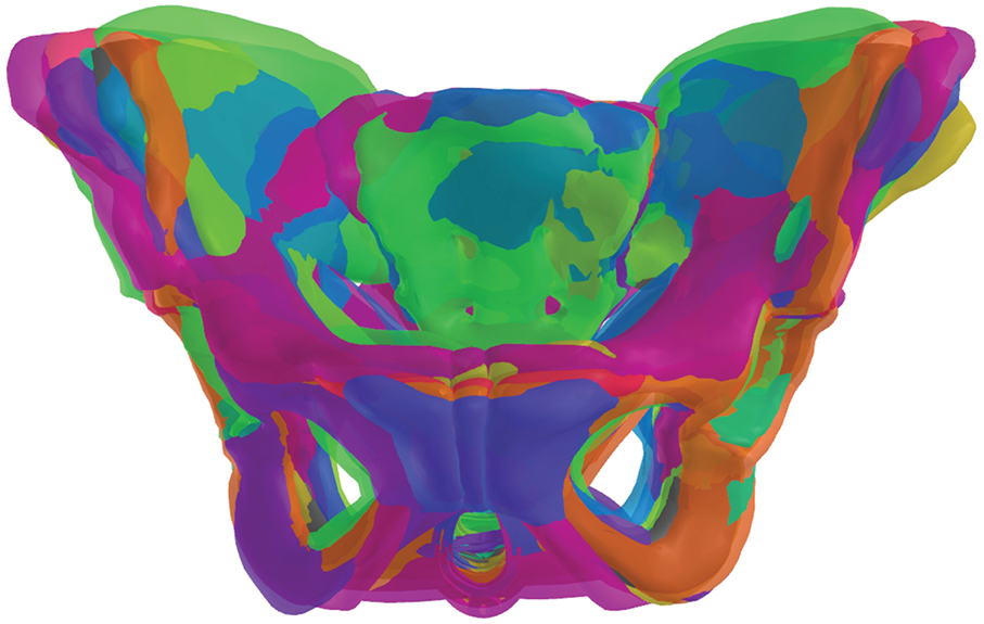
Figure 16: The examples of 10 shape variations rendered on the same coordinate system using the trained PCA-based statistical shape model of the pelvic structures.

Regarding computational efficiency, with the hardware configuration of an HP Zbook 17 G5, Intel(R) Xeon(R) E-2176M CPU @ 2.70 GHz (2.71 GHz) and the installed RAM of 32.0 GB, the time for generating each personalized pelvic structure is 9.5 ± 0.6 min.

3.2 The Optimal Pelvic Reconstruction Strategy

Fig. 17 shows the validation errors between the predicted pelvis bone meshes and the personalized pelvis bone meshes with different feature-to-pelvis reconstruction strategies: affine transform, radial basis function, statistical shape optimization, and statistical shape relation.

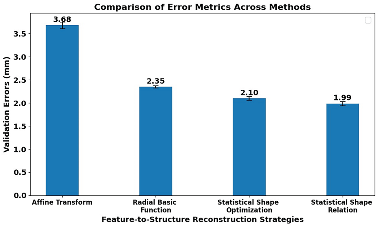
Figure 17: The comparison of validation errors using different strategies for reconstructing pelvic structures from features. The used reconstruction strategies are affine transform-based deformation, radial basis function interpolation-based deformation, statistical shape optimization-based deformation, and statistical shape relation deformation.

In particular, the highest mean validation error is 3.68 mm when using the affine transform-based strategy. This is because the pelvis reconstruction procedure was just based on the affine transform estimated from the structural features of the template pelvis bone mesh to the target pelvis bone mesh, and the pelvis shape variation is complex and cannot be represented by only affine deformation.

With the radial basis function-based strategy, the 3-D movements of the structural features from the template pelvis mesh to the target pelvis mesh were transferred to all vertices of the template pelvis mesh. The degree of freedom of the 3-D feature movements is higher than the affine transformation, so the mean validation error of the radial basis function-based strategy, 2.35 mm, is smaller than that of the affine transform-based strategy, 3.68 mm. However, the number of structural features is much smaller than the number of the pelvis bone mesh’s vertices, so the movements of 3-D structural features are not flexible enough to represent the deformation of the whole pelvic structure. Moreover, the movement of the structural features cannot be fully transferred to the pelvis bone mesh’s vertices due to the constraints of the employed radial basis function.

When using the statistical shape optimization strategy, the deformation of the pelvis bone mesh is more flexible than when using the radial basis function-based strategy because the statistical shape parameters, which were employed for shape optimization, capture the movements of all the vertices on the pelvis mesh. Consequently, the mean validation error of the shape optimization-based strategy is 2.10 mm, which is smaller than that of the radial basis function-based strategy, 2.35 mm.

Other than that, the mean validation error of the statistical shape relation-based strategy can reach 1.99 mm, which is even smaller than that of the statistical shape optimization-based strategy. This is because the shape relation-based strategy trained a statistical mapping between the structural features’ parameters and the pelvis bone mesh’s parameters, which is more robust and generalizable than the shape optimization-based strategy. Moreover, the shape relation-based strategy can reduce overfitting and better capture anatomical variability of both pelvis bone shapes and pelvis structural features, unlike the shape optimization-based strategy, which models only the variability of the pelvis bone shapes.

Based on this analysis and the experimental results, the statistical shape relation-based strategy is the most effective approach for reconstructing pelvic structures from structural features.

3.3 The Optimal Shape Regression Model

Fig. 18 shows mean validation errors between the predicted pelvic bone meshes and the personalized pelvic bone meshes using the statistical shape relation-based feature-to-pelvis reconstruction strategy.

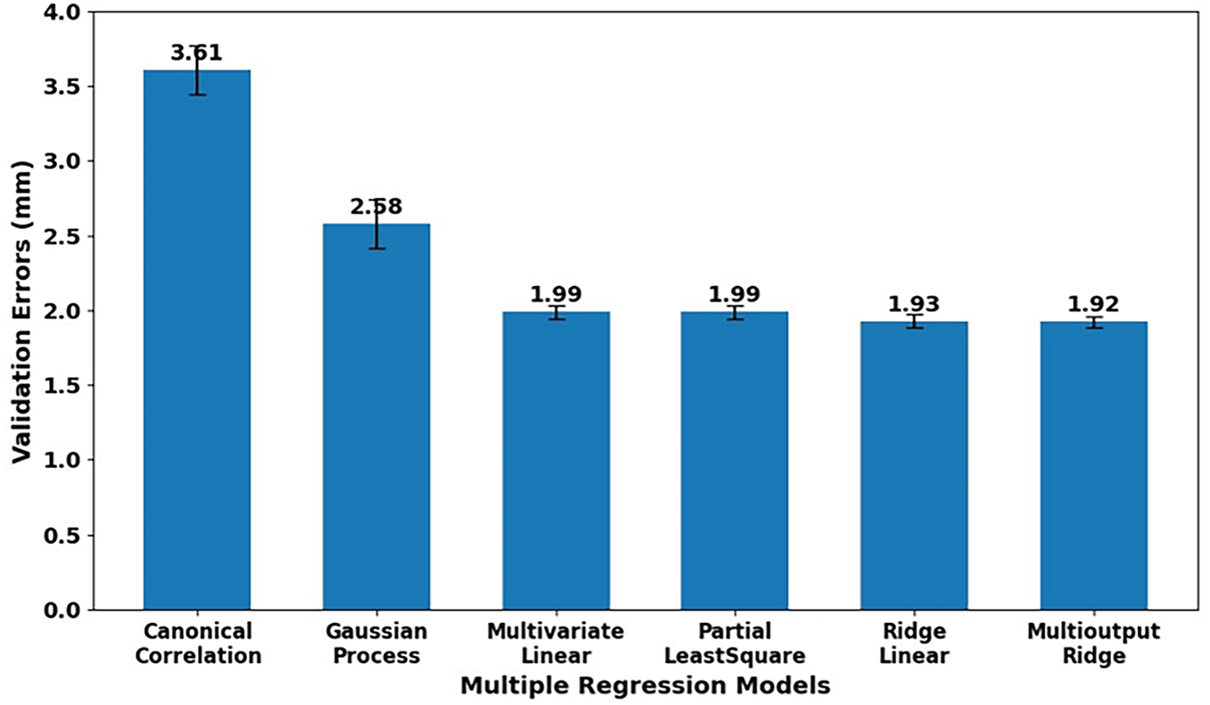
Figure 18: The comparison of validated errors of various regression models when used for predicting pelvic structures from their structural features. The multivariate regression models are canonical correlation-based, Gaussian process-based, multivariate linear, partial least squares, ridge linear, and multioutput with ridge cross-validation.

Various multivariate regression algorithms were employed for estimating the relationship between pelvis bone shape parameters and structural feature parameters. These algorithms included canonical correlation-based regression, Gaussian process-based regression, multivariate linear regression, partial least squares regression, linear regression with ridge, and multioutput ridge regression. Overall, the linear & regularized multivariate regression algorithms outperform the latent variables & kernel-based regression algorithms. The mean validation errors when using the canonical correlation and Gaussian process are 3.61 and 2.58 mm, which are much larger than those when using the linear & regularized regression algorithms, with the mean validation errors around 1.9 mm. This is because the employed principal component analysis (PCA) had transformed the pelvic bone meshes and structural features into a lower-dimensional linear space. Consequently, the relationship between the pelvic feature parameters and the pelvic bone parameters is inherently linear. The latent and kernel-based methods, like Gaussian processes and canonical correlation, assume complex and nonlinear relationships, so they might overfit and misinterpret the simplicity of the relationship between the pelvic feature and pelvic bone PCA-parameters. Based on this analysis, the linear and regularized regression methods are well-suited to capture this linear relationship.

In the linear and regularized regression group, multivariate linear and partial least squares regression (PLSR) have the same mean validation error of 1.99 mm. This is because we selected the target number of components of the PLSR to be the same as the number of parameters of the pelvic bone meshes and the pelvic structural features. Consequently, the PLSR acts in the same way as the multivariate linear regression. It is important to note that the multivariate linear regression and multioutput linear regression coupled with L2 regularization performed better than multivariate linear regressions and partial least squares regressions without L2 regularization. This is because the ridge regression introduced L2 regularization, which penalizes large coefficients. This helps reduce overfitting and stabilizes the solution. In particular, as shown in Fig. 18, the mean validation errors of the two outperforming regression methods are 1.93 and 1.92 mm for the ridge linear regression and ridge multioutput regression, respectively.

In particular, the multioutput ridge regression is even better than the ridge linear regression because it models all the output variables as a unified system, such as the parameters of the pelvic bone mesh, rather than treating each output independently, like the ridge linear regression. This characteristic of multioutput ridge regression helps simulate the interrelation among anatomical regions on the pelvic bone mesh. The L2 regularization contributes to reducing the overfitting and enhancing the generalization when dealing with large numbers of output variables in the multioutput regression method. Consequently, as shown in Fig. 18, the mean validation error of the multioutput ridge regression method is 1.92 mm, which is smaller than the mean validation error of the linear ridge regression method. Based on this analysis, multioutput ridge regression is the optimal multivariate regression method for fitting the relationship between the shape parameters of pelvic structural features and those of pelvic bone meshes.

3.4 Feature-to-Pelvic Structure Prediction Accuracy

Fig. 19 shows the mean errors between the predicted pelvic bone meshes and personalized pelvic bone meshes. The errors were computed on the testing set of the full dataset throughout a ten-fold cross-validation. Note that the statistical shape relation-based feature-to-pelvis reconstruction strategy, coupled with the multiple-output ridge multivariate regression, was employed for cross-validation. In particular, the mean testing errors significantly reduced when the number of structural features increased from 3 to 19 points, with the average decreasing rate of 0.129 mm per point. When the number of structural features increased from 21 to 38 points, the mean testing errors decreased only from 1.863 to 1.664 mm, with an average decreasing rate of 0.012 mm. Ideally, when the number of structural features reaches around 67 points, the mean testing errors can reach zero.

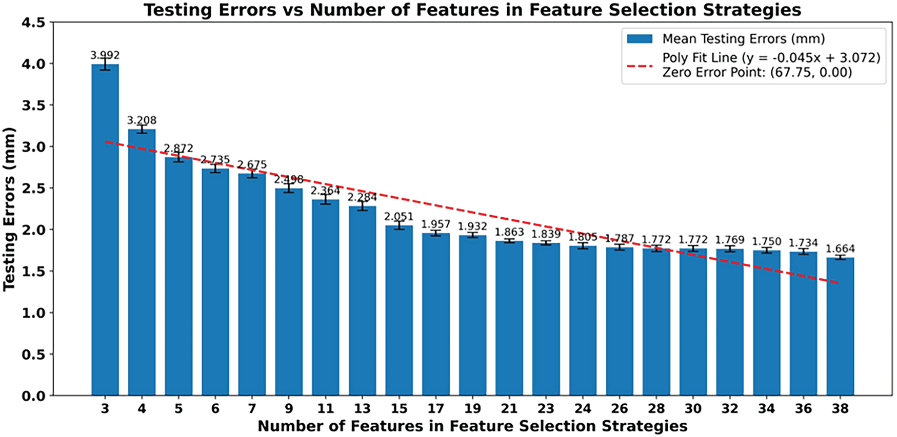
Figure 19: The mean mesh-to-mesh distances between the predicted pelvis bone meshes and the personalized pelvis bone meshes in the testing set of the whole dataset. The testing errors were computed for various numbers of structural features. A linear regression line was also fitted and plotted.

Fig. 20 shows the mean errors between the predicted pelvic bone meshes and the CT-reconstructed pelvic bone meshes across varying numbers of structural features.

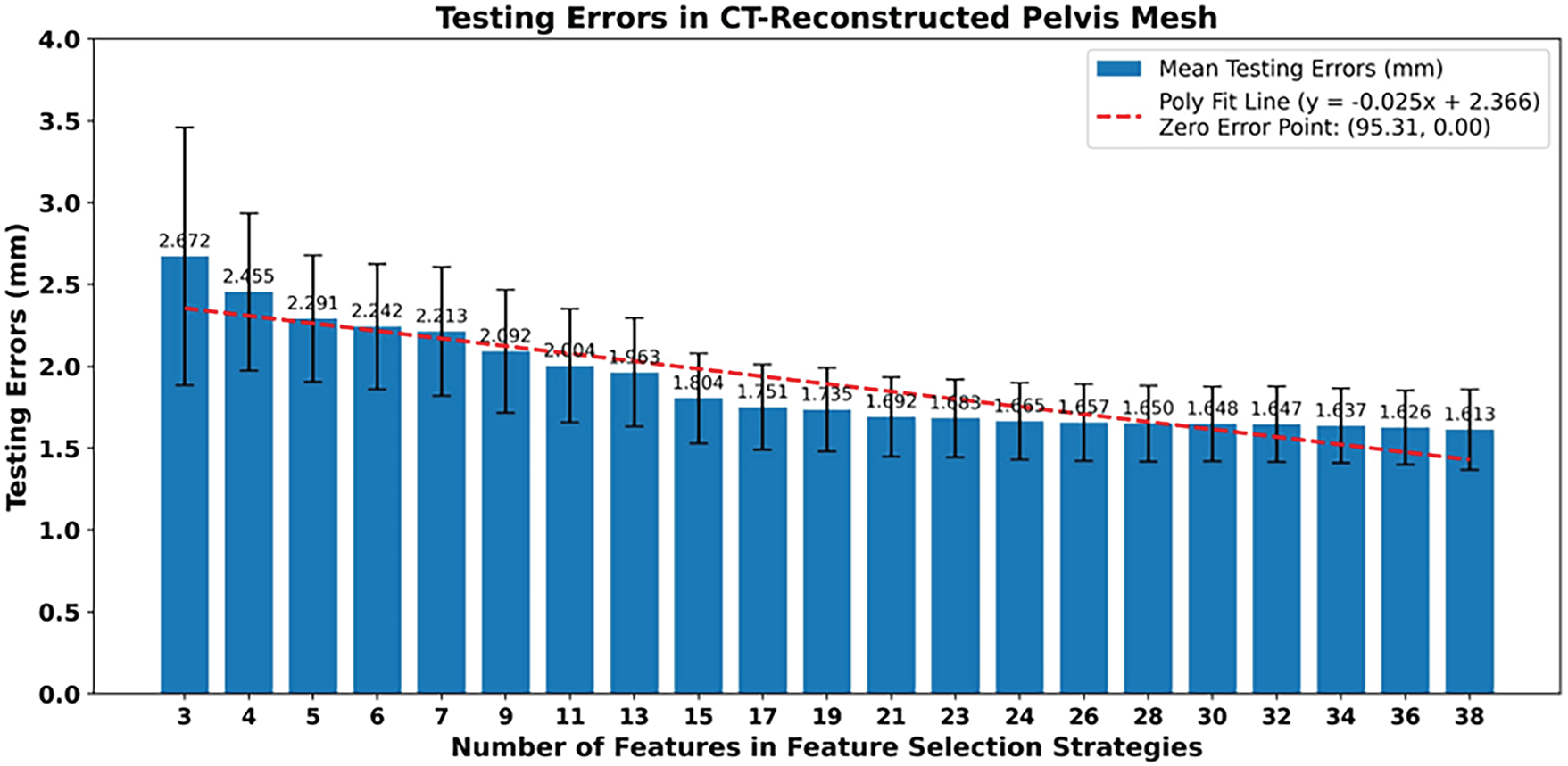
Figure 20: The mean mesh-to-mesh distances between the predicted pelvis bone meshes and the CT-reconstructed pelvis bone meshes in the testing set of the whole dataset. The testing errors were computed for various numbers of structural features. A linear regression line was also fitted and plotted.

The comparison was conducted on the test sets throughout a ten-fold cross-validation on the full dataset using the statistical shape relation-based reconstruction strategy coupled with multioutput ridge regression. In general, the mean testing errors when compared with CT-reconstructed pelvic bone meshes are lower than those when compared with the personalized pelvic bone meshes. In particular, the initial mean testing error is 2.672 mm, which is smaller than 3.992 mm, as shown in Fig. 19. This indicates that the model aligned more closely with CT-based meshes even with the minimal number of structural features. When the numbers of structural features increase from 3 to 19, the mean testing error gradually declines to 1.735 mm, with an average reduction rate of 0.059 mm, which is slower than when comparing with the personalized skull meshes with 0.129 per point. When the number of structural features is from 21 to 38 points, the mean testing errors continue to decrease, from 1.692 to 1.613 mm, with an average reduction rate of 0.005 mm, which is slower than when comparing with the personalized pelvic bone meshes with 0.012 mm per point. Consequently, with more complexity and anatomical precision of the CT-based pelvic bone meshes in comparison with the personalized pelvic bone mesh, the feature-to-pelvic reconstruction model adapts better but slower when increasing the number of structural features. This analysis is also proven by which the polynomial fit line projects a theoretical zero-error point at approximately 95 points, which is higher than when comparing with the personalized pelvic bone meshes with 68 points. This extrapolation implies that denser and more detailed sets of structural features would require to perfect reconstruction of the CT-reconstructed pelvic bone meshes, which are more complex and higher precision anatomical structures than the personalized pelvic bone meshes.

The same correlation behavior between the number of structural features and the mean testing errors was observed in the muscle attachment regions.

Fig. 21 illustrates the mean errors in the muscle attachment regions between the predicted pelvic bone meshes and the CT-reconstructed pelvic bone meshes on the testing sets of the full dataset throughout the ten-fold cross-validation. In this case, a statistical shape relation-based strategy coupled with multioutput ridge regression was employed for fitting and testing. As shown in Fig. 18, the mean testing errors decrease with different reduction rates from 3.237 to 1.415 mm when the number of structural features varies from 3 to 38. Especially, when the number of features is from 3 to 23 points, the mean testing errors in the muscle attachment regions are from 3.237 to 1.731 mm, which are higher than the testing errors in the whole pelvic bone regions, from 2.672 to 1.683 mm. This is because the structural features are not dense enough to illustrate the anatomical positions of muscle attachment points. When the number of features is from 24 to 38 points, the mean testing errors in the muscle attachment regions are from 1.440 to 1.415 mm, which are 13.17% lower than those in the whole pelvic bone structure. This shows that with the number of structural feature points from 24 to 38 points, the feature-to-pelvic reconstruction model can well-predict the anatomical structure of the pelvic bone in the muscle attachment regions with the mean testing errors of 1.427 ± 0.014 mm (Mean ± SD).

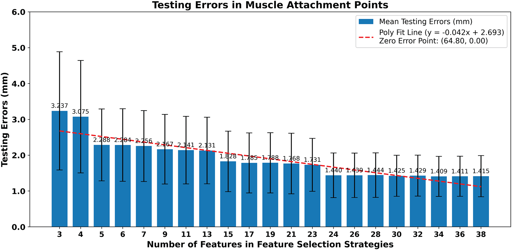
Figure 21: The mean testing mesh-to-mesh distances between the predicted pelvis bone meshes and the CT-reconstructed pelvis bone meshes in the muscle attachment points. The testing errors were computed for various numbers of structural features. A linear regression line was also fitted and plotted.

Based on the analyses of the mean testing errors between the predicted pelvic bone meshes and the personalized pelvic bone meshes, the CT-reconstructed pelvic bone mesh, and the CT-reconstructed muscle attachment regions, as illustrated in Figs. 16–18, respectively, the optimal number of structural features used for pelvic bone mesh reconstruction can be optimally selected from 24 to 38 points. With this number of structural features, the mean testing errors are 1.757 ± 0.043 mm, 1.643 ± 0.017 mm, and 1.427 ± 0.014 mm, when comparing with the personalized pelvic bones, the CT-reconstructed pelvic bones, and the pelvic muscle attachment regions, respectively.

3.5 Regions of Interest Error Distribution

For analyzing the error distribution in various pelvic bones, we also computed point-to-surface distances between the predicted pelvic bone vertices and the target pelvic bone meshes on the testing sets of the full dataset throughout the ten-fold cross-validation. Note that the statistical shape relation-based feature-to-pelvic reconstruction strategy coupled with multioutput ridge regression was employed for fitting and testing. The selected number of structural feature points was 38. The distance values are illustrated as distance color maps.

Figs. 22 and 23 illustrate the error distributions when comparing the personalized pelvic bones with and without pelvic floor muscles, respectively. Overall, without the pelvic floor muscle, the vertex-to-surface distance values range from 0.82 mm to a maximum of 3.51 mm, with a Mean ± SD of 1.77 ± 0.37 mm. The low standard deviation value of 0.37 mm, which is only ~20% of the mean value, illustrates that the errors are relatively consistent across the mesh and have no extreme outliers. The regions with red or orange dominate the central and posterior areas of the pelvis, indicating higher prediction accuracy in these areas. As shown in Fig. 4, higher prediction accuracy is located in the central and posterior areas because more structural feature points were picked in these areas. Regions with blue or green appear around the iliac crest, pubic symphysis, and acetabular rims, suggesting that the anatomical structures in these areas are more challenging to predict from structural features. The higher prediction accuracy in these regions is due to the structural features being less concentrated in these areas than in the others, as shown in Fig. 4. Moreover, the anterior portions of the pelvis tend to have lower errors than the posterior portions of the pelvis because the anterior anatomical structures are less complex than the posterior anatomical structures, especially in the sacrum structures. When the comparison was computed with the pelvic floor muscles, as shown in Fig. 23, the vertex-to-surface distances decreased to 1.59 ± 0.47 mm due to the low distance errors appearing on the pelvic floor region, especially around the levator ani complex, coccygeus, and perineal body. The pelvic floor regions have higher prediction accuracy than the pelvic bones because they have less complex anatomical structures than the bones. It is important to note that some dark green and light blue regions appear at the central pelvic outlet and posterior perineal regions, indicating elevated errors in these regions. This is because of the complex geometry and limited structural features in those regions. The same behavior can be found in the distribution of the vertex-to-surface distances when comparing the predicted pelvic bone mesh with the CT-reconstructed pelvic bones. As shown in Fig. 24, the vertex-to-surface errors are 1.61 ± 0.42 mm and are smaller than when compared with the personalized pelvic structures, which are 1.77 ± 0.37 mm. This is because the CT-reconstructed pelvic bone meshes have higher mesh resolution than the personalized pelvic bone meshes, so the nearest points were found more easily to compute the vertex-to-surface distance on the CT-based pelvic bone meshes than on the personalized pelvic bone meshes.

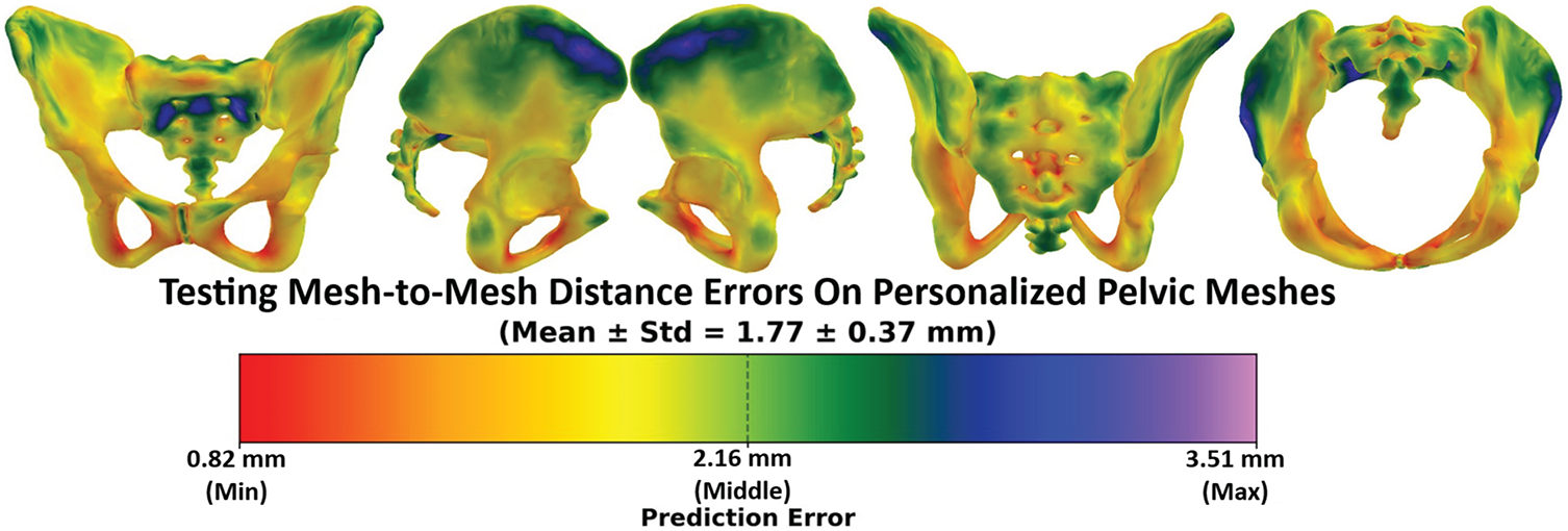
Figure 22: The testing mesh-to-mesh distance errors between the predicted pelvis bone meshes and the personalized pelvis bone meshes.

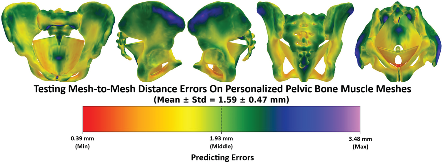
Figure 23: The testing mesh-to-mesh distance errors between the predicted pelvis bone & muscle meshes and the personalized pelvis bone and muscle meshes.

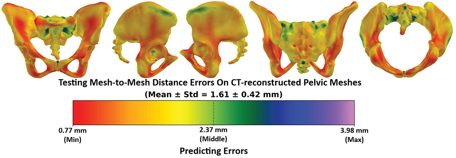
Figure 24: The testing mesh-to-mesh distance errors between the predicted pelvis bone meshes and the CT-reconstructed pelvis bone meshes.

3.6 Structural Alignment for the Best and Worst Predicted Cases

Fig. 25 illustrates the structural alignment between the predicted pelvic bone and muscle meshes (red) and the appropriate reference meshes (white). The comparisons were conducted with the personalized pelvic bone and muscle meshes and the CT-based pelvic bone mesh.

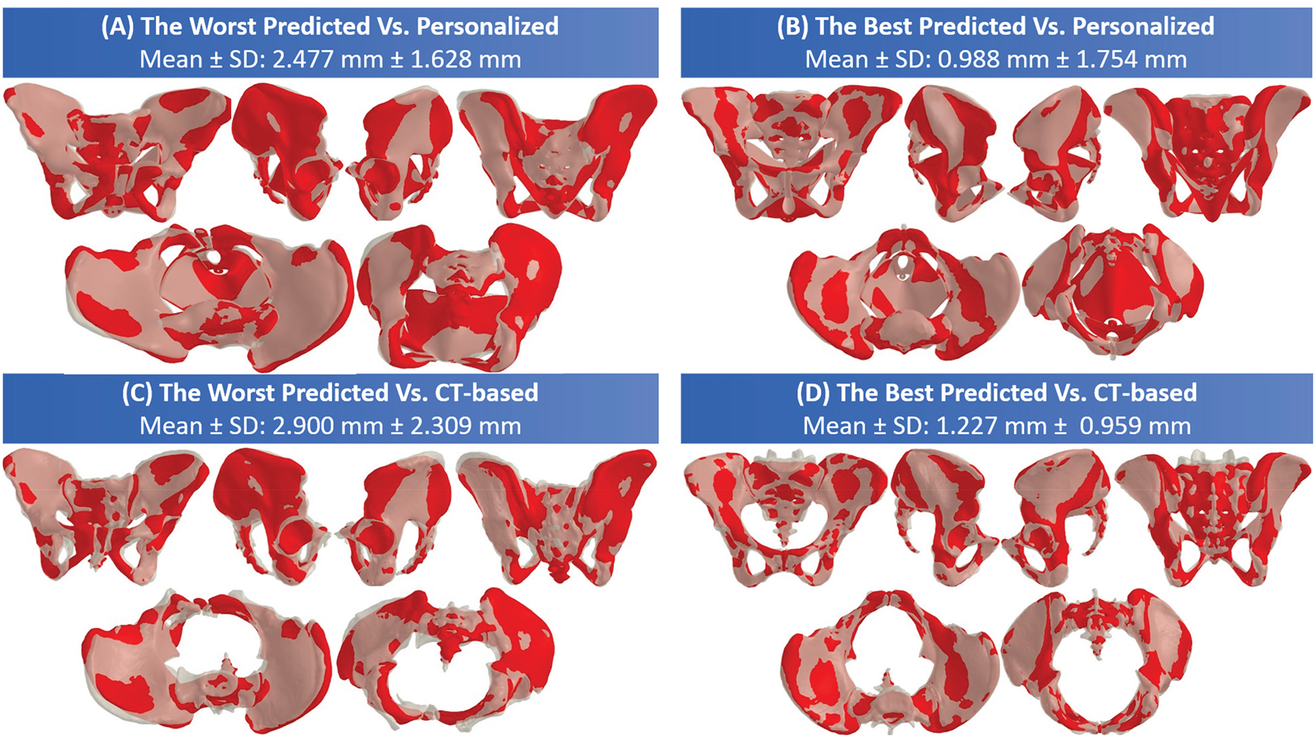
Figure 25: The structural alignment results for the best and worst predicted cases: (A) and (B) between the predicted pelvic bone muscle mesh (red) and the personalized pelvic bone muscle mesh (white); (C) and (D) between the predicted pelvic bone mesh (red) and the CT-based pelvic bone mesh (white).

Regarding the worst predicted case, the worst predicted cases (panels A and C) show significant misalignment between the predicted and personalized pelvic bone muscle mesh, with the vertex-to-surface distances of 2.447 ± 1.628 mm. The misalignment is also significantly apparent between the predicted and CT-based pelvic bone meshes, with the vertex-to-surface distances of 2.900 ± 2.309 mm. As shown in Fig. 22A,C, the misalignment most often occurs around complex anatomical regions like the iliac wings and pelvic floor. It is important to note that the CT-based pelvic bone in the worst predicted case is not symmetry and has outliers, as shown in Fig. 25C, so the SD error value when comparing with the CT-based bone mesh is 2.309 mm, which is larger than that when comparing with the personalized bone mesh, 1.628 mm. The high mean and SD values in the worst predicted case indicate that the prediction model struggles with abnormalities of the pelvic bone shape, such as irregular geometry, deformable regions, or incomplete feature correspondence.

Regarding the best predicted case, as shown in Fig. 25B,D, the predicted pelvic structure strongly overlaps with both personalized and CT-based pelvic bone meshes. In particular, the mean vertex-to-surface distances are 0.988 and 1.227 mm when compared to the personalized and CT-based pelvic structure, respectively. The SD value when compared with the personalized pelvic structure is 1.754 mm, which is higher than when compared with the CT-based pelvic structure. This is because the personalized pelvic structure has more pelvic muscles. Note that the mean error when compared to the CT-based pelvic structure is higher than when compared to the personalized pelvic structure due to the greater anatomical complexity.

Fig. 26 illustrates an example of multi-angle 3-D visualization of predicted pelvic bone and muscle structures predicted from the structural features picked from a DICOM image set. The predicted bone structure is well-aligned with the bone regions of the CT image slices. The predicted muscle structure can be personalized to the surrounding structures visualized in the CT image, as shown in Fig. 26A. Moreover, the predicted pelvic structures are also matched with the torso shape, as shown in Fig. 26B.

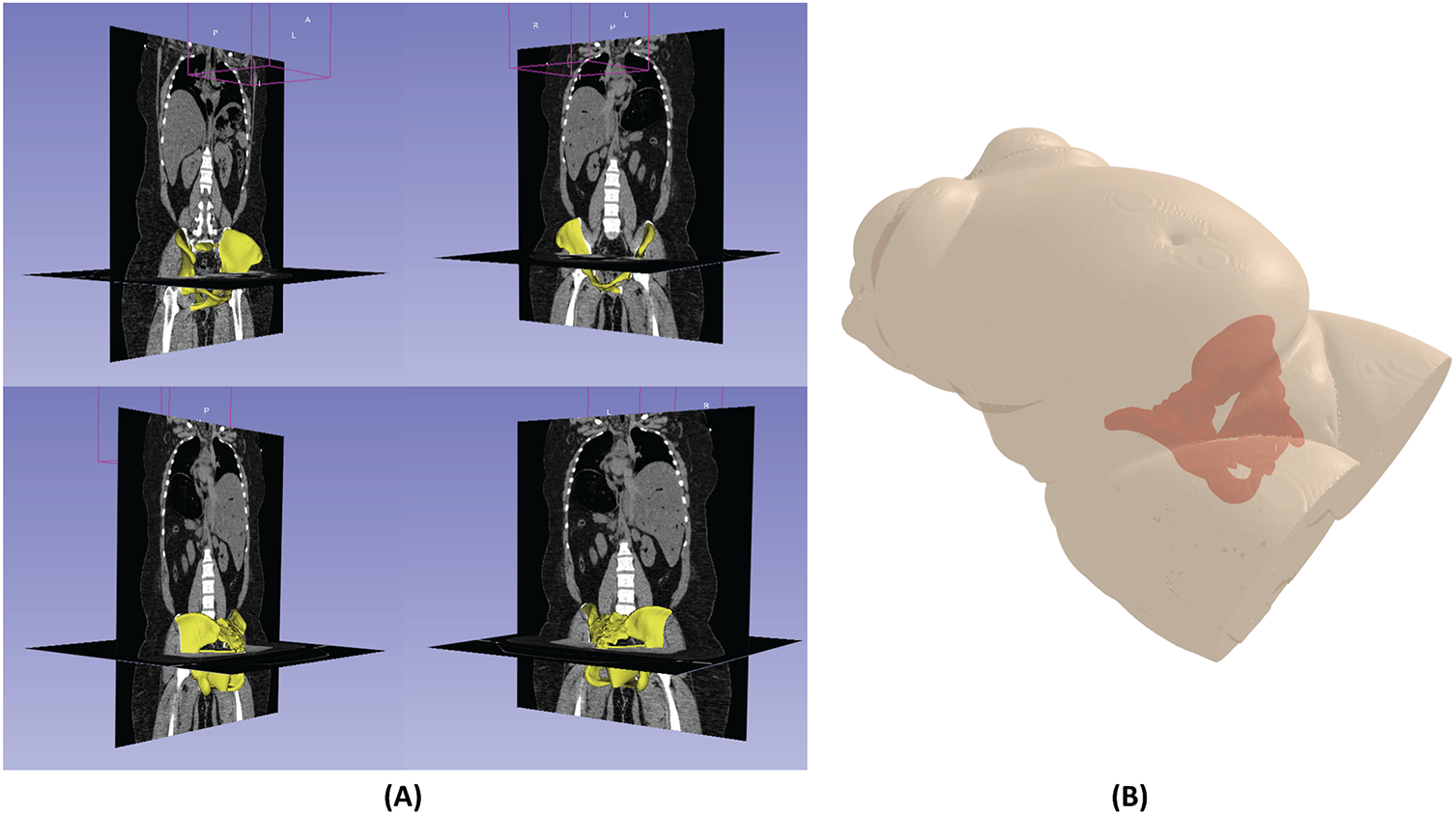
Figure 26: Multi-view 3-D visualization of predicted pelvic bone muscle structures overlaid on (A) axial and coronal DICOM slices and (B) 3-D torso structure. The yellow regions indicate the predicted pelvic bone and muscle structures.

4  Discussion

Fast and accurate prediction of the maternal pelvis and associated soft tissues plays an essential role in the translation of the computational childbirth model into clinical routine practices. Due to the geometrical complexities of these structures and tissues, current childbirth models use simplified geometries designed by using a computer-aided design approach [21,71]. The present study proposed a novel computational workflow to rapidly and accurately generate the personalized pelvis and associated soft tissue shapes from medical imaging. This study provides a way to perform personalized childbirth modeling and simulation for perineal tearing management. In fact, a population study can be suitably generated for enhancing the clinical findings and guidelines. In particular, we employed a novel statistical shape relation strategy to study the structural variations of the pelvis and associated soft tissues, leading to a prediction with an error level of 1.613 and 1.415 mm for the whole bone and muscle attachment regions, respectively. This prediction accuracy has never been achieved in the literature.

In addition to the clinical relevance, we addressed and achieved some technical challenges in this study: (1) a novel ROI pelvic structure personalization procedure; (2) a largest female pelvic dataset for biomechanical simulation of childbirth; (3) a novel statistical shape model of the whole pelvic structure; (4) a novel feature-to-structure pelvic reconstruction with a multiscale cross-validation.

(1) Regarding the first contribution, we introduced a coarse-to-fine procedure to personalize the template pelvic structure, including bone and muscle, to the target pelvic bone structure. In the coarse deformation stage, we personalized the template structure using a manually picked feature point set. This step initially minimizes the rigid differences between the template pelvic structure and the target pelvic structure. The affine transformation and non-rigid ICP methods were then sequentially applied to minimize non-rigid shape differences. Finally, the pelvic shape deformation was transferred to the pelvic bone and muscle with a radial basis function. In the fine deformation stage, each bone part of the coarse-deformed pelvis was adapted to the nearest geometries of the target pelvic bone. The rigid and non-rigid deformations of the template pelvic bone were transferred to the pelvic muscle using a radial basis function. Consequently, based only on the target pelvic bone mesh, we could personalize both the pelvic bone and muscle structure. In comparison with the rigid–elastic only approach, our proposed coarse-to-fine personalization procedure is better. One of the reasons relates to the use of a pipeline of rigid, affine, non-rigid ICP, Radial Basis Function with TPS, and ROI refinements to personalize the template pelvic structure to the target pelvic structure. This cascading process progressively reduced sources of discrepancies between the template and CT-based pelvic structures. In particular, the rigid SVD transformation first ensures global orientation and translation alignment. The affine (CPD) transformation then accounts for global scaling and shear differences. The non-rigid ICP transformation refines local vertex-level alignment while preserving anatomical plausibility. The RBF with TPS transformations propagates the pelvic shape deformation to the pelvic bone mesh. It also propagates bone mesh deformation to the muscle mesh. Finally, the ROI refinement strategy ensures local fidelity in critical regions such as sacroiliac joints and muscle attachments. While rigid—elastic can provide acceptable global alignment, it does not adequately handle scale differences or propagate deformations to internal muscle structures. Moreover, in comparison with previous studies, we personalized the template skull mesh to the target skull mesh based only on the deformation of the skull shape [72]. This shape-based deformation strategy cannot personalize the internal structure of the skull, so the region on the mandible jaw cannot be reconstructed accurately. In this study, as shown in Fig. 5, we first personalized the template pelvic shape to the target pelvic shape to initially align the anatomical features of the template pelvic bone to the target. Moreover, the initially aligned pelvic bone will be deformed to the target pelvic bone using local features and local pelvic structure. This procedure ensures the alignment of the internal structure of the pelvic bone. Note that some studies also tried to use a statistical shape model to personalize a template structure to the target structure. The personalization could be 2-D or 3-D to minimize shape differences by controlling the shape parameters [73–75]. However, this strategy is highly affected by the variability of the fitting data, and it cannot handle the complex geometrical structure of the target structure. Especially, most studies have conducted human shape personalization on the head [76,77], skull [78], femur [79], etc., but no studies have been conducted on shape personalization of the pelvic structure, particularly, including both bone and muscle structures. In this study, we first introduced the whole procedure for personalizing the template pelvic structure to the target pelvic structure. This procedure helps generate a dataset for developing shape models and geometrically analyzing the pelvic structure. Note that the accuracy of dataset preparation may be affected by manual anatomical landmark selection. This process can be labor-intensive and may introduce operator-dependent variability. However, in our study, the anatomical landmarks were only manually selected in the CT-based pelvic meshes for the initial registration of the template pelvic mesh to each CT-based mesh. After this initial step, our coarse-to-fine rigid and non-rigid registration pipeline, consisting of a cascade of complementary alignment methods, systematically eliminated global rigid differences and refined local non-rigid shape variations during pelvic structure personalization. Through this multi-stage optimization, the influence of subjective variability in the manually selected landmarks was substantially reduced, and the final personalized meshes were primarily determined by the automated registration algorithms rather than the initial manual inputs.

(2) Regarding the second contribution, we first generated a large scale of 300 female pelvic structures. This dataset has been anatomically aligned. This dataset can greatly support pelvic shape simulation and geometrical analyses. In the literature, previous pelvic datasets exist in the form of medical images, such as X-ray images [80], CT images [81], MRI images [82], pre-segmented DICOM [38], but no studies provide a pelvic dataset in the form of 3-D surface meshes, especially with a full set of bone and muscle structures of female subjects for childbirth simulation. The subject variability was indeed limited in ages, BME, or obstetric history. However, the two large and heterogeneous medical imaging datasets used in this study (NMDID and CTPelvic1K) capture substantial anatomical variability in pelvic morphology. Moreover, our objective focuses on methodological development rather than population-level anatomical characterization. The dataset preparation and shape learning pipeline introduced in this study can be easily scaled to additional subjects with richer demographic metadata. This can be conducted in future clinical collaborations.

(3) Regarding the third contribution, we first build a statistical shape model for the full pelvic structure, including bone and muscle. In a previous study, we identified a few studies that conduct modeling shape variation of the partial pelvic structures. Willemina et al., 2023 [83] built a PCA-based statistical shape model of the hemipelvis. However, this study did not fully model the whole structure of the pelvic bone and muscles, and the sample size of data was only 200 subjects. Additionally, the trained subjects were both males and females, not dedicated to female subjects like in this study. Consequently, our PCA model can be more accurate and flexible for simulating pelvic structures of female subjects in the application of childbirth simulation. The statistical shape model of the pelvic bone could also be found in the study of Praveen et al., 2022 [84], the authors simulated the shape variations of the hemipelvis for reconstructing the missing part of this pelvic part. However, only 33 female subjects were employed for fitting and testing, and not the whole pelvic structure can be simulated. The simulation of the full pelvic shape structure of female subjects brings benefits for several applications. In particular, the SSM of the whole pelvic structure can be used for simulating muscle-bone interactions, load-bearing, and movement dynamics in biomechanical modeling. Moreover, the pelvic SSM can also be used for modeling anatomical changes during pregnancy and delivery, and it is also useful for medical image analysis, surgical planning and simulation.

(4) Regarding the fourth contribution, we proposed a feature-to-structure pelvic structure reconstruction strategy based on the statistical shape relation coupled with multivariate regression. Shape relation could be represented as the relationship among the shape parameters, which are parameterized from the 3-D structure using a shape modeling method [30]. In a previous study, the shape relation was first analyzed among skull parts [85], between the head and skull shape [78], and between the front-head and back-head regions [86]. The skull part inter-relation could also be used for predicting the skull’s missing parts based on the skull’s existing parts [30]. The shape prediction errors among skull parts based on the shape relation can reach 1.32 to 2.54 mm, depending on the size of the predicted skull parts [30]. Based on the shape relation, the skull prediction errors could reach up to 2.696 mm [87]. With the shape relation, the skull missing part prediction errors could reach 0.21 to 0.54 mm according to the size of the missing part [30]. The back-head shape could also be predicted from the face-head shape with an error of 1.15 ± 0.21 mm [86]. In addition to the head and skull structures, the shape relation has not been analyzed on other human structures, such as the pelvic bone and meshes, and their structural features. In this study, we analyzed the relationship between the structural feature shape and the pelvic structure shape. Throughout a multiscale cross-validation process, we proved that the shape relation-based strategy is optimal for the issue of feature-to-pelvic structure reconstruction. Moreover, we also found that the shape parameters have inter-relationships, as the optimal multivariate regression was the multi-output with ridge regression. When compared to the CT-reconstructed pelvic meshes, the best and worst predicted errors were 1.227 ± 0.959 mm and 2.900 ± 2.309 mm, respectively. These errors are compatible with the shape prediction strategy for the skull part inter-relation, head-to-skull relation, and face-head-to-back-head prediction.

The prediction of whole pelvic structures from structural features has valuable applications across several fields. In medical and clinical applications, this procedure can provide accurate anatomical structure in the case of trauma or deformities. Moreover, it can reconstruct high-resolution pelvic structures based only on feature points in a low-quality medical image. In the fields of biomechanics and robotics, this strategy can help personalize the full pelvic structure based only on externally selected feature points on the target body for fast simulation of childbirth and motion analyses. The strategy can help predict the missing part of the pelvic structures based only on feature points and/or existing parts. Note that previous studies reported that clinically acceptable surface errors for pelvic bones typically fall within 1–2 mm. However, more complex regions, such as the ischium or pelvic floor, may tolerate 2–5 mm deviations [88,89]. Our best and worst prediction errors were 1.227 ± 0.959 mm and 2.900 ± 2.309 mm, respectively, which are within the acceptable range of the pelvic structure prediction accuracy. In comparison with deep learning-based pelvic segmentation methods, such as 2D/3D U-Net [90,91], fully convolution network [92], multi-scale and pyramid CNNs [93], the accuracy of bladder and prostate segmentation could reach a DSC of 0.90–0.96 (~ 1–3 mm for surface error). The rectum and pelvic floor muscle segmentation generally ranges from a DSC of 0.65–0.8 (~ 3–5 mm). Our mesh-to-mesh errors were compatible with the reported errors in these deep learning-based segmentations. However, our method predicts complete 3-D pelvic structures from sparse structural features. This approach is different from the voxel segmentation in deep learning-based segmentation. However, our procedure has not been validated in clinical environments for evaluating the clinical outcomes, such as perineal tearing severity. Our acceptable accuracy in this study could be a necessary first step toward future biomechanical simulations in clinical applications.

However, this study still has some limitations related to the diversity of the dataset, the employed shape modeling technique, and the lack of ground truth muscle structures. Regarding dataset diversity, in this study, the selected subjects were from America only. As a targeted childbirth simulation, only 300 adult female subjects were employed to fit and evaluate the feature-to-pelvic reconstruction. Due to the small quantity of subjects in the dataset, we could only employ the PCA-based statistical shape modeling methods to illustrate the shape variation of the pelvic structures. This shape modeling method limits the range of shape variation, so we could not accurately reconstruct some regions of the pelvic structure with complex geometries. Moreover, in this study, the muscle structure was manually designed using CAD software, so the actual geometrical structure of the pelvic muscle was simplified. The personalization of the muscle structure was based only on the non-rigid deformation of the muscle attachment points, not on the shape variation of the real pelvic muscles. In perspective, we will increase the variability of the pelvic structure dataset both quantitatively and qualitatively. More pelvic structures from the European and Asian countries will be collected. When obtaining a larger dataset, we will employ the neural shape network [94] for handling the pelvic geometrical complexity more efficiently. Additionally, our study used publicly available CT datasets, which do not include obstetric information such as parity, fetal size, or delivery outcomes. Consequently, we could not analyze the model performance specifically in high-risk groups. In further research, we plan to extend the pipeline to clinically annotated datasets once such data become available. Finally, the shape of the pelvic muscles will be reconstructed from MRI images to estimate the shape variation of the pelvic muscle structures more accurately. We will also implement and test the developed feature-to-pelvic structure pipeline into a graphical user interface (GUI) to enable fast reconstruction of the entire pelvic structure from manually selected feature points.

5  Conclusion

This study proposes, for the first time, a fast prediction method of 3D complex female pelvis and associated soft tissue shapes using a novel statistical shape relation strategy. The obtained results showed accurate predictions with errors of 1.613 mm and 1.415 mm for the whole bone and muscle attachment regions, respectively. This study provides a way to perform personalized childbirth modeling and simulation for perineal tearing management. The present work’s perspectives relate to the application of the proposed approach to childbirth MRI data for fast model generation. The implementation of a graphical user interface facilitating the model generation process will be investigated and evaluated.

Acknowledgement: Not applicable.

Funding Statement: This research is funded by Vietnam National University Ho Chi Minh City (VNU-HCM) under grant number DS.C2025-28-06.

Author Contributions: The authors confirm contribution to the paper as follows: Conceptualization, Tien-Tuan Dao and Tan-Nhu Nguyen; methodology, Tan-Nhu Nguyen; validation, Tan-Nhu Nguyen; formal analysis, Tien-Tuan Dao; investigation, Tan-Nhu Nguyen; data curation, Trong-Pham Nguyen-Huu; writing—original draft preparation, Tan-Nhu Nguyen; writing—review and editing, Tan-Nhu Nguyen and Tien-Tuan Dao; visualization, Tan-Nhu Nguyen and Trong-Pham Nguyen-Huu; supervision, Tien-Tuan Dao; project administration, Tan-Nhu Nguyen; funding acquisition, Tan-Nhu Nguyen. All authors reviewed and approved the final version of the manuscript.

Availability of Data and Materials: The data that support the findings of this study are openly available in a GitHub Repository at https://github.com/TanNhuNguyen/FeatureBasedPelvisReconstruction.

Ethics Approval: Not applicable.

Conflicts of Interest: The authors declare no conflicts of interest.

Appendix A The Pseudocode of the Pelvic Structure Personalization Procedure

The pseudocode of the pelvic structure personalization procedure is presented in Algorithm A1. In particular, the inputs of this procedure are the template pelvic meshes (bone, muscle, coarse pelvic shape, and the ROI meshes), the template anatomical landmarks coupled with their barycentric coordinates, and the target pelvis meshes coupled with their anatomical landmarks for all subjects. The outputs of this procedure are the personalized pelvic bone-muscle mesh for each subject. The procedure first loads the template pelvic meshes, including coarse shape, full bone-muscle mesh, bone mesh, muscle mesh, and other ROI meshes (left ilium, right ilium, sacrum, and joints). The template anatomical landmarks are also loaded and used for computing their barycentric coordinates on the template pelvic shape and on the template pelvic bone mesh. Moreover, the vertex index mappings from the ROI meshes to the full pelvic mesh are also computed first. For each subject in the dataset, give the main stages: (1) Global Alignment with Template Shape, (2) Whole-mesh Deformation, (3) ROI-based Local Refinement, (4) Muscle Personalization, and (5) Output Saving. In Stage 1: Global Alignment with the Target Pelvic Shape, the target pelvic shape, bone mesh, and its anatomical landmarks are first loaded. The aligned pelvic shape, that is the output aligned pelvic shape in Stage 1, is initialized with the template pelvic shape. The aligned pelvic shape is then transformed using the SVD registration from the template anatomical landmarks to the target anatomical landmarks. The landmarks of the aligned pelvic shape are also updated using the barycentric coordinate on the template pelvic shape. An affine transform is also estimated from the aligned pelvic landmarks to the target landmarks before being applied to the aligned pelvic shape. The non-rigid ICP deforms the aligned pelvic shape toward the target pelvic shape, constrained by their barycentric landmarks. Finally, the deformed aligned pelvic shape is projected on the target pelvic shape. In Stage 2: Whole-Mesh Deformation, the deformed pelvic shape and the deformed pelvic bone-muscle mesh are initialized with the template pelvic shape and the template pelvic bone-muscle mesh, respectively. The rigid SVD and CPD affine registration are then applied to the deformed pelvic shape and the deformed pelvic bone-muscle mesh to move and scale the shape to the target pelvic shape based on the anatomical landmarks. The vertex displacements from the registered deformed pelvic shape to the aligned pelvic shape, which is the output from Stage 1, are computed before propagating to the deformed pelvic bone-muscle vertices. The outputs of this stage are the deformed pelvic bone-muscle mesh. In Stage 3: ROI-Based Local Refinement, the ROI meshes are extracted from the deformed pelvic bone-muscle mesh using the ROI vertex index mappings. The anatomical landmarks on each ROI mesh are also reconstructed using the barycentric coordinates on the ROI mesh. The target ROI anatomical landmarks are also extracted. The non-rigid ICP registration with TPS deforms each ROI mesh to its target ROI mesh with the constraints of its ROI anatomical landmarks. Each vertex of the deformed pelvic bone-muscle mesh from Stage 2 is replaced with the vertices of the deformed ROI meshes using their ROI vertex index mappings. The output of this stage is the personalized pelvic bone-muscle mesh. In Stage 4: Muscle Personalization, the initial pelvic muscle mesh is formed from the deformed pelvic bone-muscle mesh from Stage 2 using its vertex index mapping. The deformed and personalized muscle feature points were reconstructed using their barycentric coordinates on the deformed and personalized pelvic bone mesh. Note that the deformed pelvic bones mesh formed from the vertices of the deformed pelvic bone-muscle mesh from Stage 2 using its vertex index mapping, and the personalized pelvic bone mesh is formed from the personalized pelvic bone-muscle mesh from Stage 3 using its vertex index mapping. The 3-D displacements from the deformed to personalized muscle feature points are propagated to the muscle vertices to form the personalized muscle mesh.

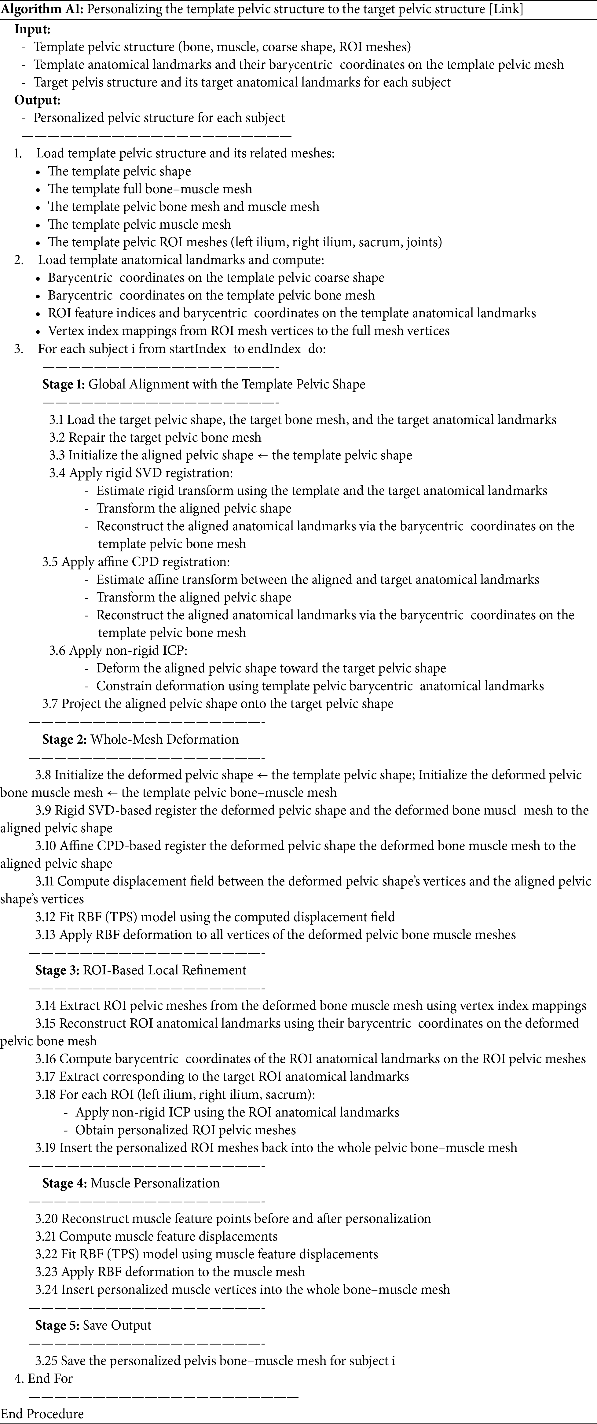
Appendix B The Pseudocode for Reconstructing Pelvic Structures from Structural Features Using the Affine Transform-Based Non-Rigid Deformation

Appendix C The Pseudocode for Reconstructing Pelvic Structures from Structural Features Using the Radial Basis Function-Based Non-Rigid Deformation

Appendix D The Pseudocode for Reconstructing Pelvic Structures from Structural Features Using Statistical Shape Optimization

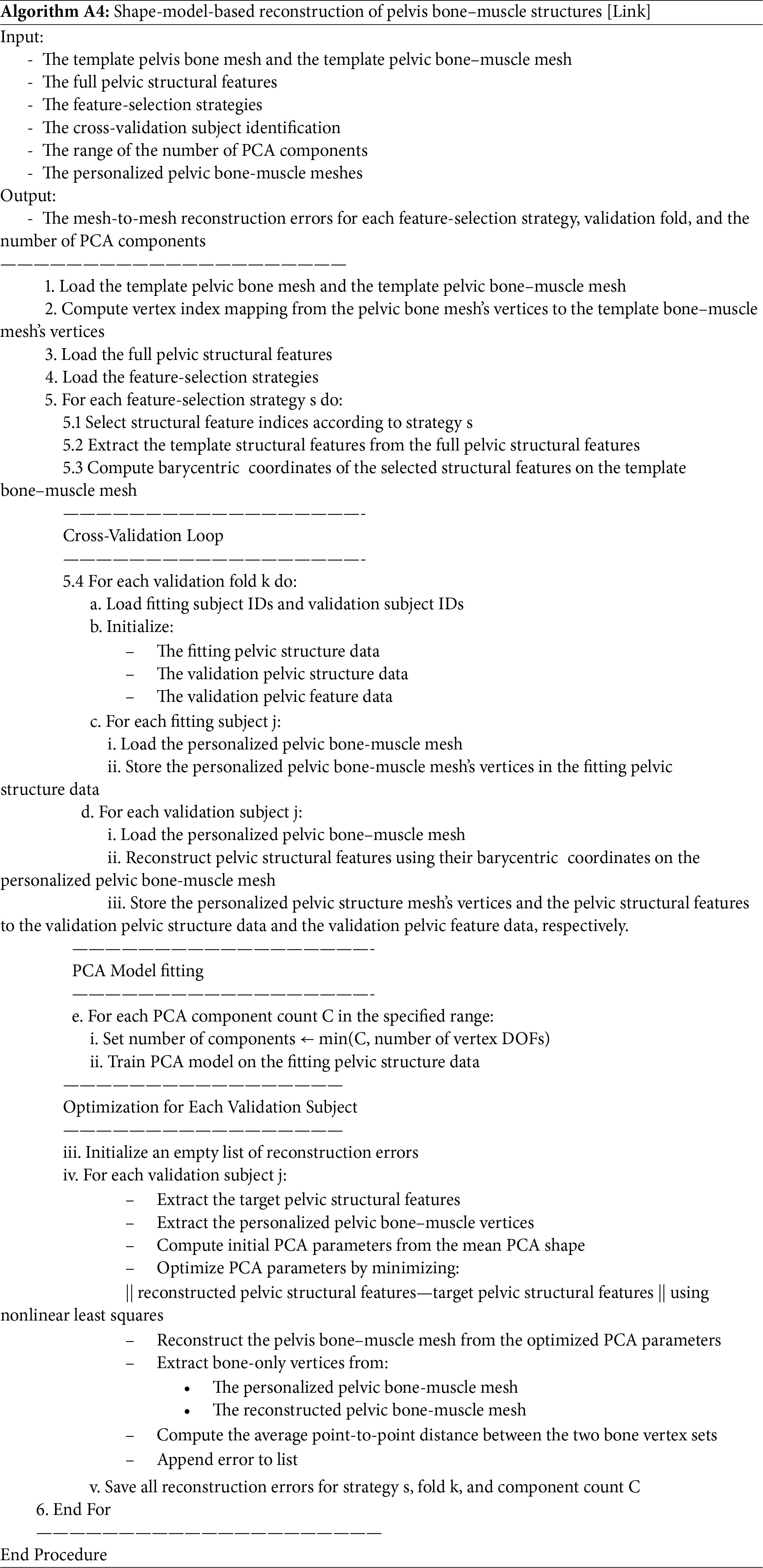
Appendix E The Pseudocode for Reconstructing Pelvic Structures from Structural Features Using the Shape Relation-Based Prediction

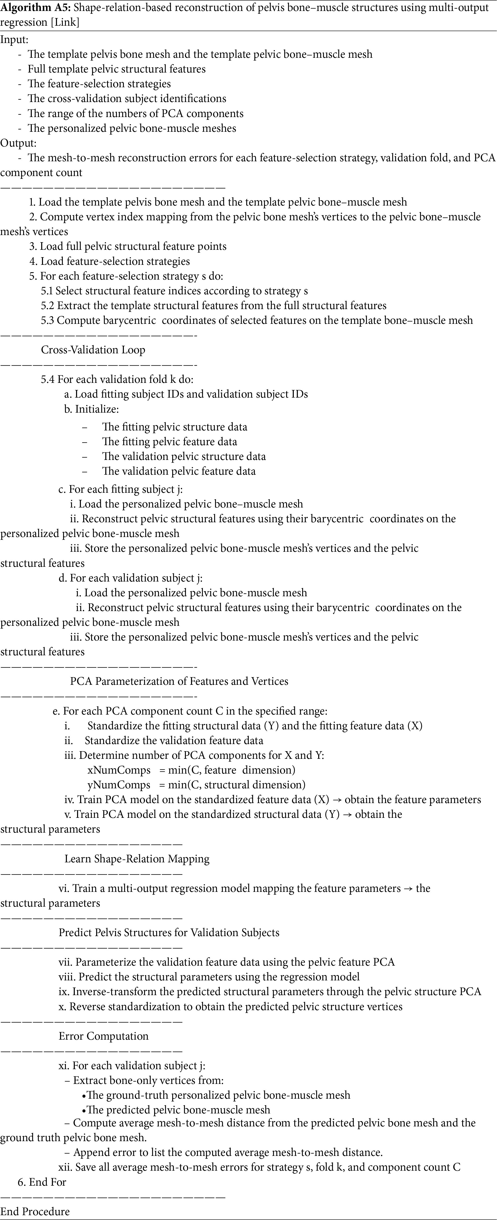
References

1. Okeahialam NA, Sultan AH, Thakar R. The prevention of perineal trauma during vaginal birth. Am J Obstet Gynecol. 2024;230(3):S991–1004. doi:10.1016/j.ajog.2022.06.021. [Google Scholar] [CrossRef]

2. Abedzadeh-Kalahroudi M, Talebian A, Sadat Z, Mesdaghinia E. Perineal trauma: incidence and its risk factors. J Obstet Gynaecol. 2019;39(2):206–11. doi:10.1080/01443615.2018.1476473. [Google Scholar] [CrossRef]

3. Ducarme G, Pizzoferrato AC, de Tayrac R, Schantz C, Thubert T, Le Ray C, et al. Perineal prevention and protection in obstetrics: CNGOF clinical practice guidelines. J Gynecol Obstet Hum Reprod. 2019;48(7):455–60. doi:10.1016/j.jogoh.2018.12.002. [Google Scholar] [CrossRef]

4. Schmidt PC, Fenner DE. Repair of episiotomy and obstetrical perineal lacerations (first-fourth). Am J Obstet Gynecol. 2024;230(3):S1005–13. doi:10.1016/j.ajog.2022.07.005. [Google Scholar] [CrossRef]

5. Frohlich J, Kettle C. Perineal care. BMJ Clin Evid. 2015;2015:1401. [Google Scholar]

6. Saucedo AM, Tuuli MG, Gregory WT, Richter HE, Lowder JL, Woolfolk C, et al. First and second stage risk factors associated with perineal lacerations. Matern Child Health J. 2024;28(7):1228–33. doi:10.1007/s10995-024-03919-1. [Google Scholar] [CrossRef]

7. Sultan AH, Kamm MA, Hudson CN, Bartram CI. Third degree obstetric anal sphincter tears: risk factors and outcome of primary repair. Bmj. 1994;308(6933):887–91. doi:10.1136/bmj.308.6933.887. [Google Scholar] [CrossRef]

8. Gachon B, Fritel X, Pierre F, Nordez A. In vivo assessment of the elastic properties of women’s pelvic floor during pregnancy using shear wave elastography: design and protocol of the ELASTOPELV study. BMC Musculoskelet Disord. 2020;21(1):305. doi:10.1186/s12891-020-03333-y. [Google Scholar] [CrossRef]

9. Hoyte L, Schierlitz L, Zou K, Flesh G, Fielding JR. Two- and 3-dimensional MRI comparison of levator ani structure, volume, and integrity in women with stress incontinence and prolapse. Am J Obstet Gynecol. 2001;185(1):11–9. doi:10.1067/mob.2001.116365. [Google Scholar] [CrossRef]

10. Kruger JA, Heap SW, Murphy BA, Dietz HP. Pelvic floor function in nulliparous women using three-dimensional ultrasound and magnetic resonance imaging. Obstet Gynecol. 2008;111(3):631–8. doi:10.1097/aog.0b013e3181655dc2. [Google Scholar] [CrossRef]

11. Barbaric ZL, Marumoto AK, Raz S. Magnetic resonance imaging of the perineum and pelvic floor. Top Magn Reson Imag. 2001;12(2):83–92. doi:10.1097/00002142-200104000-00002. [Google Scholar] [CrossRef]

12. Lallemant M, Kadiakhe T, Chambert J, Lejeune A, Ramanah R, Mottet N, et al. In vitro biomechanical properties of porcine perineal tissues to better understand human perineal tears during delivery. Acta Obstet Gynecol Scand. 2024;103(7):1386–95. doi:10.1111/aogs.14791. [Google Scholar] [CrossRef]

13. Kadiaké T, Lallemant M, Chambert J, Mottet N, Lejeune A, Jacquet E. Towards the biomechanical modelling of the behaviour of ex-vivo porcine perineal tissues. J Biomech. 2024;171:112175. doi:10.1016/j.jbiomech.2024.112175. [Google Scholar] [CrossRef]

14. Moura R, Oliveira DA, Parente MPL, Kimmich N, Natal Jorge RM. A biomechanical perspective on perineal injuries during childbirth. Comput Meth Programs Biomed. 2024;243:107874. doi:10.1016/j.cmpb.2023.107874. [Google Scholar] [CrossRef]

15. Lien KC, Mooney B, DeLancey JOL, Ashton-Miller JA. Levator ani muscle stretch induced by simulated vaginal birth. Obstet Gynecol. 2004;103(1):31–40. doi:10.1097/01.aog.0000109207.22354.65. [Google Scholar] [CrossRef]

16. Moura R, Oliveira DA, Ferreira JPS, Parente MPL, Kimmich N, Natal Jorge RM. A finite element-based machine learning framework to predict the mechanical behavior of the pelvic floor muscles during childbirth. Expert Syst Appl. 2024;250:123953. doi:10.1016/j.eswa.2024.123953. [Google Scholar] [CrossRef]

17. Rao GV, Rubod C, Brieu M, Bhatnagar N, Cosson M. Experiments and finite element modelling for the study of prolapse in the pelvic floor system. Comput Meth Biomech Biomed Eng. 2010;13(3):349–57. doi:10.1080/10255840903251270. [Google Scholar] [CrossRef]

18. Xu Z, Chen N, Wang B, Yang J, Liu H, Zhang X, et al. Creation of the biomechanical finite element model of female pelvic floor supporting structure based on thin-sectional high-resolution anatomical images. J Biomech. 2023;146:111399. doi:10.1016/j.jbiomech.2022.111399. [Google Scholar] [CrossRef]

19. Moura R, Oliveira DA, Parente MPL, Kimmich N, Hynčík L, Hympánová LH, et al. Patient-specific surrogate model to predict pelvic floor dynamics during vaginal delivery. J Mech Behav Biomed Mater. 2024;160:106736. doi:10.1016/j.jmbbm.2024.106736. [Google Scholar] [CrossRef]

20. Nguyen TNT, Ballit A, Ferrandini M, Colliat JB, Dao TT. Fetus descent simulation with the active uterine contraction during the vaginal delivery: MRI-based evaluation and uncertainty quantification. Comput Meth Biomech Biomed Eng. 2024:1–16. doi:10.1080/10255842.2024.2399777. [Google Scholar] [CrossRef]

21. Chen S, Grimm MJ. Childbirth computational models: characteristics and applications. J Biomech Eng. 2021;143(5):050801. doi:10.1115/1.4049226. [Google Scholar] [CrossRef]

22. Badaoui S, Grevent D, Salomon LJ, Ville Y, Stirnemann J. Magnetic resonance imaging-based three-dimensional modeling of pregnant pelvis for fetoscopic surgical planning. Ultrasound Obs Gyne. 2020;56(5):793–5. doi:10.1002/uog.22067. [Google Scholar] [CrossRef]

23. Moura R, Oliveira DA, Kimmich N, Jorge RMN, Parente MPL. Computational modeling of vacuum-assisted delivery: biomechanics of maternal soft tissues. Biomech Model Mechanobiol. 2025;24(4):1435–46. doi:10.1007/s10237-025-01977-0. [Google Scholar] [CrossRef]

24. Gaffney BMM, Hillen TJ, Nepple JJ, Clohisy JC, Harris MD. Statistical shape modeling of femur shape variability in female patients with hip dysplasia. J Orthop Res. 2019;37(3):665–73. doi:10.1002/jor.24214. [Google Scholar] [CrossRef]

25. Devismes-Ferrandini M, Nguyen TN, Dao TT. From clinical measurements to articulated foetus: statistical shape modeling of bone contours using PLSR for enhanced childbirth simulation. Comput Meth Programs Biomed. 2025;270:108934. doi:10.1016/j.cmpb.2025.108934. [Google Scholar] [CrossRef]

26. Lu Y, Wang X, Yang B, Xu Z, Zhang B, Jia B, et al. Application of SolidWorks software in preoperative planning of high tibial osteotomy. Front Surg. 2023;9:951820. doi:10.3389/fsurg.2022.951820. [Google Scholar] [CrossRef]

27. Antoine Maintz JB, Viergever MA. A survey of medical image registration. Med Image Anal. 1998;2(1):1–36. doi:10.1016/s1361-8415(01)80026-8. [Google Scholar] [CrossRef]

28. Hillier M. Radial basis functions. Cham, Switzerland: Springer International Publishing; 2023. p. 1175–82. doi:10.1007/978-3-030-85040-1_263. [Google Scholar] [CrossRef]

29. Heitz G, Rohlfing T, Maurer CR Jr. Statistical shape model generation using nonrigid deformation of a template mesh. In: Fitzpatrick JM, Reinhardt JM, editors. Medical imaging 2005: image processing. San Diego, CA, USA: SPIE; 2005. 1411 p. doi:10.1117/12.594802. [Google Scholar] [CrossRef]

30. Nguyen TN, Vo PP, Tran VD, Nguyen HN, Pham HA, Le-Ngoc HA, et al. Novel shape learning and prediction for skull part completion and reconstruction. Vis Comput. 2025;41(11):8873–93. doi:10.1007/s00371-025-03904-x. [Google Scholar] [CrossRef]

31. Maggino F, Fattore M. Multivariate statistical analysis. In: Encyclopedia of quality of life and well-being research. Dordrecht, The Netherlands: Springer; 2014. p. 4223–8. doi:10.1007/978-94-007-0753-5_1890. [Google Scholar] [CrossRef]

32. Tirink C, Abaci SH, Onder H. Comparison of ridge regression and least squares methods in the presence of multicollinearity for body measurements in Saanen kids. Iğdır Üniversitesi Fen Bilim Enstitüsü Derg. 2020;10(2):1429–37. doi:10.21597/jist.671662. [Google Scholar] [CrossRef]

33. Uurtio V, Monteiro JM, Kandola J, Shawe-Taylor J, Fernandez-Reyes D, Rousu J. A tutorial on canonical correlation methods. ACM Comput Surv. 2018;50(6):1–33. doi:10.1145/3136624. [Google Scholar] [CrossRef]

34. Indahl UG, Liland KH, Næs T. Canonical partial least squares—a unified PLS approach to classification and regression problems. J Chemom. 2009;23(9):495–504. doi:10.1002/cem.1243. [Google Scholar] [CrossRef]

35. Rasmussen CE. Gaussian processes in machine learning. In: Advanced lectures on machine learning. Berlin/Heidelberg, Germany: Springer; 2004. p. 63–71. doi:10.1007/978-3-540-28650-9_4. [Google Scholar] [CrossRef]

36. Borchani H, Varando G, Bielza C, Larrañaga P. A survey on multi-output regression. WIREs Data Min Knowl. 2015;5(5):216–33. doi:10.1002/widm.1157. [Google Scholar] [CrossRef]

37. Berry SD, Edgar HJ. A new resource for pathology informatics: the New Mexico decedent image database. J Pathol Inform. 2021;12(1):44. doi:10.4103/2153-3539.330157. [Google Scholar] [CrossRef]

38. Liu P, Han H, Du Y, Zhu H, Li Y, Gu F, et al. Deep learning to segment pelvic bones: large-scale CT datasets and baseline models. Int J Comput Assist Radiol Surg. 2021;16(5):749–56. doi:10.1007/s11548-021-02363-8. [Google Scholar] [CrossRef]

39. Shen C, Wang P, Roth HR, Yang D, Xu D, Oda M, et al. Multi-task federated learning for heterogeneous pancreas segmentation. Cham, Switzerland: Springer International Publishing; 2021. [Google Scholar]

40. Simpson AL, Antonelli M, Bakas S, Bilello M, Farahani K, van Ginneken B, et al. A large annotated medical image dataset for the development and evaluation of segmentation algorithms. arXiv:1902.09063. 2019. [Google Scholar]

41. Heller N, Isensee F, Maier-Hein KH, Hou X, Xie C, Li F, et al. The state of the art in kidney and kidney tumor segmentation in contrast-enhanced CT imaging: results of the KiTS19 challenge. Med Image Anal. 2021;67(1):101821. doi:10.1016/j.media.2020.101821. [Google Scholar] [CrossRef]

42. Ju F, Wu Y, Dong M, Zhao J. MiFDeU: multi-information fusion network based on dual-encoder for pelvic bones segmentation. Eng Appl Artif Intell. 2025;147:110230. doi:10.1016/j.engappai.2025.110230. [Google Scholar] [CrossRef]

43. Papoutsoglou M, Kapitsaki GM, German D, Angelis L. An analysis of open source software licensing questions in Stack Exchange sites. J Syst Softw. 2022;183:111113. doi:10.1016/j.jss.2021.111113. [Google Scholar] [CrossRef]

44. Amla Z, Khehra PS, Mathialagan A, Lugez E. Review of the free research software for computer-assisted interventions. J Imag Inform Med. 2024;37(1):386–401. doi:10.1007/s10278-023-00912-y. [Google Scholar] [CrossRef]

45. Newman TS, Yi H. A survey of the marching cubes algorithm. Comput Graph. 2006;30(5):854–79. doi:10.1016/j.cag.2006.07.021. [Google Scholar] [CrossRef]

46. Praschl C, Krauss O. Extending 3D geometric file formats for geospatial applications. Appl Geomat. 2024;16(1):161–80. doi:10.1007/s12518-023-00543-6. [Google Scholar] [CrossRef]

47. Kurmis AP. Gender differences in unintended anterior pelvic roll during primary THA in the lateral position. J Orthop Surg Res. 2024;19(1):419. doi:10.1186/s13018-024-04811-y. [Google Scholar] [CrossRef]

48. Lewis CL, Laudicina NM, Khuu A, Loverro KL. The human pelvis: variation in structure and function during gait. Anat Rec. 2017;300(4):633–42. doi:10.1002/ar.23552. [Google Scholar] [CrossRef]

49. Gasparutto X, Besonhe P, DiGiovanni PL, Zingg M, Boudabbous S, Armand S, et al. Reliability of the pelvis and femur anatomical landmarks and geometry with the EOS system before and after total hip arthroplasty. Sci Rep. 2022;12(1):21420. doi:10.1038/s41598-022-25997-3. [Google Scholar] [CrossRef]

50. Gold M, Munjal A, Varacallo MA. Anatomy, bony pelvis and lower limb, hip joint. Treasure Island, FL, USA: StatPearls Publishing; 2025. [Google Scholar]

51. Burgess MD, Lui F. Anatomy, bony pelvis and lower limb: pelvic bones. Treasure Island, FL, USA: StatPearls Publishing; 2025. [Google Scholar]

52. Chaudhry SR, Nahian A, Chaudhry K. Anatomy, abdomen and pelvis, pelvis. Treasure Island, FL, USA: StatPearls Publishing; 2025. [Google Scholar]

53. Roch M, Gaudreault N, Cyr MP, Venne G, Bureau NJ, Morin M. The female pelvic floor Fascia Anatomy: a systematic search and review. Life. 2021;11(9):900. doi:10.3390/life11090900. [Google Scholar] [CrossRef]

54. Siccardi MA, Valle C. Anatomy, bony pelvis and lower limb: pelvic fascia. Treasure Island, FL, USA: StatPearls Publishing; 2025. [Google Scholar]

55. Eickmeyer SM. Anatomy and physiology of the pelvic floor. Phys Med Rehabil Clin N Am. 2017;28(3):455–60. doi:10.1016/j.pmr.2017.03.003. [Google Scholar] [CrossRef]

56. Herschorn S. Female pelvic floor anatomy: the pelvic floor, supporting structures, and pelvic organs. Rev Urol. 2004;6(Suppl 5):S2–10. [Google Scholar]

57. Chen WM, Cai YH, Yu Y, Geng X, Ma X. Optimal mesh criteria in finite element modeling of human foot: the dependence for multiple model outputs on mesh density and loading boundary conditions. J Mech Med Biol. 2021;21(9):2140034. doi:10.1142/s0219519421400340. [Google Scholar] [CrossRef]

58. Veilleux NJ, Kalore NV, Vossen JA, Wayne JS. Automatic characterization of pelvic and sacral measures from 200 subjects. J Bone Jt Surg. 2020;102(23):e130. doi:10.2106/jbjs.20.00343. [Google Scholar] [CrossRef]

59. Wang RY, Xu WH, Kong XC, Yang L, Yang SH. Measurement of acetabular inclination and anteversion via CT generated 3D pelvic model. BMC Musculoskelet Disord. 2017;18(1):373. doi:10.1186/s12891-017-1714-y. [Google Scholar] [CrossRef]

60. Arand C, Wagner D, Richards RG, Noser H, Kamer L, Sawaguchi T, et al. 3D statistical model of the pelvic ring-a CT-based statistical evaluation of anatomical variation. J Anat. 2019;234(3):376–83. doi:10.1111/joa.12928. [Google Scholar] [CrossRef]

61. Hêches J, Marcadent S, Fernandez A, Adjahou S, Meuwly JY, Thiran JP, et al. Accuracy and reliability of pelvimetry measures obtained by manual or automatic labeling of three-dimensional pelvic models. J Clin Med. 2024;13(3):689. doi:10.3390/jcm13030689. [Google Scholar] [CrossRef]

62. Arun KS, Huang TS, Blostein SD. Least-squares fitting of two 3-D point sets. IEEE Trans Pattern Anal Mach Intell. 1987;5:698–700. doi:10.1109/tpami.1987.4767965. [Google Scholar] [CrossRef]

63. Myronenko A, Song X. Point set registration: coherent point drift. IEEE Trans Pattern Anal Mach Intell. 2010;32(12):2262–75. doi:10.1109/tpami.2010.46. [Google Scholar] [CrossRef]

64. Amberg B, Romdhani S, Vetter T. Optimal step nonrigid ICP algorithms for surface registration. In: Proceedings of the 2007 IEEE Conference on Computer Vision and Pattern Recognition; 2007 Jun 17–22; Minneapolis, MN, USA. p. 1–8. doi:10.1109/cvpr.2007.383165. [Google Scholar] [CrossRef]

65. Keller W, Borkowski A. Thin plate spline interpolation. J Geod. 2019;93(9):1251–69. doi:10.1007/s00190-019-01240-2. [Google Scholar] [CrossRef]

66. Virtanen P, Gommers R, Oliphant TE, Haberland M, Reddy T, Cournapeau D, et al. SciPy 1.0: fundamental algorithms for scientific computing in Python. Nat Methods. 2020;17(3):261–72. doi:10.1038/s41592-019-0686-2. [Google Scholar] [CrossRef]

67. Warren J, Schaefer S, Hirani AN, Desbrun M. Barycentric coordinates for convex sets. Adv Comput Math. 2007;27(3):319–38. doi:10.1007/s10444-005-9008-6. [Google Scholar] [CrossRef]

68. Bentley JL. Multidimensional binary search trees used for associative searching. Commun ACM. 1975;18(9):509–17. doi:10.1145/361002.361007. [Google Scholar] [CrossRef]

69. Richards LE, Jolliffe IT. Principal component analysis. J Mark Res. 1988;25(4):410. doi:10.2307/3172953. [Google Scholar] [CrossRef]

70. Aksu G, Güzeller CO, Eser MT. The effect of the normalization method used in different sample sizes on the success of artificial neural network model. Int J Assess Tools Educ. 2019;6(2):170–92. doi:10.21449/ijate.479404. [Google Scholar] [CrossRef]

71. Lapeer R, Gerikhanov Z, Sadulaev SM, Audinis V, Rowland R, Crozier K, et al. A computer-based simulation of childbirth using the partial Dirichlet–Neumann contact method with total Lagrangian explicit dynamics on the GPU. Biomech Model Mechanobiol. 2019;18(3):681–700. doi:10.1007/s10237-018-01109-x. [Google Scholar] [CrossRef]

72. Nguyen TN, Ballit A, Dao TT. A novel stereo camera fusion scheme for generating and tracking real-time 3-D patient-specific head/face kinematics and facial muscle movements. IEEE Sens J. 2023;23(9):9889–97. doi:10.1109/jsen.2023.3259473. [Google Scholar] [CrossRef]

73. Allassonnière S, Bigot J, Glaunès JA, Maire F, Richard FJP. Statistical models for deformable templates in image and shape analysis. Ann Mathématiques Blaise Pascal. 2013;20(1):1–35. doi:10.5802/ambp.320. [Google Scholar] [CrossRef]

74. Baldwin MA, Langenderfer JE, Rullkoetter PJ, Laz PJ. Development of subject-specific and statistical shape models of the knee using an efficient segmentation and mesh-morphing approach. Comput Meth Programs Biomed. 2010;97(3):232–40. doi:10.1016/j.cmpb.2009.07.005. [Google Scholar] [CrossRef]

75. Zeng Y, Sun Z, Wang M, Li Z, Liu A, Pan M, et al. Expanding point cloud statistical shape model applications: generalized vascular modeling for population-level hemodynamic simulations. Comput Meth Programs Biomed. 2025;269:108924. doi:10.1016/j.cmpb.2025.108924. [Google Scholar] [CrossRef]

76. Do Tran V, Vo PP, Tran NLN, Dao TT, Nguyen TN. A statistical shape modelling method for predicting the human head from the face. Int J Biomed Eng Technol. 2024;46(1):1–26. doi:10.1504/ijbet.2024.140689. [Google Scholar] [CrossRef]

77. Li T, Bolkart T, Black MJ, Li H, Romero J. Learning a model of facial shape and expression from 4D scans. ACM Trans Graph. 2017;36(6):1–17. doi:10.1145/3130800.3130813. [Google Scholar] [CrossRef]

78. Nguyen TN, Tran VD, Nguyen HQ, Dao TT. A statistical shape modeling approach for predicting subject-specific human skull from head surface. Med Biol Eng Comput. 2020;58(10):2355–73. doi:10.1007/s11517-020-02219-4. [Google Scholar] [CrossRef]

79. Bryan R, Mohan PS, Hopkins A, Galloway F, Taylor M, Nair PB. Statistical modelling of the whole human femur incorporating geometric and material properties. Med Eng Phys. 2010;32(1):57–65. doi:10.1016/j.medengphy.2009.10.008. [Google Scholar] [CrossRef]

80. Qi G, Jiao X, Li J, Qin C, Li X, Sun Z, et al. A dataset for quality evaluation of pelvic X-ray and diagnosis of developmental dysplasia of the hip. Sci Data. 2025;12:865. doi:10.1038/s41597-025-05146-x. [Google Scholar] [CrossRef]

81. Clark K, Vendt B, Smith K, Freymann J, Kirby J, Koppel P, et al. The cancer imaging archive (TCIAmaintaining and operating a public information repository. J Digit Imag. 2013;26(6):1045–57. doi:10.1007/s10278-013-9622-7. [Google Scholar] [CrossRef]

82. Liang X, Alpuing Radilla LA, Khalaj K, Dawoodally H, Mokashi C, Guan X, et al. A multi-modal pelvic MRI dataset for deep learning-based pelvic organ segmentation in endometriosis. Sci Data. 2025;12(1):1292. doi:10.1038/s41597-025-05623-3. [Google Scholar] [CrossRef]

83. van Veldhuizen WA, van der Wel H, Kuipers HY, Kraeima J, ten Duis K, Wolterink JM, et al. Development of a statistical shape model and assessment of anatomical shape variations in the hemipelvis. J Clin Med. 2023;12(11):3767. doi:10.3390/jcm12113767. [Google Scholar] [CrossRef]

84. Krishna P, Robinson DL, Bucknill A, Lee PVS. Generation of hemipelvis surface geometry based on statistical shape modelling and contralateral mirroring. Biomech Model Mechanobiol. 2022;21(4):1317–24. doi:10.1007/s10237-022-01594-1. [Google Scholar] [CrossRef]

85. Nguyen TN, Le NB, Nguyen XHQ, Nguyen TH, Vo VT, Dao TT. Skull part relationships and shape prediction toward the missing part completion. Int J Biomed Eng Technol. 2024;46(4):299–322. doi:10.1504/ijbet.2024.143286. [Google Scholar] [CrossRef]

86. Dao TT, Tran-Ngoc LN, Nguyen-Huu TP, Dinh-Bui KL, Nguyen NM, Le NB, et al. A novel face-to-skull prediction based on face-to-back head relation. Comput Mater Continua. 2025;84(2):3345–69. doi:10.32604/cmc.2025.065279. [Google Scholar] [CrossRef]

87. Nguyen TN, Tran VD, Nguyen HQ, Nguyen DP, Dao TT. Enhanced head-skull shape learning using statistical modeling and topological features. Med Biol Eng Comput. 2022;60(2):559–81. doi:10.1007/s11517-021-02483-y. [Google Scholar] [CrossRef]

88. Juergensen L, Rischen R, Toennemann M, Gosheger G, Gehweiler D, Schulze M. Accuracy of pelvic bone segmentation for 3D printing: a study of segmentation accuracy based on anatomic landmarks to evaluate the influence of the observer. 3D Print Med. 2024;10(1):33. doi:10.1186/s41205-024-00237-8. [Google Scholar] [CrossRef]

89. Cartiaux O, Paul L, Francq BG, Banse X, Docquier PL. Improved accuracy with 3D planning and patient-specific instruments during simulated pelvic bone tumor surgery. Ann Biomed Eng. 2014;42(1):205–13. doi:10.1007/s10439-013-0890-7. [Google Scholar] [CrossRef]

90. Balagopal A, Kazemifar S, Nguyen D, Lin MH, Hannan R, Owrangi A, et al. Fully automated organ segmentation in male pelvic CT images. Phys Med Biol. 2018;63(24):245015. doi:10.1088/1361-6560/aaf11c. [Google Scholar] [CrossRef]

91. Weston AD, Korfiatis P, Philbrick KA, Conte GM, Kostandy P, Sakinis T, et al. Complete abdomen and pelvis segmentation using U-Net variant architecture. Med Phys. 2020;47(11):5609–18. doi:10.1002/mp.14422. [Google Scholar] [CrossRef]

92. He K, Cao X, Shi Y, Nie D, Gao Y, Shen D. Pelvic organ segmentation using distinctive curve guided fully convolutional networks. IEEE Trans Med Imaging. 2019;38(2):585–95. doi:10.1109/tmi.2018.2867837. [Google Scholar] [CrossRef]

93. Feng F, Ashton-Miller JA, DeLancey JOL, Luo J. Convolutional neural network-based pelvic floor structure segmentation using magnetic resonance imaging in pelvic organ prolapse. Med Phys. 2020;47(9):4281–93. doi:10.1002/mp.14377. [Google Scholar] [CrossRef]

94. Baltus SC, Geitenbeek RTJ, Frieben M, Thibeau-Sutre E, Wolterink JM, Tan CO, et al. Deep learning-based pelvimetry in pelvic MRI volumes for pre-operative difficulty assessment of total mesorectal excision. Surg Endosc. 2025;39(3):1536–43. doi:10.1007/s00464-024-11485-4. [Google Scholar] [CrossRef]