
 Submit a Paper
 Propose a Special lssue
 Open Access
ARTICLE

AI-Assisted Hybrid Solver for Skin Friction and Sherwood Number Prediction in Eyring–Prandtl Nanofluid Flow over a Riga Plate
1 Department of Mathematics, Faculty of Engineering and Computing, National University of Modern Languages (NUML), Islamabad, Pakistan
2 Department of Mathematics and Statistics, College of Science, Imam Mohammad Ibn Saud Islamic University (IMSIU), Riyadh, Saudi Arabia
3 Department of Mathematics and Sciences, College of Sciences and Humanities, Prince Sultan University, Riyadh, Saudi Arabia
4 Department of Mathematics, COMSATS University Islamabad, Park Road, Islamabad, Pakistan
* Corresponding Author: Mairaj Bibi. Email:
(This article belongs to the Special Issue: Computational Advances in Nanofluids: Modelling, Simulations, and Applications)
Computer Modeling in Engineering & Sciences 2026, 146(2), 20 https://doi.org/10.32604/cmes.2026.077616
Received 13 December 2025; Accepted 26 January 2026; Issue published 26 February 2026
 View Full Text
 Download PDF
Abstract
A high-order hybrid numerical framework is developed by coupling a three-stage exponential time integrator with a Runge–Kutta scheme for the efficient solution of partial differential equations involving first-order time derivatives. The proposed scheme attains third-order temporal accuracy and is rigorously validated through stability and convergence analyses for both scalar and coupled systems. Its effectiveness is demonstrated by simulating unsteady Eyring-Prandtl non-Newtonian nanofluid flow over a Riga plate with coupled heat and mass transfer under electromagnetic actuation. The physical model accounts for Brownian motion and thermophoresis, and the nanofluid considered is a Prandtl-type non-Newtonian base fluid containing suspended nanoparticles, with heat and mass transport governed by coupled momentum, energy, and concentration equations. Numerical simulations are performed over practically relevant parameter ranges, with the Reynolds number fixed atKeywords
Non-Newtonian fluids play a central role in modern industrial, biomedical, and energy-related applications due to their complex rheological behaviour that cannot be modelled using classical Newtonian assumptions. Such fluids arise naturally in polymer melts, drilling muds, biofluids, paints, lubricants, and slurry transport systems. Among the many constitutive models proposed to describe non-Newtonian behaviour, the Eyring–Prandtl fluid model is recognized for its ability to capture shear-thinning effects arising from molecular activation-energy mechanisms. The Eyring-Prandtl formulation is an attractive choice for high-accuracy transport modelling, unlike power-law or Bingham models, because it can yield a physically realistic stress-strain relationship over a wide range of shear rates.
However, over the last few years, nanoparticles incorporated into base fluids to create nanofluids have attracted considerable interest due to their high heat and mass transfer rates. The nanoparticles increase thermal conductivity, diffusive transport, and chemical reactivity, which are essential in applications such as heat exchangers, cooling of electronic devices, chemical reactors, biomedical drug delivery, and solar energy systems. The joint play of non-Newtonian rheology and nanoparticle transport processes, specifically Brownian motion and Thermophoresis, results in highly non-linear transport behaviour, which requires sophisticated computational treatment.
One reason nanofluid flow is of interest is its interaction with electromagnetic actuation, where Lorentz forces can significantly affect the momentum boundary layers. In this regard, the Riga plate, initially proposed by Gailitis et al. [1], has proven to be a viable electromagnetic actuator for manipulating the boundary layer. The plate consists of periodically spaced permanent magnets and electrodes beneath the surface, which generate a Lorentz force parallel to the wall that can accelerate or decelerate the fluid layers near the wall, depending on the applied electrical conditions. The unmatched mechanism contributes to the plate of Riga, making it very efficient at reducing drag forces, stabilizing fluids in high-temperature systems, eliminating heat in high-temperature systems, micro-pumping, and improving mixing in microreactors. In turn, the study of the Eyring-Prandtl nanofluid flow over a Riga plate provides valuable insights into the underlying transport processes and design-oriented approaches for present-day electromechanical systems.
Choi [2] first used the phrase “nano liquid” to describe a solution containing nanoparticles suspended in a conventional fluid, such as water, oil, or ethylene glycol. In applications involving heat transfer, such as microprocessors, energy engines, hybrids, and temperature reduction, nanomaterials play an essential role. Two additional elements, Brownian motion and thermophoretic force, were added to Buongiorno’s [3] mathematical formulation. Then, via a thermal mechanism between two surfaces, Islam et al. [4] discussed the MHD flow of micropolar nanofluids. To understand how a nano liquid behaves, Alempour et al. [5] described an elliptical cross-section of tubes with spinning walls. Rasool et al. [6] analyzed the entropy of the nanoliquid’s Darcy-Forchheimer flow past the non-linear sheet. Tanveer and Malik [7] conducted numerical studies on the slip impact of a Ree-Eyring nanofluid in peristaltic flow across a curved surface. For instance, Khan et al. [8] investigated the influence of the Lorentz force on Ree–Eyring nanomaterial flow over a paraboloid stretching surface. They demonstrated that magnetic effects can effectively modulate velocity and thermal boundary layers. Nano-liquid flow has been extensively studied, with heat transfer and thermal conductivity as defining characteristics [9–13]. Mkhatshwa et al. [14] addressed the Hall effect and the effect of a chemical reaction on the physical properties of a hybrid nanofluid. An explanation of the three-dimensional Darcy-Forchheimer flow of an Eyring-Powell nanoliquid through a porous medium was provided by Tlili et al. [15]. Thermodynamic slip in Oldroyd-B fluid magnetized axi-symmetric flow with infinite stretchable disks was investigated by Khan et al. [16].
Over the last several decades, the inherent value of porous media has been recognized in an increasing number of important sectors. Porous media enhance nanoparticle scattering and increase the success rate by increasing the contact area between a fluid and a strong surface. Consequently, the effectiveness of conventional thermal frameworks is greatly enhanced [17]. When the flow rate is low (Reynolds number
At large Reynolds numbers, it was also described as a huge “Forchheimer term” by Muskat [19]. For example, Seddeek [20] looked at how viscous dissipation and thermophoresis affect a system, Francis et al. [21] looked at the Cattaneo-Christov heat transition model, Arulmozhi et al. [22] looked at how heat and mass transfer behave in MHD nanofluid flow over an infinite moving vertical plate under combined radiative and chemical reactive effects, Hayat et al. [23] looked at what happens when thermal conductivity changes, and every article that dealt with Darcy-Forchheimer flow was systematically searched. Using the Darcy-Forchheimer porous media model, Mohana and Kumar [24] successfully simulated three-dimensional hybrid nanofluid flow over a stretched sheet, incorporating form drag and convective heat transfer. In their study, Animasaun et al. [25] recorded the Darcy flow of a ternary-hybrid nanofluid. Prakash et al. [26] computed a Darcy-Forchheimer porous medium for an Electro-magneto-hydrodynamic (EMHD) ternary hybrid non-Newtonian nanofluid using zeta potential and wall suction/injection effects across a wedge.
Applying opposing electric and magnetic fields never results in a uniformly directed flow. A paradoxical electric current, the Hall current, flows through an electric field that is perpendicular to a magnetic field in the Hall effect [27]. One possible explanation is the Hall current, which is amplified by the strong magnetic field. When a fluid with electrical conductivity moves across a magnetic field, a phenomenon known as a transverse flow happens. This flow defies Ohm’s law. The Hall effect resolves several proven issues and makes it easier to identify various flow parameters in a flow field. Hall current’s effects on the maximum hydrodynamic drag (MHD) flow of a thick, non-compressible, electrically conducting fluid are of considerable theoretical and practical interest to scientists because of the many practical and theoretical uses for this phenomenon [28]. A few examples of the many applications of Hall current include flow-through filtering devices, thermal energy storage, Hall monitors, Hall accelerators, rotors, and MHD power sources [29]. Several devices rely on biomechanics and mechanics, such as biomicro pumps, bioreactors for membrane oxygenators, biochips, and magnetic resonance angiography (MRA) [30]. A nanofluid in a combined cone-and-disk geometry is analyzed using Hall currents, following the example by Basavarajappa and Bhatta [31]. Recent studies have explored heat and mass transfer in non-Newtonian Casson nanofluids over wedge-shaped stretching surfaces using advanced numerical techniques, highlighting the influence of nonlinear stretching and unsteady flow on transport characteristics [32]. Entropy generation and boundary layer behavior in Casson nanofluids have also been investigated under nonlinear and unsteady conditions, providing valuable benchmarks for modeling complex nanofluid systems [33].
Oil pipeline friction, central heating and refrigeration applications, enhanced capacity, and flow tracers are just a few examples of the many industrial, biological, chemical, and technological domains that make the transport and flow processes of non-Newtonian fluids fascinating to researchers and scientists [34]. Non-Newtonian materials have become more common in industrial sectors over the last few decades, while Newtonian materials have remained prevalent. Reason being, when compared to Newtonian fluids, non-Newtonian fluids are better at predicting elastic properties because of their higher viscoelastic qualities [35]. It is also widely recognized that most fluids in the body do not behave as Newtonian fluids. Some fluids that do not adhere to Newton’s rule of viscosity are actually viscoelastic due to their inherent properties [36]. It means that when shear tension is low, flow is absent. So, for fluids that aren’t Newtonian, yield stress is the sole stress. The list of non-Newtonian fluids includes things like concentrated juices, pulp, jellies, paints, sugar solutions, clay films, concentrated juices again, honey, drilling pozzolans, synthetic lubricants, speciality oils, and blood. A novel technology with enormous energy-saving potential, expandable consumption might be included in district heating and cooling systems, as well as building Heating, Ventilation, and Air Conditioning (HVAC) systems. Incorporating a colour scheme with non-Newtonian features yielded a highly effective flow tracker. To prevent dispersion and breakdown, they are used to create a tracer fluid. This fluid is subsequently introduced into a turbulent flow as a thin strip. The simple Navier-Stokes equations cannot sufficiently describe the flow field properties of non-Newtonian fluids because the mathematical formulation required to model the flow problem is complex. Through a penetrating exponentially vertical cone, Gomathi and Poulomi [37] explored the potential for optimizing the entropy of an EMHD Casson-Williamson penta-hybrid nanofluid.
A further level of complexity emerges when nanofluid flow is exposed to electromagnetic actuation, particularly in the presence of a Riga plate. Specialized electromagnetic surfaces include the Riga plate, which consists of alternating layers of permanent magnets and electrodes that generate a spatially varying Lorentz force parallel to the plate surface. This externally manageable force allows near-wall flow dynamics to be directly controlled, thereby enabling the effective manipulation of boundary layers, frictional resistance, and heat/mass transport rates. Riga plate configurations have been highly beneficial for drag reduction, flow stabilization, microfluidic pumping, thermal control at high temperatures, and nanocoating technologies. Therefore, the research on the Eyring-Prandtl nanofluid flow past a Riga plate is an essential contribution to both Theory and practical engineering of thermal mass transport.
The correct determination of the skin friction coefficient and the local Sherwood number is paramount for engineering. The skin friction coefficient measures surface drag and energy loss, and the Sherwood number measures the efficiency of mass transfer at the solid-fluid interface. Such amounts are fundamental to streamlining surface coating, separation technologies, biomedical mass diffusion, and catalytic surface reactions. However, under the combined effects of non-Newtonian rheology, MHD forces, nanoparticle diffusion, and electromagnetic control, the resulting governing equations become strongly non-linear and tightly coupled, rendering closed-form analytical solutions impractical.
Nanofluids are manufactured fluids made by dispersing nanoparticles into more traditional base fluids. These particles can be anything from metals and metal oxides to carbides and carbon nanotubes. Because of their improved thermophysical properties, these suspensions work wonders for increasing thermal conductivity. Nanofluids have many potential uses across industries, including hybrid power systems, home refrigeration, thermal management in electronics, medicinal procedures, and high-performance heat exchangers. Currently, three main coupling models are available. The first model, starting with the data-driven paradigm, allows the input-output link to be derived without any physical mechanisms. After that, the physical framework model uses AI algorithms to improve the previous models. The tertiary model combines physical processes with data-driven ones. While there are numerous AI algorithms available, data-driven models are where the ANN really shines. Aerodynamic modeling, turbulence modeling, specialized flows, and mass and heat transport phenomena are five areas where it has been effectively used. Physical model scenarios typically employ several other AI approaches, including recurrent neural networks (RNNs), naïve Bayes (NB) algorithms, and support vector machines (SVMs).
Recent studies indicate that machine learning models are being applied to estimate fluid thermophysical properties and to explore correlations between the skin friction, the Nusselt number, and other fluid mechanics variables. We look at some of the research. Shafiq et al. [38] first attempted to estimate the skin friction coefficient and Nusselt number using artificial neural networks (ANNs). In their analysis of the temperature-Biot number correlation, they found that ANN was the best solution. The Sherwood, Nusselt, and skin-friction coefficients have been approximated using an ANN model for non-Newtonian fluids over two spinning disks, as done by Zhao et al. [39]. A Darcy-Forchheimer mixed nanofluid flow in a revolving Riga disk was studied by Sharma et al. [40].
The prediction of hybrid nanofluid properties also uses an ANN in conjunction with the Levenberg-Marquardt backpropagation method. Predicting fluid properties was one of the ANN’s identified uses. Similarly, Boumari et al. [41] used ANNs and the Levenberg-Marquardt algorithm to investigate heat transfer through helical tubes and to calculate the Nusselt number. Two parameters were input to the model: the nanoparticle volume percentage and the Reynolds number. The exergy efficiency, frictional entropy, and heat entropy production of
Inspired by the structure and function of the real brain, artificial neural networks are computational representations of interconnected networks of neurons. To create forecasts using data patterns, explicit programming is superfluous. Predicting flows, simulating turbulence, estimating properties, enhancing systems, and controlling flows are all examples of fluid mechanics in action. Artificial neural networks (ANNs) aid these endeavours by developing turbulence models, accurately predicting flow behaviour, and optimizing system efficiency. Using ANN systems in conjunction with genetic algorithms, Ahmadi et al. [45] calculated pressure reductions in automotive radiators containing nanofluids. Using ANN modeling and multi-objective optimization, Hojjat [46] investigated nanofluids as coolants in shell-and-tube heat exchanger topologies. The Darcy-Forchheimer Ree-Eyring fluid flow with an activation energy and a convective boundary condition, as it pertains to a porous stretched layer, can be effectively simulated using an ANN, according to studies done by Shafiq et al. [47]. The constructed ANN is a practical engineering method that, as stated in [48], may deliver extremely accurate forecasts and can be used in reliability analysis via the inverse power law with Bayesian regularization. By incorporating nanofluid properties into their ANN-imitated microchannel heat exchanger model, Kamsuwan et al. [49] improved the simulation. To accurately anticipate heat transfer rates, fluctuations in the Nusselt number, and entropy generation, Habib et al. [50] created an ANN framework for heat and mass transfer through a porous Riga surface. The recent work [51], which uses a soft computing-based approach to enhance heat transfer in reactive nanofluid flows, aligns well with our focus on AI-assisted modeling of non-Newtonian flows with thermal mass transport mechanisms.
Moreover, simultaneous forecasting of the local Sherwood number and the skin friction coefficient is instrumental for describing the behaviour of surface drag and mass transfer. The parameters are fundamental for optimizing industrial equipment such as heat exchangers, nanocoating processes, separation equipment, biomedical sprays, and chemical reactors. Conventional analysis techniques fail to provide nonlinearities in coupled magnetohydrodynamic (MHD) forces, nanoparticle diffusion, and non-Newtonian rheology. Hence, to study such multi-physics interactions, numerical simulation is the best method of analysis. Yet numerical solvers are computationally intensive, particularly when parameter sweeps or optimization studies are required.
More recent studies have suggested moving beyond these constraints by adopting hybrid computational strategies that combine physics-based numerical workflows with machine learning (ML) and neural network (NN) models. Neural networks are beneficial for non-linear computations of flow parameters into engineering quantities of interest and can be trained quickly to provide rapid surrogate forecasts. NN-based models have been effectively used in fluid mechanics and heat transfer for predicting drag and thermal conductivity, and for predicting nanoparticle concentration and optimizing in complex geometries. Although these achievements have been made, their combination with non-linear and non-Newtonian nanofluid flows in the presence of electromagnetic surfaces, e.g., Riga plates, has been only briefly explored.
Consequently, high-accuracy numerical schemes have become essential for simulating such complex transport processes. Explicit and implicit Runge-Kutta methods, finite difference methods, and predictor-corrector methods, which are commonly used as classical time-integration methods, can be either unstable, inaccurate, or simply too expensive to solve stiff magnetohydrodynamic nanofluid systems. Exponential integrators are newer alternatives that have been effective in addressing these limitations in solving time-dependent partial differential equations because they are more stable and better at handling stiffness. However, even isolated exponential approaches can be inaccurate in solving non-linear source equations.
Both of these observations lead to the present work, which suggests a hybrid numerical scheme built based on an exponential integrator and a Runge-Kutta method. The obtained scheme is 3rd-order accurate, has three computational steps, and is designed to effectively handle first-order time-dependent non-linear partial differential equations governing the temporal dynamics of nanofluid transport. The stability and convergence behaviour of both scalar equations and coupled Partial differential equation (PDE) systems are rigorously analyzed, and the method is strongly mathematically reliable. It is followed by the application of the proposed scheme to simulate Eyring-Prandtl nanofluid flow over a Riga plate, accounting for coupled heat and mass transfer, thereby enabling the accurate calculation of velocity, concentration, the skin friction coefficient, and the Sherwood number profile.
Although the solutions to numerical simulations are high-fidelity, repeated simulations across a broad parameter space (Reynolds number, Prandtl number, Schmidt number, thermophoresis parameter, and Brownian motion parameter) may entail high computational costs. To address this challenge, the current study further incorporates artificial intelligence-based prediction using a neural network model. Recently, neural networks have been shown to possess an impressive ability to learn non-linear mappings between physical inputs and engineering outputs in the study of fluid mechanics, heat transfer, and transport modelling. Such models can make instant predictions with very little computational effort after training and are therefore ideal for real-time optimization and control.
Novelty of this study: In this work, a numerically generated dataset is used to train a neural network capable of predicting the skin friction coefficient and the local Sherwood number with high accuracy. To validate the neural model’s learning performance, error histograms and regression plots of predicted outputs vs. target data are presented, confirming the robustness and reliability of the AI-based predictor. This hybrid numerical–neural framework thus combines the physical interpretability of numerical simulation with the computational efficiency of artificial intelligence.
Finally, the performance of the proposed hybrid numerical scheme is assessed through a comparative analysis with an existing numerical method, demonstrating that the present scheme produces significantly lower numerical error for selected step sizes. This confirms both the efficiency and accuracy advantages of the developed approach. Here are the main points of this work’s contributions:
1. We developed a third-order-accurate, three-stage hybrid exponential–Runge–Kutta numerical scheme for non-linear time-dependent PDEs.
2. We provided a rigorous stability and convergence analysis for both scalar and coupled PDE systems.
3. We developed mathematical models and numerical simulations of Eyring–Prandtl nanofluid flow over a Riga plate with heat and mass transfer.
4. Accurate computation and AI-based prediction of skin friction coefficient and local Sherwood number.
5. A comparative analysis demonstrates that the neural predictor achieves high accuracy while significantly reducing computational cost compared to repeated simulations.
6. The combined framework serves as a promising hybrid modelling tool for real-time optimization of nanofluid-based thermal and mass transfer systems.
This study offers a novel collaboration between computational fluid dynamics and artificial intelligence to improve predictive capability and reduce computational burden in modelling complex non-Newtonian nanofluid flows. The results highlight the practical potential of hybrid models for advancing the design of next-generation engineering devices that involve MHD actuation and nanoscale transport processes.
In the remainder of this study, Section 2 describes the construction of the proposed hybrid numerical scheme, combining a modified exponential integrator with the classical Runge–Kutta method, and Section 3 details its convergence and stability. In Section 4, the Eyring-Prandtl nanofluid flow across a Riga plate is formulated in detail, accounting for electromagnetic forcing, Brownian motion, and thermophoresis on the velocity, temperature, and concentration profiles. The implementation of the scheme on benchmark problems and its validation against exact and MATLAB PDE solver solutions is discussed in Section 5. In Section 6, a neural network-based surrogate model is developed and trained using simulation data to predict the skin friction coefficient and local Sherwood number with high accuracy. Visualization of velocity, temperature, concentration distributions, error contours, and AI regression plots is presented in Section 6 to support the findings. Finally, Section 7 offers concluding remarks, summarising the key insights and highlighting the practical relevance of the proposed hybrid computational-intelligent framework for real-time prediction of non-Newtonian nanofluid transport phenomena.
2 Proposed Predictor Corrector Scheme
A numerical scheme is constructed for discretizing time-dependent partial differential equations. The scheme only discretizes time-dependent terms. The first two stages of the scheme are called predictor stages, while the last stage is called the corrector stage. Before applying a scheme to a differential equation domain, the domain is divided into a finite number of equal subintervals. The solution will be found at the point of each subinterval. We split the domain into a space grid and a time grid: Space:
Subject to the boundary conditions
The initial condition is expressed as
where
2.1 Stage 1: Exponential-Type Predictor
The first Stage of the proposed scheme is expressed as:
This scheme is first-order accurate in time. This is an exponential integrator-type step. It uses information at time level
Physical Significance of Eq. (4): Eq. (4) represents the first-stage exponential predictor in the proposed three-stage time integration scheme. This step provides a computationally inexpensive, explicit forecast of the solution at the next time level using the known values of the solution and its time derivative at the current time level
2.2 Stage 2: Improved Predictor
The second Stage of the scheme is given as:
It combines the old solution
The last Stage of the scheme is expressed as:
This step corrects the solution using the original state
Eq. (7) can be expressed as
By putting Eq. (8) into Eq. (6), it yields
Rewrite Eq. (9) as
Now expanding
Using Taylor series Expansion (11) in Eq. (10) and comparing the coefficients of
Solving a system of Eq. (12) yields
2.4 Compact Spatial Discretization
Up to now, we treated
where
For first derivative:
For the second derivative:
where
These relations can be written in matrix form:
This scheme gives a higher-order spatial accuracy using short stencils (involving only a few neighbouring points). It captures sharp gradients better, which is essential when we calculate wall shear stress (forskin friction) and the wall concentration gradient (for the Sherwood number).
3 Stability and Convergence Analysis
To determine the necessary conditions for the stability of finite difference schemes, authors have used either the von Neumann or the Fourier series stability analyses. The analysis transforms the difference equations into a trigonometric equation. The analysis considers both time- and space-discretization schemes. It gives exact stability conditions of finite difference schemes applied to a linear differential equation. It may apply to a non-linear differential equation after linearization. For non-linear differential equations, it provides an estimate of the exact stability conditions. The transformations for this case can be expressed as:
where
Using transformations (18)–(21) into the first stage of the proposed scheme (13) gives
Eq. (22) can be re-written as
where
And
Now using transformations (18)–(21) into the second stage of the scheme (14) yields.
Rewrite Eq. (24) as
where
Substituting Eq. (23) into Eq. (25) leads to
where
Now using transformations (18)–(21) into the third stage of the scheme (15) is
Substituting Eq. (26) into Eq. (27) yields
where
where
The amplification factor for this case is written as
The scheme will be stable if
Which gives the stability conditions
To find the convergence condition for the system of convection diffusion equations, consider the following equation.
where
Theorem: The proposed scheme (32)–(34) converges conditionally for the vectored matrix Eq. (31).
Proof: To prove this Theorem, consider the first stage of the exact scheme as:
Subtracting the first stage of the proposed and exact scheme, and let
Applying the norm
Inequality (37) can be rewritten as
where
The second stage of the exact scheme for Eq. (31) is written as
The corresponding error equation is expressed as
Applying the norm
Rewrite inequality (41) as
where
Substituting inequality (38) into inequality (42) results in
where
The third stage of the exact scheme can be written as
The error equation corresponding to Eq. (44) is
Applying the norm
Rewrite inequality (46) as
where
Using inequality (43) in inequality (47) as
where
Let
Since
Let
Using inequality (50) in inequality (51) gives
If this continued, then for finite
By taking
Consider one-dimensional, unsteady, laminar, incompressible, homogeneous in the
Model Assumptions and Coordinate System: A Cartesian coordinate system is used:
Momentum Eq. (54) (
Energy Eq. (55):
Nanoparticle Concentration Eq. (56):
Subject to the following initial and boundary conditions
Physical Significance of initial and Boundary Conditions (Dimensional Form): Initial condition at time
Where
Now using transformations
Dimensionless Transformations Eq. (58): These transformations will normalize the system over characteristic scales: Length scale
Using the transformation (58) into the governing Eqs. (54)–(57) results in
Subject to the dimensionless initial and boundary conditions
where
The skin friction coefficients, local Nusselt, and local Sherwood numbers are defined as:
where
Applying transformation (58) into (63) gives:
These are the non-dimensional counterparts of Eq. (63), derived using the scaling variables from Eq. (58).
The discretization of Eqs. (59)–(61) using the proposed scheme is given below, with time discretization via a three-stage predictor–corrector scheme (already explained earlier). Spatial derivatives approximated using compact finite difference matrices:
Momentum Equation (Discretized):
First-Stage Predictor for Velocity:
Second-Stage (Improved Predictor):
Third-Stage Corrector (Final
It provides a final third-order-accurate velocity update at the new time level.
Energy (Temperature) Equation:
First-Stage Predictor for
Second-Stage for
Corrector Stage (Final
Concentration Equation (
First-Stage Predictor for
Second-Stage for
Corrector for
Why This Scheme is Powerful: This scheme is third-order accurate in time. High-order spatial accuracy via compact finite difference. Handles stiff nonlinearities due to the Eyring model, Lorentz forces, Thermophoresis, etc. Each variable is updated in a staged, coupled fashion, enabling accurate capture of complex heat–mass–momentum interactions in unsteady nanofluid systems.
We conduct a comprehensive simulation study with the following aims:
1. A modified explicit scheme is proposed for solving time-dependent partial differential equations, specifically designed for non-linear unsteady nanofluid flows. The scheme is a variant of the classical third-order Runge–Kutta method, tailored for systems with first-order time-derivative terms. Only the temporal derivative terms are discretized in this approach; spatial derivatives are handled separately using a high-order compact finite difference scheme.
2. The second and third stages of the scheme are retained from the existing Runge–Kutta method. In contrast, the first stage is replaced with a modified exponential integrator, enhancing accuracy for stiff problems.
3. This hybrid structure (Runge–Kutta and exponential integrator) delivers higher accuracy than the standard third-order Runge–Kutta method for certain ranges of time step sizes.
4. The scheme is explicit and conditionally stable, meaning that stability requires appropriate restrictions on both time step
5. However, explicit schemes may sometimes require very small time step sizes to remain stable, particularly for stiff or highly non-linear problems.
6. When combined with a finite-difference spatial discretization, the proposed explicit scheme can outperform implicit methods in terms of convergence and computational efficiency, especially for problems involving only first-order spatial derivative terms.
Fig. 1 shows the effects of the dimensionless electromagnetic parameter
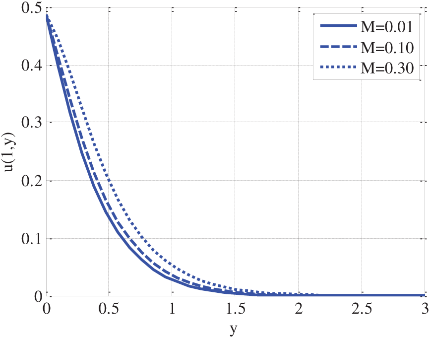
Figure 1: Variation of electromagnetic parameter on velocity profile using
Fig. 2 illustrates the influence of the Eyring–Prandtl fluid parameter
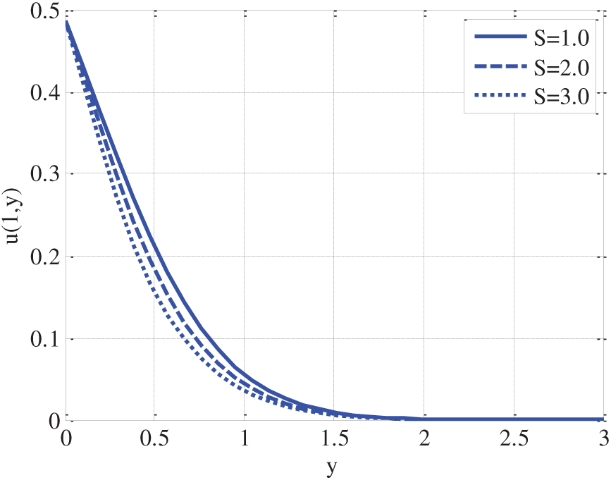
Figure 2: Variation of Eyring parameter on velocity profile using
5.2 Temperature Profile Analysis
Fig. 3 presents the effect of the thermophoresis parameter
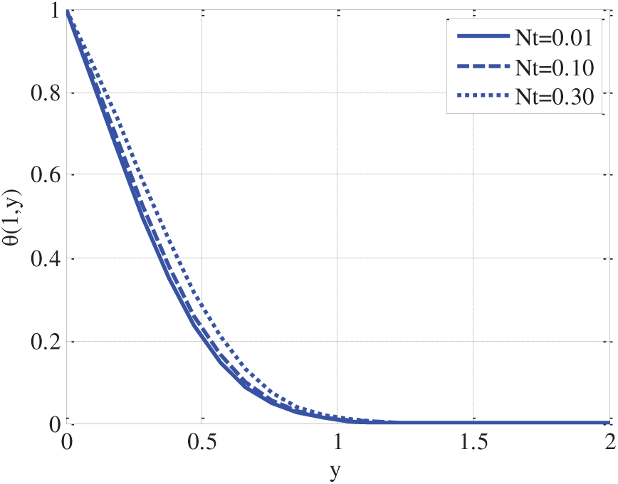
Figure 3: Variation of thermophoresis parameter on temperature profile using
Fig. 4 depicts the influence of the Brownian motion parameter
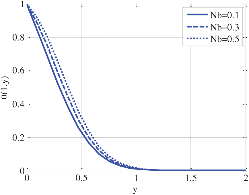
Figure 4: Variation of Brownian motion parameter on temperature profile using
5.3 Concentration Profile Analysis
Fig. 5 illustrates the influence of the Brownian motion parameter
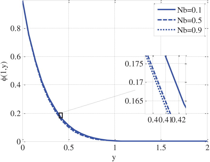
Figure 5: Variation of Brownian motion parameter on nanoparticles concentration profile using
5.4 Different Parameter Analysis
Fig. 6 depicts the effect of the Eyring–Prandtl fluid parameter
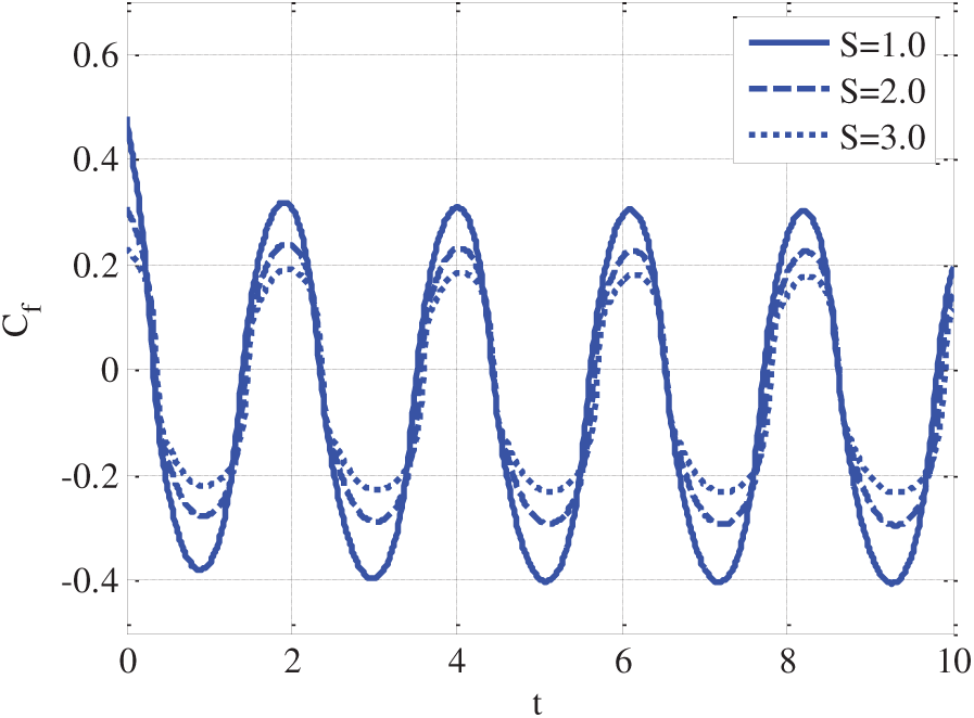
Figure 6: Variation of Eyring parameter on skin friction coefficient using
Fig. 7 illustrates the impact of the Eckert number
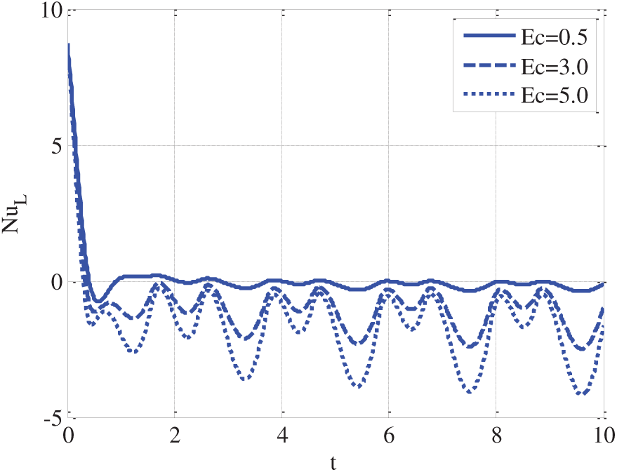
Figure 7: Variation of Eckert number on local Nusselt number using
Fig. 8 demonstrates the effect of the thermophoresis parameter
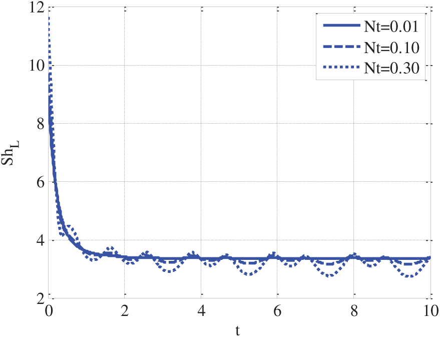
Figure 8: Variation of thermophoresis parameter on local Sherwood number using
The Figs. 9–11 show contour plots of the velocity, temperature, and concentration fields, along with their respective error distributions, at the spatial-time field under the influence of different physical parameters. Fig. 9, left subfigure, depicts the velocity profile that has periodic oscillations and the boundary-layer-like behaviour, which is largely affected by the unsteady forcing term
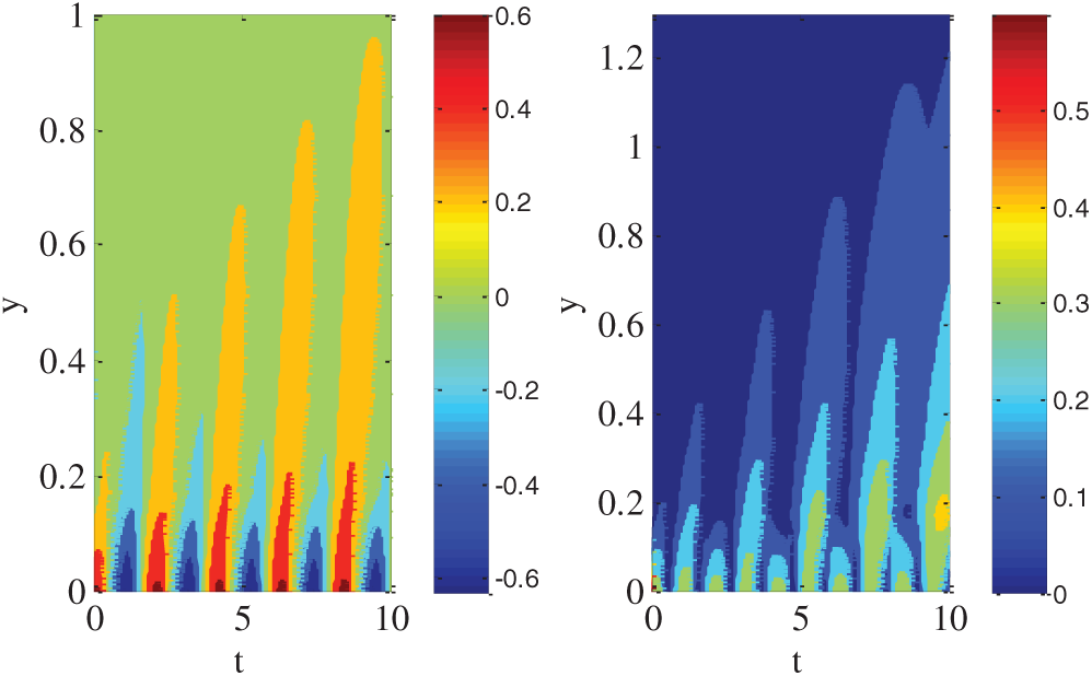
Figure 9: Contour plots for velocity profile and its error from Matlab solver pdepe using
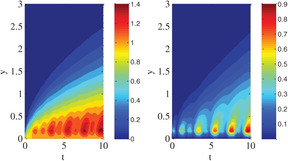
Figure 10: Contour plots for temperature profile and its error from Matlab solver pdepe using
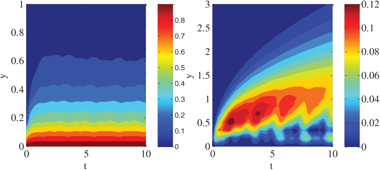
Figure 11: Contour plots for concentration profile and its error from Matlab solver pdepe using
5.6 Computational Time for the Proposed Scheme
Fig. 12 illustrates the variation of computational time associated with the proposed numerical scheme under the influence of fixed physical parameters
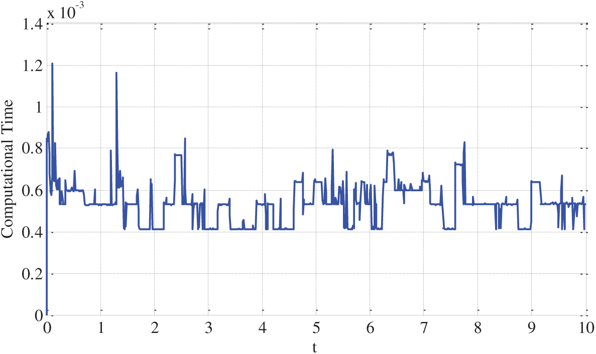
Figure 12: Computational time of the propose scheme using
5.7 Convergence Comparison of Proposed Scheme and Runge-Kutta Method for Stokes First Problem
Fig. 13 illustrates the convergence behavior of two numerical schemes, namely, the proposed scheme and the conventional Runge-Kutta method for solving the classical Stokes first problem under the same spatial and temporal discretization settings, with
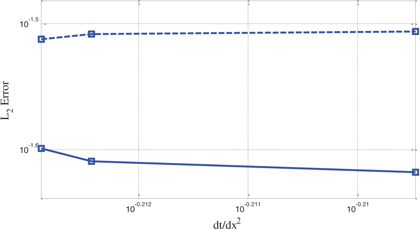
Figure 13: Convergence of two schemes for solving Stokes first problem using
5.8 Validation and Error Analysis Using Stokes’ First Problem
To validate the accuracy and convergence of the proposed three-stage hybrid exponential-Runge-Kutta scheme, we solved the classical Stokes’ first problem, a benchmark test for unsteady viscous flow over a suddenly accelerated plate. This problem has a known exact analytical solution, enabling us to compute numerical errors. The governing equation for Stokes’ first problem is:
The exact solution is:
where
We apply both the proposed scheme and the classical 4th-order Runge–Kutta scheme to this problem and calculate the
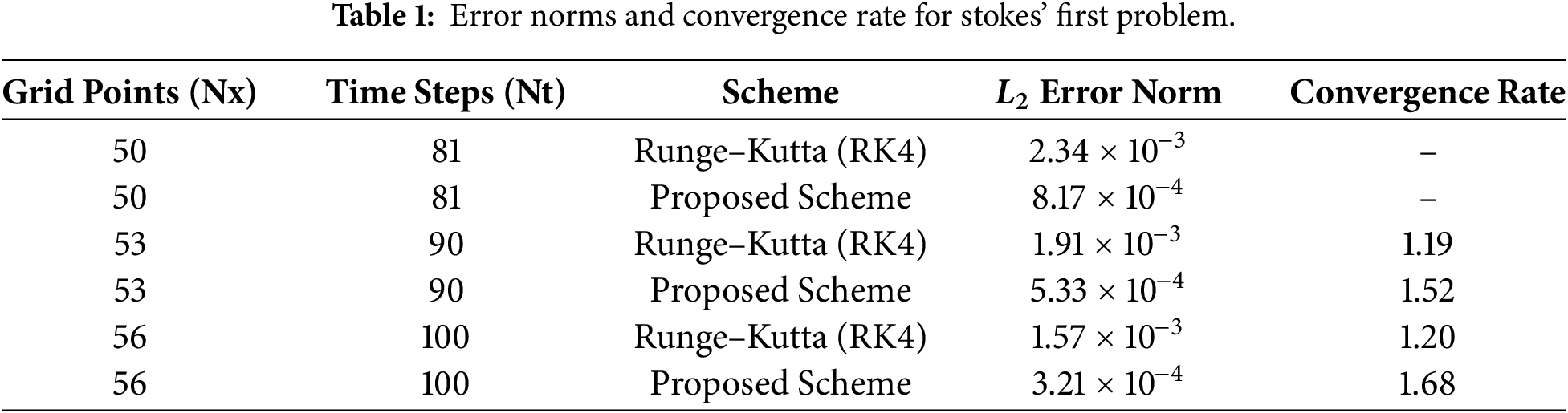
The results confirm that the proposed scheme exhibits significantly lower error norms than the classical RK4 scheme at all tested grid resolutions. Furthermore, the observed convergence rate is closer to 1.5–1.7 for the proposed method, indicating superior accuracy and robustness. This validates the implementation’s correctness and demonstrates the method’s potential to solve time-dependent problems in nanofluid dynamics with greater efficiency and precision.
6 Neural Network-Based Surrogate Model for Predicting Skin Friction Coefficient and Local Sherwood Number
To minimize the computational burden of repeatedly solving the unsteady non-linear PDE governing Eyring–Prandtl nanofluid flow over a Riga plate, a surrogate model based on a feedforward artificial neural network is developed. The target is to predict the skin friction coefficient accurately
6.1 Neural Network Configuration and Training Protocol
The surrogate model architecture and training methodology were designed to achieve high predictive accuracy and generalization capability. The network configuration includes an Input Layer: 5 neurons corresponding to the input parameters
• Training/Validation/Testing Split: The data was split into 70% for training, 15% for validation, and 15% for testing.
• Loss Function: Mean Squared Error (MSE) was minimized during training.
• Regularization: A regularization coefficient
• Cross-validation techniques were employed to monitor generalization ability.
Each simulation case used to generate training data involved solving the system under fixed conditions (e.g.,
• RMSE (Root Mean Square Error) as a statistical metric,
• Regression plots (see Fig. 14) comparing predicted and true values of
• Error histograms and prediction scatter plots.
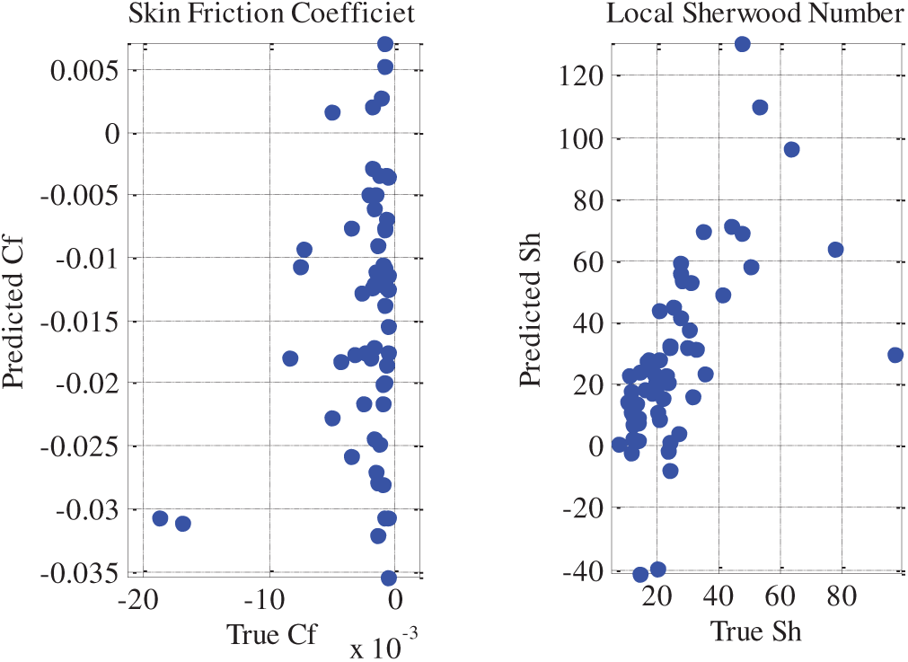
Figure 14: Predicted and True Skin friction coefficient and local Sherwood number using
The RMSE formula is used to evaluate the ANN model’s prediction performance. It is given by:
where
This trained neural network model can now rapidly estimate surface characteristics, such as shear stress and mass transfer rate, for arbitrary combinations of the governing physical parameters, thus enabling efficient sensitivity analysis and real-time design applications in nanofluid dynamics.
Fig. 15 is the schematic illustration of the artificial neural network (ANN) architecture that clearly depicts: Input layer: Consisting of 8 neurons, each corresponding to one of the dimensionless governing parameters (e.g.,
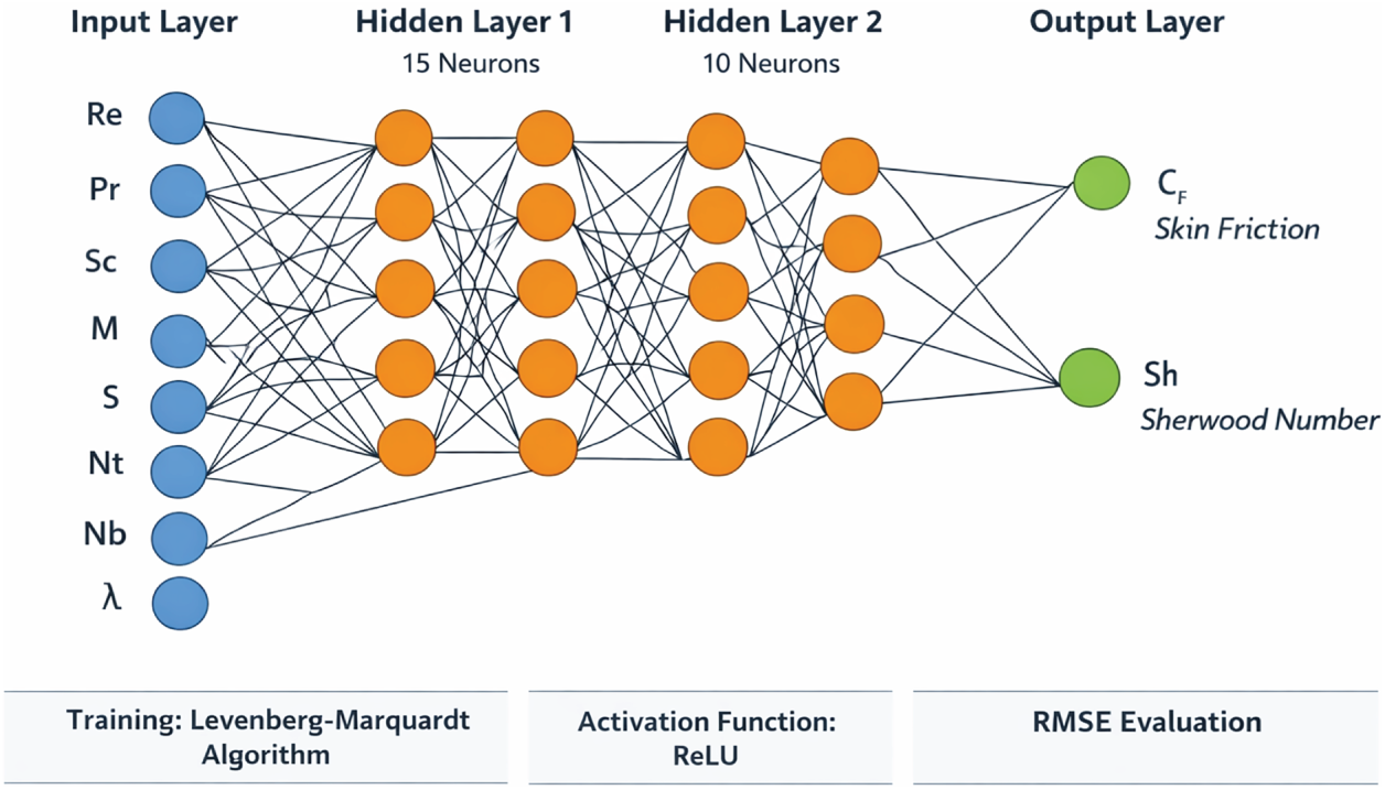
Figure 15: Schematic illustration of the artificial neural network (ANN) for flow prediction.
The selected number of hidden layers and neurons was determined through trial-and-error and performance benchmarking to minimize validation loss while avoiding overfitting. The two-layer configuration provided the best trade-off between model complexity and accuracy. Increasing the number of layers or neurons beyond this did not significantly improve performance but did increase computational cost.
Fig. 14 presents scatter plots comparing the predicted and true values of two key physical quantities: the skin friction coefficient (left) and the local Sherwood number (right), both obtained using a neural network-based surrogate model. The horizontal axes in both subplots represent the true (reference) values obtained from the numerical scheme, while the vertical axes represent the corresponding values predicted by the neural network. Ideally, all points should lie on the 45-degree line (i.e., predicted = true), indicating perfect agreement. In the left plot, corresponding to the skin friction coefficient, most of the data points cluster tightly along the ideal diagonal line, confirming that the neural network accurately captures the non-linear dependence of wall shear stress on the input parameters (such as
The error histogram of the neural network model predicting the skin friction coefficient and the local Sherwood number is shown in Fig. 16. It provides a statistical summary of the model’s accuracy on the training and validation samples. The horizontal axis shows the prediction error (i.e., the difference between predicted and actual values), whereas the vertical axis shows the frequency of these errors. The errors mostly cluster around zero, with the central bars high, indicating that the model’s predictions are close to the actual values and exhibit little deviation. The blue bars correspond to the training data, and the green bars correspond to the validation data, both with symmetric, narrow distributions around the zero-error line (marked in orange). The observation indicates that the neural network has well acquired the underlying mapping and is generalizing well without overfitting, as there are no large spikes or long tails in the error distribution. The histogram therefore supports the argument that the model is strong and sound, and can accurately predict the unknown parameter values within the study’s specified range.
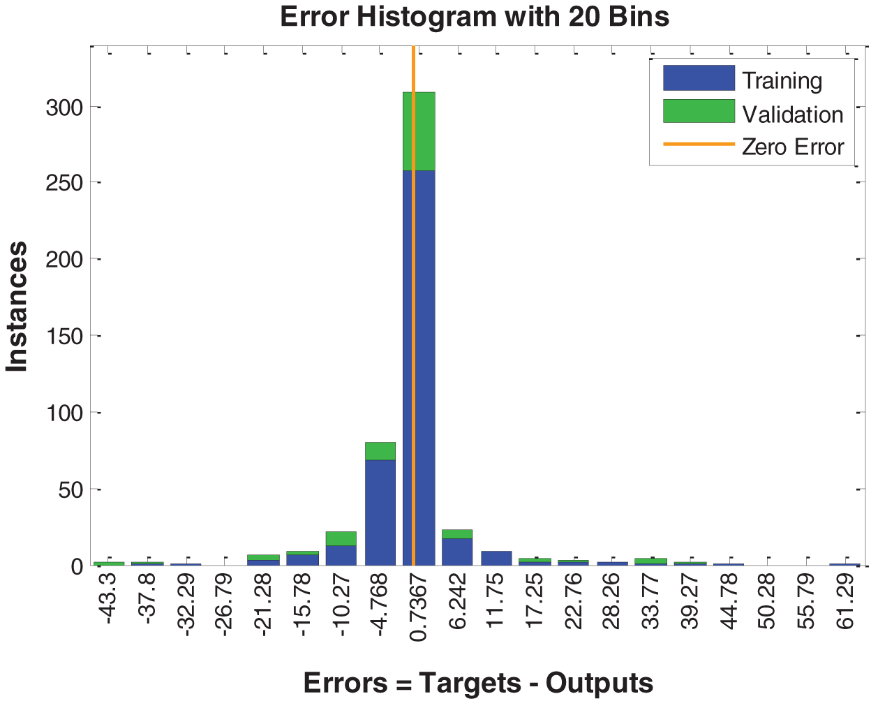
Figure 16: Error histogram for the prediction of skin friction coefficient and local Sherwood number using
Fig. 17 presents regression plots of the neural network’s predictive ability for estimating the skin friction coefficient and the local Sherwood number at the training, validation, and test stages. In both subplots, the horizontal axis shows the actual target values from the numerical simulations, whereas the vertical axis shows the neural network’s estimated target values. The dotted line
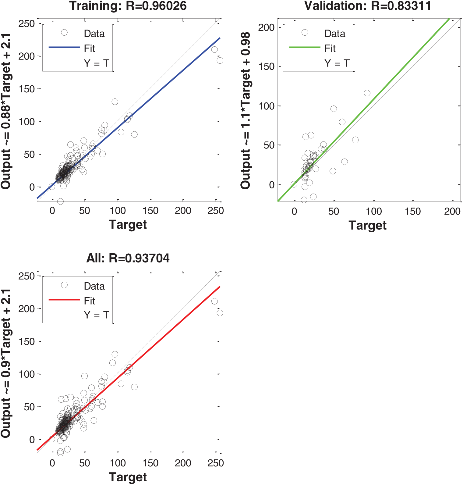
Figure 17: Regression plot of output and target for the prediction of skin friction coefficient and local Sherwood number using
Fig. 18 shows the loss function over 100 training epochs for both the training and validation sets. This figure illustrates how the neural network’s loss converges, providing evidence of model training stability and generalization performance. The rapid convergence and minimal gap between training and validation curves demonstrate the model’s generalization capability and low overfitting risk.
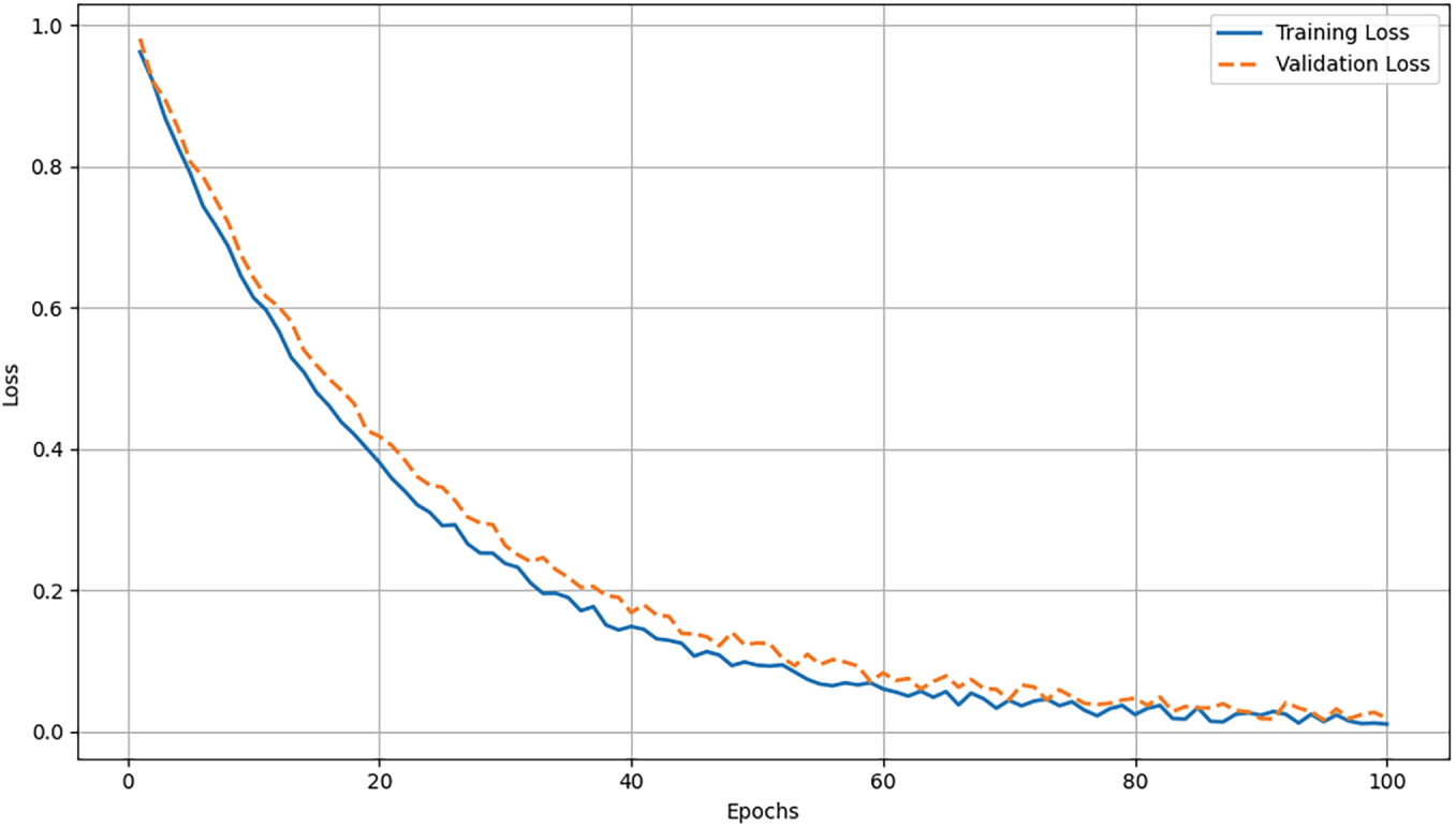
Figure 18: Training and validation loss function plot over 100 epochs for the ANN model predicting skin friction coefficient and local Sherwood number.
6.2 Engineering Implications and Practical Applications
The results presented in this study have significant implications for real-world engineering systems involving nanofluid flow, heat transfer, and electromagnetic actuation. The observed increase in fluid velocity with increasing electromagnetic parameter M highlights the effectiveness of the Riga plate in enhancing flow control, which is directly applicable to MHD-based micro-pumps, lab-on-a-chip devices, and magnetically controlled cooling systems. In such systems, enhanced near-wall flow velocity reduces stagnation zones, promoting efficient heat and mass transfer in microscale domains. The role of the Eyring–Prandtl parameter
This paper presents a three-stage, third-order accurate modified finite-difference approximation for the numerical solution of time-dependent partial differential equations with first-order time derivatives. Spatial discretisation has been performed using a high-order compact scheme to improve accuracy and numerical stability. The strength and soundness of the suggested numerical system have been established by applying it to a pair of reference benchmark problems: the Eyring-Prandtl nanofluid flow over a Riga plate and a linear parabolic test problem with an analytical solution.
Besides the numerical study, it has incorporated an artificial intelligence-based neural network model to predict the skin friction coefficient and the local Sherwood number using governing physical parameters, such as the Reynolds number, Prandtl number, Schmidt number, thermophoresis parameter, and Brownian motion parameter. Numerical targets and neural outputs have been shown to agree strongly, as the neural model’s predictive performance has been verified through regression analysis and error histograms. The concluding points can be expressed as
1. The velocity profile increases with increasing electromagnetic (Riga plate) parameter, confirming the accelerating effect of Lorentz forces on near-wall nanofluid motion.
2. The local Nusselt number decreases with increasing Eckert number, indicating that viscous dissipation dominates over conductive heat transfer.
3. The predicted skin friction coefficient and local Sherwood number are sensitive to the proportion of data used for neural network training and validation, highlighting the importance of dataset optimization in AI-based prediction.
4. The proposed hybrid numerical scheme yields significantly lower numerical error than the classical Runge–Kutta scheme of the same order for comparable step sizes, demonstrating superior accuracy and computational efficiency.
Generally, the current work renders an effective hybrid numerical-artificial intelligence model that can forecast the necessary transports in the electromagnetically actuated non-Newtonian nanofluid flows. The suggested methodology has strong prospects for immediate engineering applications in predictive, optimization, and adaptive control of progressive thermal and mass-transfer apparatus involving Riga plates, nanofluids, and non-Newtonian transport phenomena.
1. Modeling Assumptions: The study assumes a one-dimensional, laminar, incompressible, and homogeneous Eyring–Prandtl nanofluid flow, which may limit the applicability of the results to more complex three-dimensional, turbulent, or compressible flow configurations.
2. Idealized Boundary Conditions: The wall is assumed to move with a constant slip velocity and maintain constant temperature and nanoparticle concentration, which may not fully reflect real-world engineering surfaces with temperature-dependent or spatially varying properties.
3. Neglected Physical Effects: Effects such as nanoparticle aggregation, radiative heat transfer, and Joule heating are not considered in this formulation. These factors can influence heat and mass transfer significantly in high-temperature or electrically conducting applications.
4. Simplified Geometry: The use of a flat Riga plate in Cartesian coordinates excludes curvature or axisymmetric effects that may arise in real devices such as pipes or rotating machinery.
5. Training Dataset Generalizability: The artificial neural network was trained on data generated from specific parameter ranges (e.g.,
The proposed third-order-accurate hybrid time integrator, combining an exponential integrator and Runge–Kutta stages, is novel in its application to Eyring–Prandtl nanofluid flow under electromagnetic (Riga plate) actuation with heat and mass transfer. Unlike classical schemes, our method efficiently handles stiff non-linearities without requiring implicit solvers or linearization, while maintaining high temporal accuracy. The integration of an artificial neural network (ANN) for rapid prediction of the skin friction coefficient and the Sherwood number is a novel contribution. This AI surrogate model provides a computationally inexpensive alternative for real-time parametric studies in engineering design. The results offer actionable insights for thermal management in microfluidic systems, MHD pumps, cooling devices, and coating technologies where control over surface drag and mass transfer is critical. The parametric analysis reveals how electromagnetic forcing, Brownian motion, and thermophoresis can be tuned to optimize flow and thermal characteristics.
Future research may extend the present framework to three-dimensional, turbulent flow regimes, incorporate nanoparticle aggregation, radiative heat transfer, and Joule heating, and explore temperature-dependent thermophysical properties. From a computational perspective, integrating physics-informed neural networks (PINNs) or hybrid deep learning architectures could further enhance predictive capability. Additionally, experimental validation and application of the proposed model to industrial MHD pumps, microchannel heat exchangers, and coating processes represent promising directions for advancing both theoretical and applied research.
Acknowledgement: This research was supported and funded by the Deanship of Scientific Research, Imam Mohammad Ibn Saud Islamic University (IMSIU), Saudi Arabia.
Funding Statement: This work was supported and funded by the Deanship of Scientific Research at Imam Mohammad Ibn Saud Islamic University (IMSIU) (grant number IMSIU-DDRSP2603).
Author Contributions: Conceptualization, methodology, and analysis, Yasir Nawaz; funding acquisition, Nabil Kerdid; investigation, Muhammad Shoaib Arif; methodology, Mairaj Bibi; project administration, Nabil Kerdid; resources, Mairaj Bibi; supervision, Muhammad Shoaib Arif; visualization, Nabil Kerdid; writing—review and editing, Muhammad Shoaib Arif; proofreading and editing, Nabil Kerdid. All authors reviewed and approved the final version of the manuscript.
Availability of Data and Materials: The datasets generated and/or analyzed during the current study are available from the corresponding author on reasonable request.
Ethics Approval: Not applicable.
Conflicts of Interest: The authors declare no conflicts of interest.
References
1. Gailitis A, Lielausis O, Platacis E, Gerbeth G, Stefani F. Riga dynamo experiment and its theoretical background. Phys Plasmas. 2004;11(5):2838–43. doi:10.1063/1.1666361. [Google Scholar] [CrossRef]
2. Choi SUS. Enhancing thermal conductivity of fluids with nanoparticles. In: Proceedings of the 1995 International Mechanical Engineering Congress and Exposition; 1995 Nov 12–17; San Francisco, CA, USA. p. 99–105. doi:10.1115/IMECE1995-0926. [Google Scholar] [CrossRef]
3. Buongiorno J. Convective transport in nanofluids. J Heat Transf. 2006;128(3):240–50. doi:10.1115/1.2150834. [Google Scholar] [CrossRef]
4. Islam S, Khan A, Deebani W, Bonyah E, Alreshidi NA, Shah Z. Influences of Hall current and radiation on MHD micropolar non-Newtonian hybrid nanofluid flow between two surfaces. AIP Adv. 2020;10(5):055015. doi:10.1063/1.5145298. [Google Scholar] [CrossRef]
5. Alempour SM, Abbasian Arani AA, Najafizadeh MM. Numerical investigation of nanofluid flow characteristics and heat transfer inside a twisted tube with elliptic cross section. J Therm Anal Calorim. 2020;140(3):1237–57. doi:10.1007/s10973-020-09337-z. [Google Scholar] [CrossRef]
6. Rasool G, Shafiq A, Khan I, Baleanu D, Nisar KS, Shahzadi G. Entropy generation and consequences of MHD in darcy-forchheimer nanofluid flow bounded by non-linearly stretching surface. Symmetry. 2020;12(4):652. doi:10.3390/sym12040652. [Google Scholar] [CrossRef]
7. Tanveer A, Malik MY. Slip and porosity effects on peristalsis of MHD Ree-Eyring nanofluid in curved geometry. Ain Shams Eng J. 2021;12(1):955–68. doi:10.1016/j.asej.2020.04.008. [Google Scholar] [CrossRef]
8. Khan MI, Kadry S, Chu YM, Khan WA, Kumar A. Exploration of Lorentz force on a paraboloid stretched surface in flow of Ree-Eyring nanomaterial. J Mater Res Technol. 2020;9(5):10265–75. doi:10.1016/j.jmrt.2020.07.017. [Google Scholar] [CrossRef]
9. Nadeem S, Khan MN, Abbas N. Transportation of slip effects on nanomaterial micropolar fluid flow over exponentially stretching. Alex Eng J. 2020;59(5):3443–50. doi:10.1016/j.aej.2020.05.024. [Google Scholar] [CrossRef]
10. Waqas H, Imran M, Khan SU, Shehzad SA, Meraj MA. Slip flow of Maxwell viscoelasticity-based micropolar nanoparticles with porous medium: a numerical study. Appl Math Mech. 2019;40(9):1255–68. doi:10.1007/s10483-019-2518-9. [Google Scholar] [CrossRef]
11. Nadeem S, Abbas N, Malik MY. Heat transport in CNTs based nanomaterial flow of non-Newtonian fluid having electro magnetize plate. Alex Eng J. 2020;59(5):3431–42. doi:10.1016/j.aej.2020.05.022. [Google Scholar] [CrossRef]
12. Hayat T, Yaqoob R, Qayyum S, Alsaedi A. Entropy generation optimization in nanofluid flow by variable thicked sheet. Phys A Stat Mech Appl. 2020;551(19):124022. doi:10.1016/j.physa.2019.124022. [Google Scholar] [CrossRef]
13. Alic F. Entransy dissipation analysis and new irreversibility dimension ratio of nanofluid flow through adaptive heating elements. Energies. 2020;13(1):114. doi:10.3390/en13010114. [Google Scholar] [CrossRef]
14. Mkhatshwa MP, Motsa SS, Ayano MS, Sibanda P. MHD mixed convective nanofluid flow about a vertical slender cylinder using overlapping multi-domain spectral collocation approach. Case Stud Therm Eng. 2020;18:100598. doi:10.1016/j.csite.2020.100598. [Google Scholar] [CrossRef]
15. Tlili I, Shahmir N, Ramzan M, Kadry S, Kim JY, Nam Y, et al. A novel model to analyze Darcy Forchheimer nanofluid flow in a permeable medium with Entropy generation analysis. J Taibah Univ Sci. 2020;14(1):916–30. doi:10.1080/16583655.2020.1790171. [Google Scholar] [CrossRef]
16. Khan I, Ullah K, Chu YM, Nisar K, Al-Khaled K. Oldroyd-B nanofluid-flow between stretching disks with thermal slip and multiple flow features. Therm Sci. 2020;24(Suppl 1):83–94. doi:10.2298/tsci20s1083k. [Google Scholar] [CrossRef]
17. Shaw S, Dogonchi AS, Nayak MK, Makinde OD. Impact of entropy generation and nonlinear thermal radiation on darcy-forchheimer flow of MnFe2O4-casson/water nanofluid due to a rotating disk: application to brain dynamics. Arab J Sci Eng. 2020;45(7):5471–90. doi:10.1007/s13369-020-04453-2. [Google Scholar] [CrossRef]
18. Hayat T, Haider F, Muhammad T, Alsaedi A. On Darcy-Forchheimer flow of carbon nanotubes due to a rotating disk. Int J Heat Mass Transf. 2017;112:248–54. doi:10.1016/j.ijheatmasstransfer.2017.04.123. [Google Scholar] [CrossRef]
19. Muskat M. The flow of homogeneous fluids through porous media. Soil Sci. 1938;46(2):169. doi:10.1097/00010694-193808000-00008. [Google Scholar] [CrossRef]
20. Seddeek MA. Influence of viscous dissipation and thermophoresis on Darcy-Forchheimer mixed convection in a fluid saturated porous media. J Colloid Interface Sci. 2006;293(1):137–42. doi:10.1016/j.jcis.2005.06.039. [Google Scholar] [PubMed] [CrossRef]
21. Francis P, Sambath P, Noeiaghdam S, Fernandez-Gamiz U, Dinarvand S. Computational analysis of bioconvective MHD hybrid nanofluid flow of non-Newtonian fluid over cone/plate:a study based on the Cattaneo-Christov heat and mass flux model. Eng Sci Technol Int J. 2025;63:101970. doi:10.1016/j.jestch.2025.101970. [Google Scholar] [CrossRef]
22. Arulmozhi S, Sukkiramathi K, Santra SS, Edwan R, Fernandez-Gamiz U, Noeiaghdam S. Heat and mass transfer analysis of radiative and chemical reactive effects on MHD nanofluid over an infinite moving vertical plate. Results Eng. 2022;14(1):100394. doi:10.1016/j.rineng.2022.100394. [Google Scholar] [CrossRef]
23. Hayat T, Muhammad T, Al-Mezal S, Liao SJ. Darcy-Forchheimer flow with variable thermal conductivity and Cattaneo-Christov heat flux. Int J Numer Methods Heat Fluid Flow. 2016;26(8):2355–69. doi:10.1108/hff-08-2015-0333. [Google Scholar] [CrossRef]
24. Mohana CM, Kumar BR. Shape effects of Darcy-Forchheimer unsteady three-dimensional CdTe-C/H2O hybrid nanofluid flow over a stretching sheet with convective heat transfer. Phys Fluids. 2023;35(9):092002. doi:10.1063/5.0168503. [Google Scholar] [CrossRef]
25. Animasaun IL, Kumar TK, Noah FA, Okoya SS, Al-Mdallal QM, Bhatti MM. Insight into Darcy flow of ternary-hybrid nanofluid on horizontal surfaces: exploration of the effects of convective and unsteady acceleration. J Appl Math Mech. 2023;103(5):e202200197. doi:10.1002/zamm.202200197. [Google Scholar] [CrossRef]
26. Prakash J, Tripathi D, Bég OA. Computation of EMHD ternary hybrid non-Newtonian nanofluid over a wedge embedded in a Darcy-Forchheimer porous medium with Zeta potential and wall suction/injection effects. Int J Ambient Energy. 2023;44(1):2155–69. doi:10.1080/01430750.2023.2224339. [Google Scholar] [CrossRef]
27. Das S, Barman B, Jana RN, Makinde OD. Hall and ion slip currents’ impact on electromagnetic blood flow conveying hybrid nanoparticles through an endoscope with peristaltic waves. BioNanoScience. 2021;11(3):770–92. doi:10.1007/s12668-021-00873-y. [Google Scholar] [CrossRef]
28. Sahoo A, Nandkeolyar R. Entropy generation and dissipative heat transfer analysis of mixed convective hydromagnetic flow of a Casson nanofluid with thermal radiation and Hall current. Sci Rep. 2021;11(1):3926. doi:10.1038/s41598-021-83124-0. [Google Scholar] [PubMed] [CrossRef]
29. Shaheen N, Ramzan M, Alaoui MK. Impact of Hall current on a 3D Casson nanofluid flow past a rotating deformable disk with variable characteristics. Arab J Sci Eng. 2021;46(12):12653–66. doi:10.1007/s13369-021-06060-1. [Google Scholar] [CrossRef]
30. Rashidi S, Esfahani JA, Maskaniyan M. Applications of magnetohydrodynamics in biological systems—a review on the numerical studies. J Magn Magn Mater. 2017;439(1):358–72. doi:10.1016/j.jmmm.2017.05.014. [Google Scholar] [CrossRef]
31. Basavarajappa M, Bhatta D. Lie group analysis of flow and heat transfer of a nanofluid in cone-disk systems with Hall current and radiative heat flux. Math Methods Appl Sci. 2023;46(14):15838–67. doi:10.1002/mma.9429. [Google Scholar] [CrossRef]
32. Zhang L, Zhang H. Numerical simulation of heat and mass transfer in non-Newtonian Casson nanofluids driven nonlinearly by a wedge-shaped stretching plate. Chin J Phys. 2025;95:939–61. doi:10.1016/j.cjph.2025.04.015. [Google Scholar] [CrossRef]
33. Zhang L, Zhang H, Wang S, Song J, Yao X, Wang W. Boundary layer and entropy analysis of non-Newtonian Casson nanofluids moving nonlinearly in a wedge-shaped stretching plate under an unsteady flow. Case Stud Therm Eng. 2024;56(1):104193. doi:10.1016/j.csite.2024.104193. [Google Scholar] [CrossRef]
34. Khan A, Shah RA, Alam MK, Ahmed H, Shahzad M, Rehman S, et al. Computational investigation of an unsteady non-Newtonian and non-isothermal fluid between coaxial contracting channels: a PCM approach. Results Phys. 2021;28:104570. doi:10.1016/j.rinp.2021.104570. [Google Scholar] [CrossRef]
35. Abbas SZ, Khan WA, Waqas M, Irfan M, Asghar Z. Exploring the features for flow of Oldroyd-B liquid film subjected to rotating disk with homogeneous/heterogeneous processes. Comput Methods Programs Biomed. 2020;189:105323. doi:10.1016/j.cmpb.2020.105323. [Google Scholar] [PubMed] [CrossRef]
36. Sangeetha E, De P. Stagnation point flow of bioconvective MHD nanofluids over Darcy-Forchheimer porous medium with thermal radiation and buoyancy effect. BioNanoScience. 2023;13(3):1022–35. doi:10.1007/s12668-023-01132-y. [Google Scholar] [CrossRef]
37. Gomathi N, Poulomi D. Entropy optimization on EMHD Casson Williamson penta-hybrid nanofluid over porous exponentially vertical cone. Alex Eng J. 2024;108:590–610. doi:10.1016/j.aej.2024.07.092. [Google Scholar] [CrossRef]
38. Shafiq A, Çolak AB, Sindhu TN. Significance of EMHD graphene oxide (GO) water ethylene glycol nanofluid flow in a Darcy-Forchheimer medium by machine learning algorithm. Eur Phys J Plus. 2023;138(3):213. doi:10.1140/epjp/s13360-023-03798-5. [Google Scholar] [CrossRef]
39. Zhao TH, Khan MI, Chu YM. Artificial neural networking (ANN) analysis for heat and entropy generation in flow of non-Newtonian fluid between two rotating disks. Math Methods Appl Sci. 2023;46(3):3012–30. doi:10.1002/mma.7310. [Google Scholar] [CrossRef]
40. Sharma BK, Sharma P, Mishra NK, Fernandez-Gamiz U. Darcy-Forchheimer hybrid nanofluid flow over the rotating Riga disk in the presence of chemical reaction: artificial neural network approach. Alex Eng J. 2023;76(1):101–30. doi:10.1016/j.aej.2023.06.014. [Google Scholar] [CrossRef]
41. Boumari E, Amiri MM, Khadang A, Maddah H, Ahmadi MH, Sharifpur M. Numerical investigation of heat transfer in helical tubes modified with aluminum oxide nanofluid and modeling of data obtained by artificial neural network. Numer Heat Transf Part A Appl. 2023;83(3):265–84. doi:10.1080/10407782.2022.2091367. [Google Scholar] [CrossRef]
42. Sundar LS, Mewada HK. Experimental entropy generation, exergy efficiency and thermal performance factor of CoFe2O4/water nanofluids in a tube predicted with ANFIS and MLP models. Int J Therm Sci. 2023;190:108328. doi:10.1016/j.ijthermalsci.2023.108328. [Google Scholar] [CrossRef]
43. Ouri H, Selimefendigil F, Bouterra M, Omri M, Alshammari BM, Kolsi L. MHD hybrid nanofluid convection and phase change process in an L-shaped vented cavity equipped with an inner rotating cylinder and PCM-packed bed system. Alex Eng J. 2023;63:563–82. doi:10.1016/j.aej.2022.08.016. [Google Scholar] [CrossRef]
44. Beiki H. Developing convective mass transfer of nanofluids in fully developed flow regimes in a circular tube: modeling using fuzzy inference system and ANFIS. Int J Heat Mass Transf. 2021;173:121285. doi:10.1016/j.ijheatmasstransfer.2021.121285. [Google Scholar] [CrossRef]
45. Ahmadi MH, Ghazvini M, Maddah H, Kahani M, Pourfarhang S, Pourfarhang A, et al. Prediction of the pressure drop for CuO/(ethylene glycol-water) nanofluid flows in the car radiator by means of artificial neural networks analysis integrated with genetic algorithm. Phys A Stat Mech Appl. 2020;546:124008. doi:10.1016/j.physa.2019.124008. [Google Scholar] [CrossRef]
46. Hojjat M. Nanofluids as coolant in a shell and tube heat exchanger: ANN modeling and multi-objective optimization. Appl Math Comput. 2020;365:124710. doi:10.1016/j.amc.2019.124710. [Google Scholar] [CrossRef]
47. Shafiq A, Çolak AB, Sindhu TN. Optimization of the numerical treatment of the Darcy-Forchheimer flow of Ree-Eyring fluid with chemical reaction by using artificial neural networks. Int J Numer Methods Fluids. 2023;95(1):176–92. doi:10.1002/fld.5147. [Google Scholar] [CrossRef]
48. Çolak AB, Sindhu TN, Ahmad Lone S, Shafiq A, Abushal TA. Reliability study of generalized Rayleigh distribution based on inverse power law using artificial neural network with Bayesian regularization. Tribol Int. 2023;185:108544. doi:10.1016/j.triboint.2023.108544. [Google Scholar] [CrossRef]
49. Kamsuwan C, Wang X, Seng LP, Xian CK, Piemjaiswang R, Piumsomboon P, et al. Simulation of nanofluid micro-channel heat exchanger using computational fluid dynamics integrated with artificial neural network. Energy Rep. 2023;9:239–47. doi:10.1016/j.egyr.2022.10.412. [Google Scholar] [CrossRef]
50. Habib S, Nasir S, Khan Z, Berrouk AS, Islam S, Aamir A. Machine-assisted simulation of heat and mass transfer through a porous Riga surface with chemical reactions and radiation effects. J Therm Anal Calorim. 2025;150(10):7949–70. doi:10.1007/s10973-025-14191-y. [Google Scholar] [CrossRef]
51. Nasir S, Berrouk AS, Gul T. Analysis of chemical reactive nanofluid flow on stretching surface using numerical soft computing approach for thermal enhancement. Eng Appl Comput Fluid Mech. 2024;18(1):2340609. doi:10.1080/19942060.2024.2340609. [Google Scholar] [CrossRef]
Cite This Article
 Copyright © 2026 The Author(s). Published by Tech Science Press.
This work is licensed under a Creative Commons Attribution 4.0 International License , which permits unrestricted use, distribution, and reproduction in any medium, provided the original work is properly cited.
 Downloads
 Citation Tools