Spectral-Integrated Neural Networks for Transient Heat Conduction in Thin-Walled Structures

1  Introduction

Thin-walled structures are widely used in modern engineering systems due to their advantages in material efficiency, lightweight design, and functional integration. Typical applications include thin films and coatings in electronic devices, protective layers in mechanical components, and embedded sensing elements in smart materials. Despite their practical importance, numerical simulation of thin-walled structures remains challenging because of the severe geometric slenderness and the strong coupling between spatial resolution and numerical stability.

Conventional numerical methods, such as the finite element method (FEM), are frequently employed for heat conduction analysis owing to their generality and mature theoretical foundation [1–5]. However, when applied to thin-walled configurations, FEM often requires extremely refined meshes across the thickness direction to maintain accuracy and stability [5–8]. This leads to ill-conditioned system matrices [9–12], high computational cost, and, in some cases, convergence difficulties. The boundary element method (BEM) offers an alternative by reducing the problem dimensionality and efficiently handling unbounded domains [13–16]. Nevertheless, BEM formulations rely on the availability of fundamental solutions, which limits their applicability to a restricted class of governing equations and material models. Consequently, there is a growing need for alternative numerical approaches capable of efficiently and accurately handling such challenging problems with thin-shapes [17,18].

To overcome these limitations, meshless and data-driven approaches have attracted increasing attention in recent years [19–22]. Among them, physics-informed neural networks (PINNs) provide a flexible framework by embedding governing partial differential equations directly into the training process of neural networks [23–26]. By enforcing physical constraints through loss functions, PINNs are capable of approximating solutions to forward and inverse problems without relying on structured meshes. This paradigm has been successfully explored in a wide range of applications, including solid mechanics, fluid dynamics, heat transfer, and multiphysics systems [27–31]. Complementing these physics-informed approaches, recent studies have also highlighted the effectiveness of ensemble learning techniques. For example, bagging regression has been successfully applied to conduct a comparative analysis of magnetohydrodynamic mixed convective flow of hybrid nanofluids, incorporating radiative heat transfer [32]. Several variants of PINNs have been developed to broaden their applicability, such as conservative PINNs, fractional PINNs, Bayesian PINNs, and variational PINNs [33–36]. Furthermore, the potential of PINNs in thermal analysis has been exemplified by recent studies, such as the prediction of steady-state temperature distributions in convective wavy fins using novel training strategies [37]. For transient problems, PINNs typically rely on automatic differentiation to compute time derivatives, which can lead to high computational cost and deteriorating accuracy, especially for long-time simulations or stiff systems [38].

To address the above challenges, spectral-integrated neural networks (SINNs) were recently introduced as an extension of the PINN framework [39,40]. The key idea of SINNs is to replace direct time differentiation with a spectral integration strategy based on orthogonal polynomial expansions [41]. Spectral integration techniques are well known for their excellent stability and high-order accuracy in temporal discretization, particularly when large time steps are employed. By combining spectral integration with neural network approximation, SINNs enable efficient dynamic analysis without the need for dense temporal sampling [42]. Motivated by these advantages, the present study extends the SINN framework to transient heat conduction problems in thin-walled structures. Such problems are especially challenging due to extreme aspect ratios, where conventional numerical solvers often experience stability issues or prohibitive computational cost.

The remainder of this paper is organized as follows. Section 2 introduces the governing equations of transient heat conduction and presents the spectral-integrated neural network formulation. Section 3 provides a series of numerical examples, including both regular and irregular thin-walled geometries, to assess the accuracy, efficiency, and stability of the proposed method. Finally, Section 4 summarizes the main findings and discusses potential extensions of the present work.

2  Methodology

This section presents the theoretical formulation of the proposed spectral-integrated neural network framework for transient heat conduction analysis. To illustrate the framework, the following 2D transient heat conduction problem is considered [43,44]:

ρcut(x,t)−∇[k∇u(x,t)]=f(x,t),x∈Ω,t∈[0,T].(1)

Assuming Ω is a 2D domain bounded by a surface ∂Ω=Γ, where Γ=ΓD∪ΓN. The system is subject to a prescribed initial condition, together with Dirichlet and Neumann boundary conditions:

u(x,0)=u0(x),x∈Ω,(2)

u(x,t)=u¯(x,t),x∈ΓD,t∈[0,T],(3)

q(x,t)=−k(⋅)∂u(x,t)∂n=q¯(x,t),x∈ΓN,t∈[0,T],(4)

where ρ, c and k denote the mass density, the specific heat and the thermal conductivity, respectively, Ref. [45] is the unknown temperature field, and f(x,t) represents the heat source term.

2.1 Spectral Integration Method

To enhance numerical stability in the temporal domain, this study introduces a new variable U(x,t)=ut(x,t) in Eq. (1), through which the transient heat conduction equation is reformulated as:

ρcU(x,t)−∇[k∇u(x,t)]=f(x,t),x∈Ω,t∈[0,T],(5)

where

u(x,t)=u0+∫0tU(x,τ)dτ.(6)

Within the temporal discretization, this study divides the time interval into multiple subintervals, denoted as [0,T]=[T0=0,T1]∪[T1,T2]∪…∪[Tn−1,Tn=T], with the step size defined as ΔTi=Ti−Ti−1. This study describes the procedure for solving Eq. (5) within the subinterval [T0=0,T1], which can be mapped onto the standard interval [−1,1] by means of a linear transformation. This study employs p Gaussian-type nodes t={tj|j=1,2,⋯,p} within each subinterval and denotes the corresponding values of the new variable at these nodes by U(x)=[U(x,t1),U(x,t2),…,U(x,tp)]. The value of U(x) can be stably and accurately approximated by constructing a Legendre polynomial expansion Lp(U(x),t), whose coefficients are determined through Gaussian quadrature rules [46]. Through the integration of Lp(U(x),t) over the time span [T0=0,T1], a linear mapping ΔTiS is established that links U(x) with its temporal integral, expressed as

ΔTSU(x)=[∫t0t1Lp(U(x),τ)dτ,∫t0t2Lp(U(x),τ)dτ,…,∫t0tmLp(U(x),τ)dτ]T,(7)

where in S is a spectral integration matrix independent of time step ΔTi. A detailed discussion of this matrix is provided in Refs. [46,47]. Using the spectral integral matrix, Eq. (6) can be discretized as:

u(x)=u0(x)+ΔTSU(x),(8)

where u(x)=[u(x,t1),u(x,t2),⋯,u(x,tp)]T, u0(x)=[u0(x),u0(x),⋯,u0(x)]T. When Eq. (8) is substituted into the governing equation Eq. (5), the resulting formulation can be explicitly expressed as follows:

ρcU(x)−∇k∇[u0(x)+ΔTSU(x)]=f(x),x∈Ω,(9)

and the corresponding boundary conditions given in Eqs. (3) and (4) can be expressed as follows:

u¯(x)=u0(x)+ΔTSU(x),x∈ΓD,(10)

q¯(x)=−k(⋅)∂(u0(x)+ΔTSU(x))∂n,x∈ΓN,(11)

where f(x) represents [f(x,t1),f(x,t2),⋯,f(x,tp)]T. The system originally governed by Eqs. (1)–(4) in terms of the variable u can equivalently be restated as the new set of Eqs. (9)–(11), expressed in terms of the first-order derivatives U of temperature.

2.2 Spectral-Integrated Neural Networks for Heat Conduction Problem

This study takes the transient heat conduction problem as an example to describe the process and framework of the SINNs. Fig. 1 provides a schematic of the fully connected neural network used to approximate the first-order temporal derivatives U(x,t) of temperature. The network takes (x,t), as input and produces the trial solution U(x,t) at the output layer. Comprising m hidden layers with Nk,(k=1,2,3…,m) neurons in each layer, the network represents the trial solutions as:

U~(x,t,W)=ψ(ηm(ηm−1(…(η1(x^))))),(12)

where ψ corresponds to the linear mapping, which is defined as

ψ(γ)=w^γ+b^,(13)

and ηk(k=1,2,…,m) corresponds to the nonlinear mapping, given by

ηk(γ)=σ(wkγ+bk),k=1,2,…,m.(14)

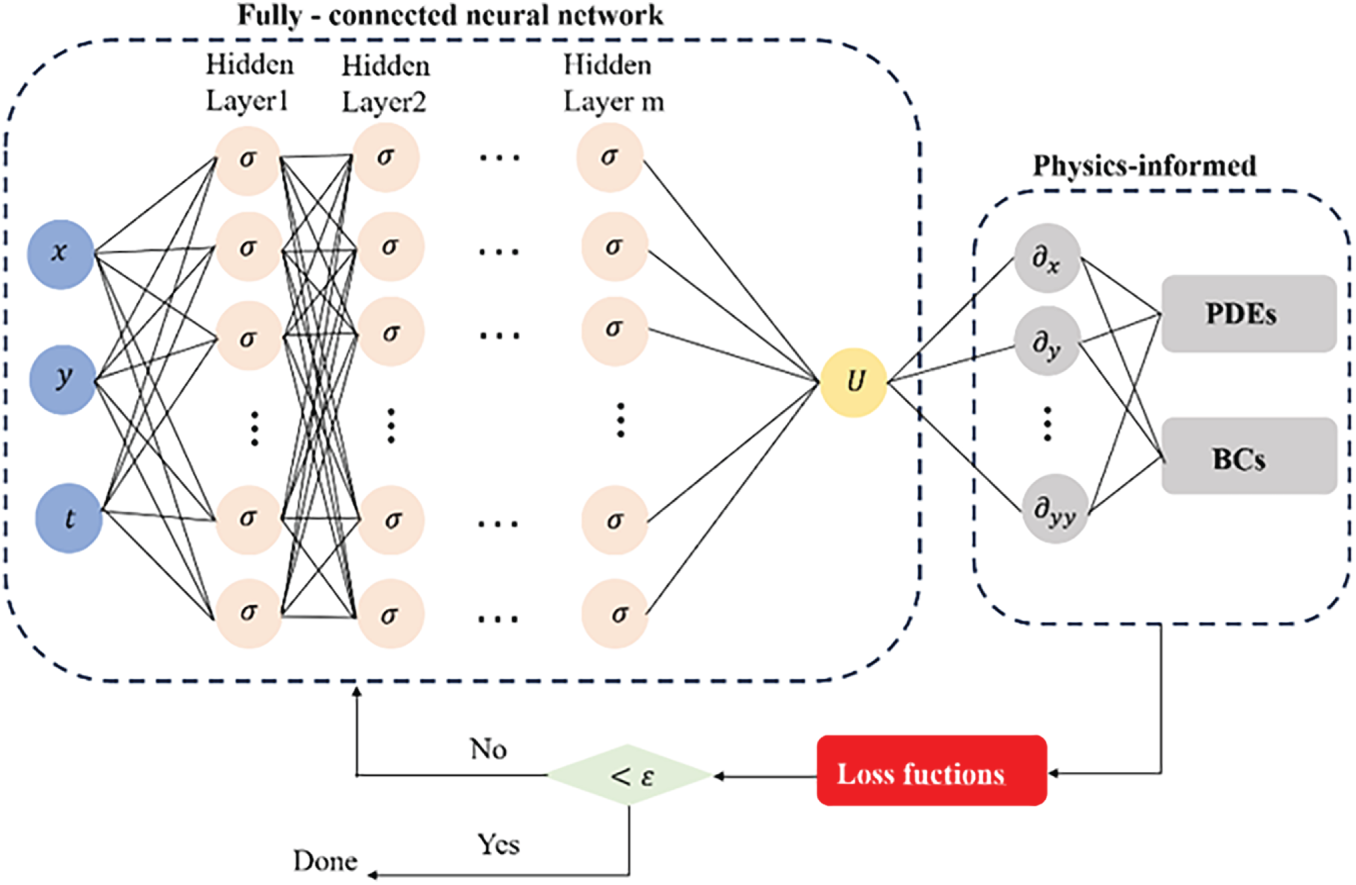
Figure 1: Schematic diagram of the spectral integrated neural networks (SINNs).

In Eqs. (12)–(14), σ denotes the activation function, wk,w^∈Rnm represent the weights, b^,b∈Rnm are biases, and W are vectors of all network parameters, defined as:

W=({wj}j=1m,w^,{bj}j=1m,b^).(15)

This study defines the residuals of the PDE as:

ℓPDE(x;W)=ρ(⋅)c(⋅)U(x;W)−∇k(⋅)∇[u0(x)+ΔTSU(x;W)]−f(x).(16)

In this approach, the governing PDE and the associated boundary conditions are used to constrain the trial solution during the training processes. A corresponding loss function is then introduced, which is minimized to optimize the parameters, as expressed below:

Loss(W)=∑j=1pLossPDE(W)+∑j=1pLossDBC(W)+∑j=1pLossNBC(W),(17)

in which LossPDE, LossDBC and LossNBC are the losses of governing PDE, Dirichlet and Neumann boundary conditions, respectively. NPDE, NNBC and NDBC represent the number of nodes associated with the respective terms. The individual loss components are detailed as follows:

LPDE(W)=1pNPDE∑i=1pNPDE|ℓPDE(xPDE;W)|2,(18)

LDBC(W)=1pNDBC∑i=1pNDBC|u(xDBC,t;W)−u¯(xDBC,t)|2,(19)

LNBC(W)=1pNDBC∑k=1pNDBC|k(⋅)∂u(xNBC,t;W)∂n+q¯(xNBC,t)|2.(20)

Gradient descent is employed to train the parameters W in the fully connected network, using backpropagation to propagate gradients from the loss function. The training process is terminated when the loss falls below a predefined threshold or when the maximum number of iterations is reached.

3  Numerical Experiments

To evaluate the performance of the SINNs in thin-walled structural problems, a series of numerical experiments are conducted on transient heat conduction cases encompassing both non-thin and thin geometries. These experiments are designed to assess the accuracy and effectiveness of the proposed method across a variety of geometric configurations. The numerical accuracy is quantified using the relative error and max absolute error, defined as follows:

Relativeerror=‖u(xl,tl)−u~(xl,tl)‖2‖u(xl,tl)‖2,(21)

L∞=maxl|u(xl,tl)−u~(xl,tl)|,(22)

where (xl,tl) denotes the l-th test node, while u(xl,tl) and u~(xl,tl) respectively stand for the exact (or fabricated) and numerical solutions.

This paper presents four numerical examples for testing. All computational tasks were performed in MATLAB R2023a under the Windows 11 (64-bit) operating system. The computing device is equipped with an Intel Core Ultra 7 155H CPU with a base frequency of 1.40 GHz and 32 GB of memory. In this study, the “fmincon” function provided by MATLAB was used to train the network, which is designed to find the minimum of constrained nonlinear multivariable functions. The main training process was set to a maximum of 5000 iterations.

3.1 Structure without Thin-Shapes

The initial investigation is conducted to assess the capability of SINNs in solving transient heat conduction problem, as illustrated in Fig. 2. For clarity, the governing equation is expressed as follows:

ut(x,t)−∇u(x,t)=f(x,t),x∈Ω,t∈[0s,Ts].(23)

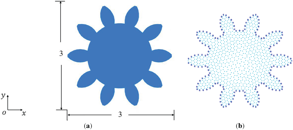
Figure 2: (a) Geometry of gear structure; (b) The distribution of collocation points.

The analytical solution corresponding to this numerical example is:

u(x,t)=cos⁡(t)sin⁡(x+y).(24)

A total of 1150 collocation points are employed, comprising 160 points on the boundary and 990 points within the interior domain. All boundary conditions are prescribed as Dirichlet type. In addition, a time step of Δt=1s is adopted to ensure temporal stability, and 5 Gaussian nodes are used within each time step. Different neural network architectures are often required to effectively handle problems with varying complexity and geometric characteristics. In this example, the performance of the proposed SINNs is systematically assessed by varying both the number of hidden layers and the number of neurons per layer. This architectural tuning aims to identify an optimal network configuration that balances accuracy, computational efficiency, and training stability for the given problem. The corresponding relative errors are summarized in Table 1. The results indicate that increasing the number of hidden layers has only a marginal influence on solution accuracy in transient heat conduction problems. And as demonstrated by the research findings, the results obtained from the [20, 20] architecture and those from the three-hidden-layer network are of the same order of magnitude. To enhance the efficiency of the study, this study will adopt the same [20, 20] network architecture in the subsequent numerical examples.

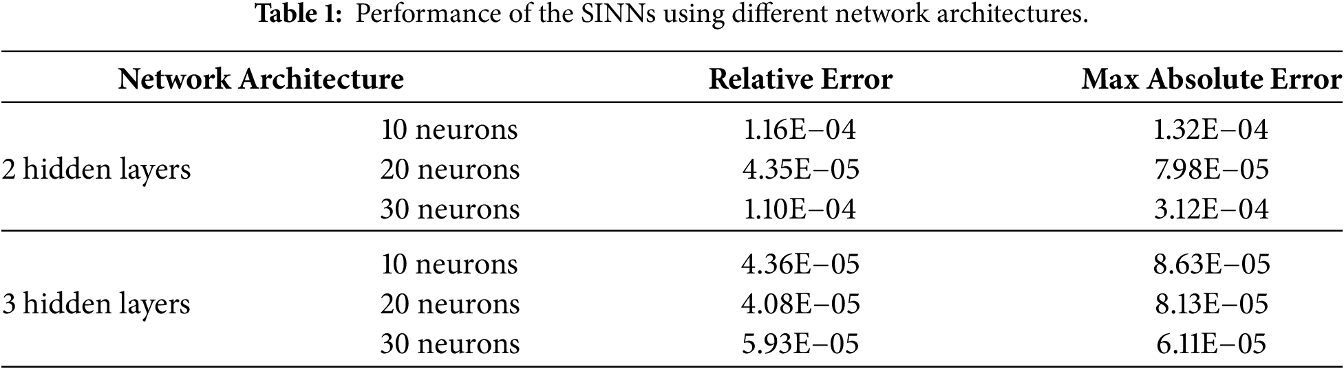
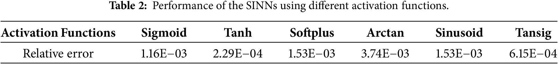
For a more comprehensive evaluation of the proposed method, the network architecture is configured with two fully connected hidden layers, each consisting of 20 neurons, while different activation functions are employed during training. As presented in Table 2, the SINNs consistently achieve high accuracy, with relative errors ranging from 2×10−4 and 4×10−3, thereby demonstrating the robustness of the method with respect to the choice of activation function. Table 3 presents the runtime and the number of iterations required for PINNs and SINNs to reduce the loss function value to 10−6. As we can see, the SINNs achieve superior computational efficiency compared to the PINNs.

As illustrated in Fig. 3, the relative temperature errors at 1 s, 3 s, and 5 s are evaluated using the Sinusoid function. The results demonstrate that, even with a relatively large time step of 1 s, the proposed numerical scheme maintains a high level of accuracy throughout the simulation period, underscoring its robustness and reliability. Moreover, in the comprehensive evaluation involving a complex domain, the findings further confirm the capability of the SINNs to deliver accurate solutions for 2D non-thin-body heat transfer problems.

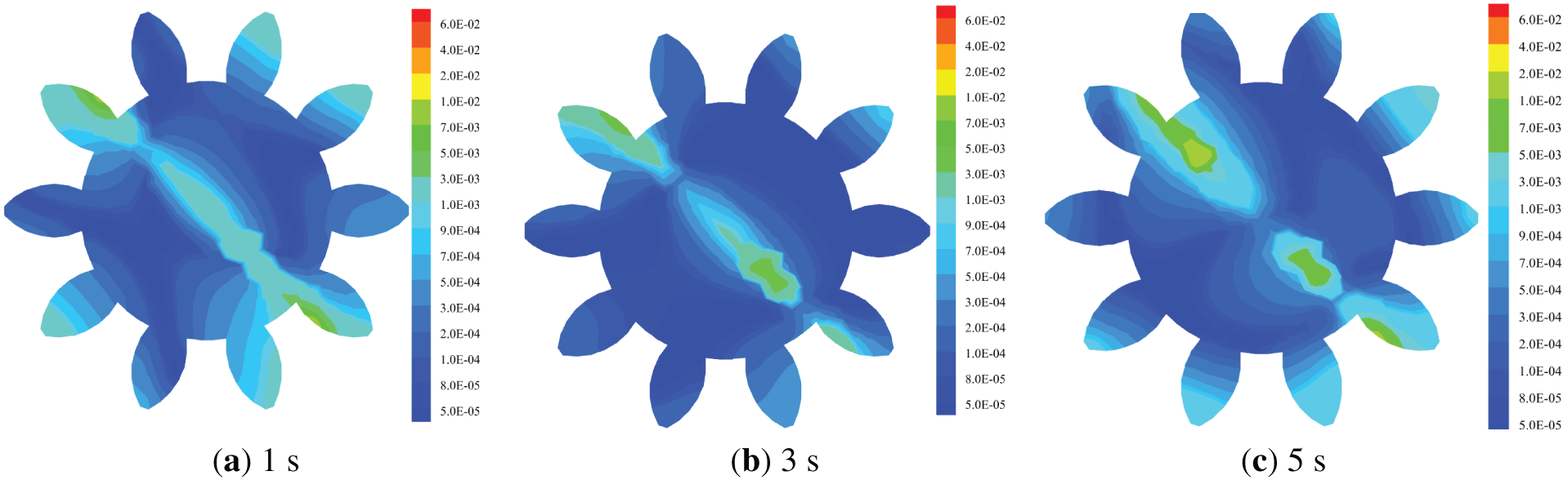
Figure 3: Relative errors of temperature at t=1,3,5s of this model.

3.2 Transient Heat Conduction in a Rectangular Thin-Body Structure

As the second numerical example, this study investigates transient heat conduction in a thin rectangular structure, as illustrated in Fig. 4. The governing equation can be expressed as follows:

ρ(⋅)c(⋅)ut(x,t)−∇[k(⋅)∇u(x,t)]=f(x,t),x∈Ω,t∈[0s,Ts],(25)

where the material parameters ρ(x)c(x)=x+y, k(x)=x2+y2. The analytical temperature solution is given as follows:

u(x,t)=cos⁡(t)[cos⁡(x)cosh⁡(y)+sin⁡(x)sinh⁡(y)],(26)

where the source term f(x,t) can be derived using Eq. (26).

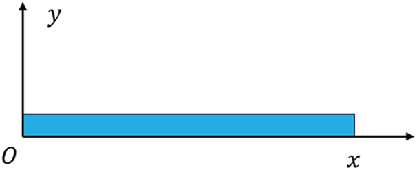
Figure 4: A thin rectangular domain.

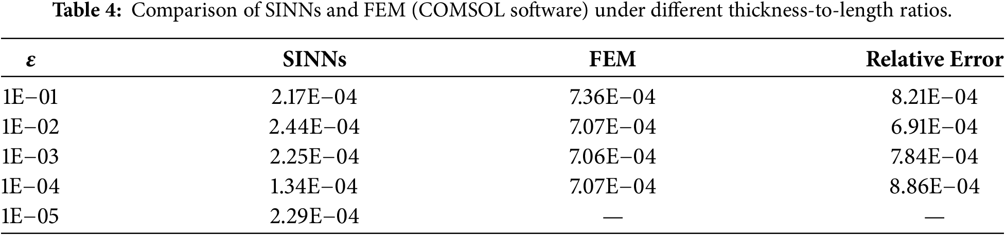
The geometry considered is a rectangular domain (Fig. 4) with a fixed width of a=0.1m and a variable length b, where the parameter b is systematically varied in the analysis. In this model, the left and lower boundaries are set to Dirichlet boundary conditions, while the right and upper boundaries are set to Neumann boundary conditions. Five Gaussian nodes are employed in conjunction with a time step of Δt=1s. Within the numerical simulations, a dimensionless parameter ε=b/a is adopted to characterize the thickness-to-length ratio. Notably, the ratio ε becomes smaller as the length b decreases. The neural network is trained by minimizing the loss function, where its architecture consists of 2 fully-connected hidden layers, each containing 20 neurons. To enhance the network’s capability of capturing oscillatory behavior, the Sinusoid function is employed. The results at t=5s are presented in Table 4, with ratios change from 10−1 to 10−5. This table presents a comparison between the results obtained from SINNs and FEM (COMSOL software). under various ratios along with the corresponding relative errors. The following observations can be drawn: The results from SINNs and FEM (COMSOL software). are generally within the same order of magnitude, indicating that SINNs can perform reliable numerical simulations for structural mechanics problems. The relative errors remain consistently around the order of 10−4. For the most extreme aspect ratio ε=10−5, the conventional FEM solver FEM (COMSOL software) requires an extremely fine mesh for very thin structures, leading to excessively long computation times and difficulties in obtaining a solution. Therefore, the method used in this study has significant advantages over traditional methods in dealing with thin-structure problems. To assess the robustness of the method in practical scenarios with measurement uncertainties, additional tests with different noise levels (0%, 1%, 3% and 5% Gaussian noise) are conducted for the most challenging case of ε=10−5. As shown in Table 5, the method exhibits remarkable stability, maintaining relative errors on the order of 10−4 even under 3% noise conditions. This indicates that the proposed approach is well-suited for real-world applications where boundary condition measurements inevitably contain noise.

3.3 Transient Heat Conduction in a Thin Toroidal Structure

As the third numerical example, this study investigates transient heat conduction in a thin toroidal structure, as illustrated in Fig. 5. The toroidal geometry is defined by an inner radius r1=0.1m and an outer radius r2, with the latter varied to represent different geometric configurations in the analysis. The governing equation, which describes the thermal behavior of the system, is formulated as follows:

ρ(⋅)c(⋅)ut(x,t)−∇[k(⋅)∇u(x,t)]=f(x,t),x∈Ω,t∈[0s,10s],(27)

where the material parameters ρ(x)c(x)=x+y, k(x)=x2+y2. The analytical temperature distribution is given as:

u(x,t)=sin⁡(t)(2x2−2y2+6xy+3x+5y).(28)

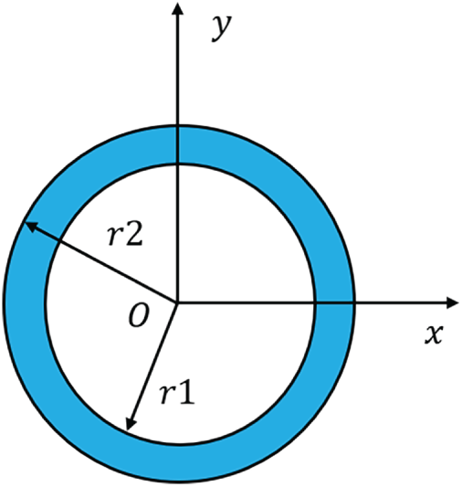
Figure 5: A thin toroidal structure.

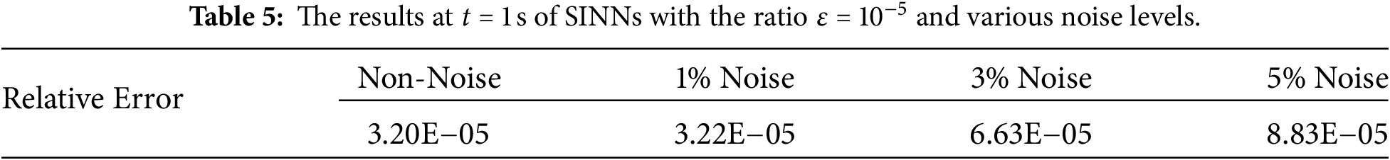
In the toroidal structure, Dirichlet boundary conditions are imposed on the outer boundary, while Neumann boundary conditions are applied to the inner boundary. A total of 350 collocation points is employed, comprising 260 boundary points and 90 interior points. For the convenience of analysis, this study defines the ratio as ε=(r2−r1)/r1. The architecture utilizes 2 fully-connected hidden layers, each consisting of 20 neurons, with the Softplus function employed as the activation function. Additionally, the number of Gaussian nodes is set to p=5, with a time step size of Δt=1s, T=5s. To comprehensively evaluate the performance of the proposed SINNs method, this study conducted verifications from both spatial and temporal dimensions. Table 6 compares the solution errors and computational times under different computational domain radii (r = 0.1 m and r = 1 m), demonstrating the robustness of the method to variations in spatial scale. For different ratios, Fig. 6 present the relative temperature errors obtained using the proposed method. The results demonstrate that the approach achieves high-precision solutions, with accuracy remaining essentially unaffected as the ratio decreases.

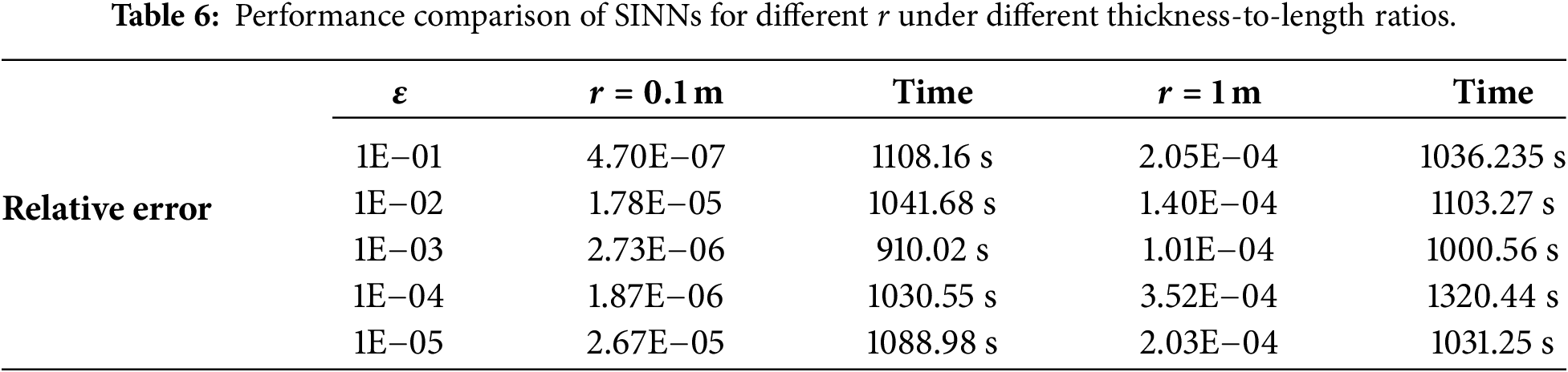
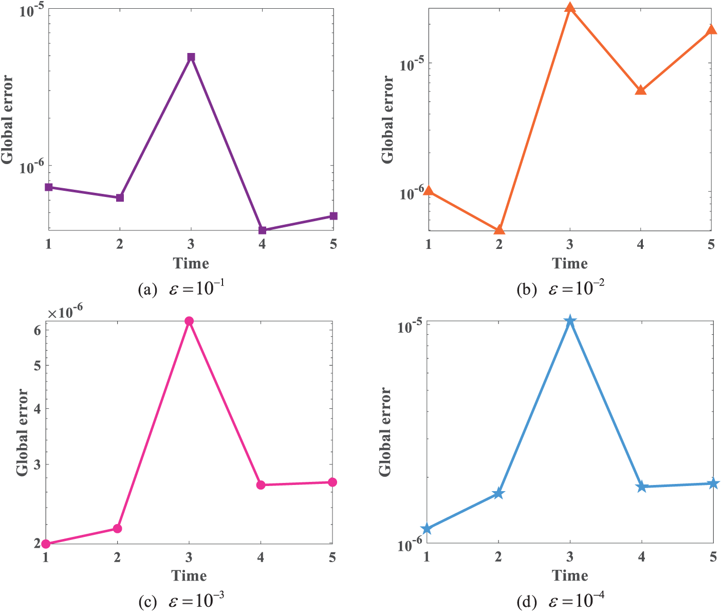
Figure 6: The global errors under different ratios from t=0 to t=5s.

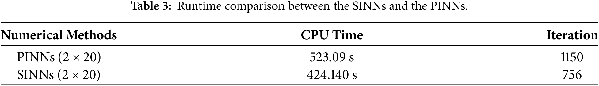
Fig. 7 presents the results obtained by PINNs and SINNs for this numerical example. In this study, large time steps of Δt=2s and Δt=4s are adopted, with the thickness-to-length ratio of the thin-walled circular ring fixed at ε=10−4. The neural network consists of 2 hidden layers, each containing 20 neurons. As can be observed, even under large time steps, SINNs are still able to maintain high accuracy and stability.

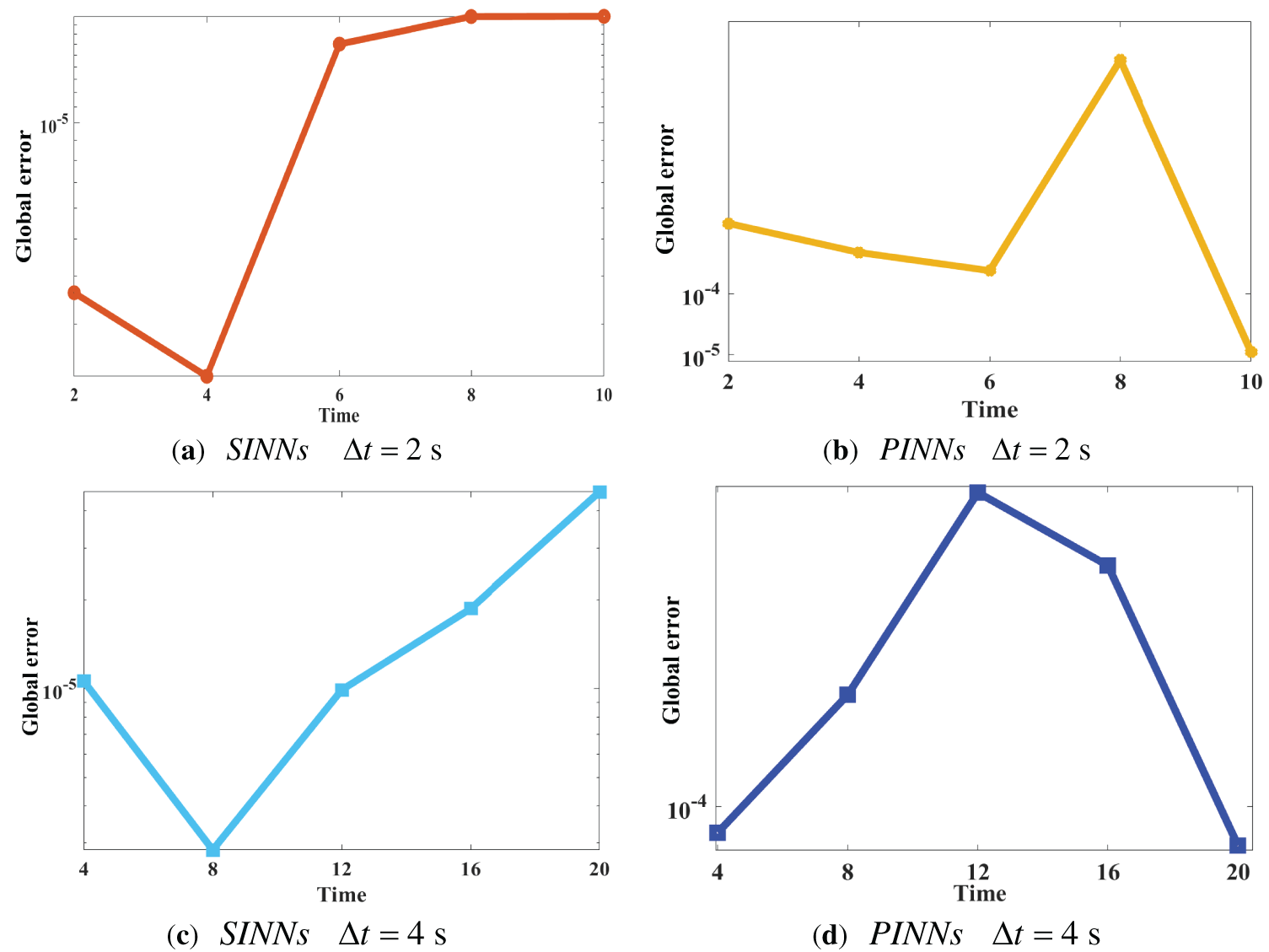
Figure 7: The global errors under different time steps between SINNs and PINNs.

3.4 Transient Heat Conduction in an Irregular-Shaped Thin-Body Domain

The final numerical example considers a heat conduction problem within an irregularly shaped thin-body domain, as illustrated in Fig. 8. The geometry of the domain is defined parametrically via Eq. (1), providing an exact mathematical description of its boundaries:

Ω={(x,y)|r2<x2+y2<(r+5×10−4)2,r=esin⁡θsin2⁡(2θ)+ecos⁡θcos2⁡(2θ)}.(29)

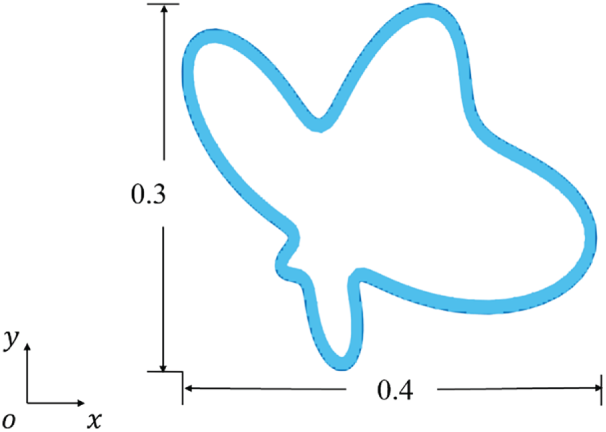
Figure 8: The configuration of an amoeba-like thin body domain.

In the aforementioned formula, the parameter θ varies between 0 and 2π.

The analytical solution is given:

u=cos⁡t(cos⁡xcosh⁡y+sin⁡xsinh⁡y).(30)

In the present example, the entire domain is represented by 2127 collocation points, with 1418 assigned to the boundary and 709 positioned within the interior domain. This study denotes the thickness of this complex geometry as h. In this complex structure, numerical simulations are performed under mixed boundary conditions, where Neumann boundary conditions are prescribed on the outer boundary and Dirichlet boundary conditions are imposed on the inner boundary.

Initially, this study specifies h=10−4 in this model. As presented in Fig. 9a, the numerical results indicate that the minimum relative error can reach 1.39×10−5. When this study set thickness of the complex domain to h=10−5, the minimum relative error is able to be 3.01×10−6 (shown in Fig. 9b). In this complex thin structure, numerical results can still maintain high accuracy, indicating that the approach works well for this irregular domain case. The results indicate that the proposed approach exhibits stable behavior, accurate predictions, for heat transfer analyses in thin bodies. To comprehensively evaluate the effectiveness of the method, a dynamic process spanning 0 s to 100 s and 0 s to 200 s is simulated, with fix h=10−5. This study selected different time steps and different time durations to verify the stability of the method. As illustrated in Fig. 10, the proposed approach demonstrates high stability and accuracy when applied to the irregular-shaped thin-body domain.

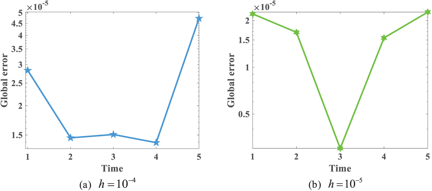
Figure 9: The global errors under different thicknesses from t=0 to t=5s.

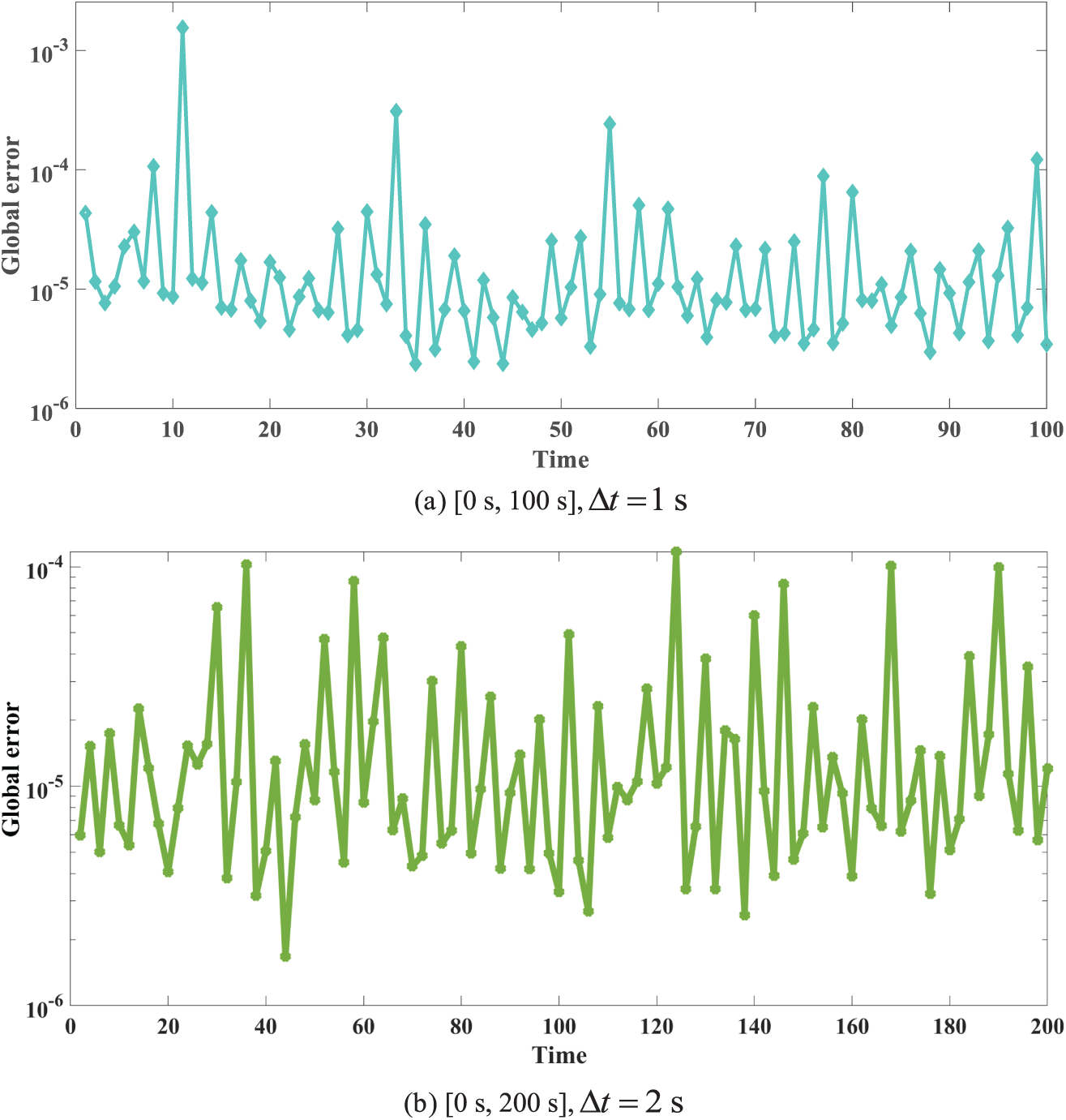
Figure 10: The global errors during the different time interval.

4  Conclusions

An integrated numerical framework based on spectral-integrated neural networks has been developed for transient heat conduction analysis in thin-body structures. By reformulating the temporal evolution through spectral integration, the proposed approach avoids the restrictive stability constraints commonly associated with conventional time-stepping schemes. As a result, accurate solutions can be obtained using comparatively large time increments, even in the presence of extreme geometric slenderness. The neural network approximation, combined with physics-based constraints, enables reliable reconstruction of both spatial temperature distributions and their temporal evolution across a wide range of thin-walled configurations. The numerical investigations demonstrate that the proposed framework remains stable and accurate for ultrathin geometries with severe aspect ratios, where traditional mesh-based methods often require excessive discretization or encounter convergence difficulties. These characteristics make the method particularly suitable for dynamic thermal analyses in thin structures, where long-time simulations and computational efficiency are critical considerations.

Several aspects merit further investigation. The current implementation is primarily validated for 2D problems, and its extension to large-scale 3D applications may introduce additional computational challenges due to increased training cost and memory requirements. Moreover, the accuracy and efficiency of the method are influenced by choices of network architecture, activation functions, and training strategies, suggesting the need for systematic or adaptive parameter selection mechanisms. Finally, while the present study focuses on linear transient heat conduction, future work will aim to extend the framework to nonlinear and coupled multiphysics problems. Potential application areas include thermal management of electronic devices and heat propagation analysis in energy storage systems.

Acknowledgement: Not applicable.

Funding Statement: The work described in this paper is supported by the National Natural Science Foundation of China (Nos. 12422207 and 12372199).

Author Contributions: Ting Gao and Chengze Shang: writing—original draft. Juan Wang: supervision, methodology. Yan Gu: writing—review & editing, funding acquisition. All authors reviewed and approved the final version of the manuscript.

Availability of Data and Materials: The data that support the findings of this study are available from the corresponding authors upon reasonable request.

Ethics Approval: Not applicable.

Conflicts of Interest: The authors declare no conflicts of interest.

References

1. Bennani HH, Takadoum J. Finite element model of elastic stresses in thin coatings submitted to applied forces. Surf Coat Technol. 1999;111(1):80–5. doi:10.1016/S0257-8972(98)00708-7. [Google Scholar] [CrossRef]

2. Cheng AHD, Cheng DT. Heritage and early history of the boundary element method. Eng Anal Bound Elem. 2005;29(3):268–302. doi:10.1016/j.enganabound.2004.12.001. [Google Scholar] [CrossRef]

3. Guiggiani M, Gigante A. A general algorithm for multidimensional Cauchy principal value integrals in the boundary element method. J Appl Mech. 1990;57(4):906–15. doi:10.1115/1.2897660. [Google Scholar] [CrossRef]

4. Chen JT, Lin SY, Chen IL, Lee YT. Mathematical analysis and numerical study to free vibrations of annular plates using BIEM and BEM. Int J Numer Methods Eng. 2006;65(2):236–63. doi:10.1002/nme.1498. [Google Scholar] [CrossRef]

5. Sladek V, Sladek J, Tanaka M. Nonsingular BEM formulations for thin-walled structures and elastostatic crack problems. Acta Mech. 1993;99(1):173–90. doi:10.1007/BF01177243. [Google Scholar] [CrossRef]

6. Zhang YM, Gu Y, Chen JT. Boundary element analysis of 2D thin walled structures with high-order geometry elements using transformation. Eng Anal Bound Elem. 2011;35(3):581–6. doi:10.1016/j.enganabound.2010.07.008. [Google Scholar] [CrossRef]

7. Gu Y, Chen W, Zhang C. Stress analysis for thin multilayered coating systems using a sinh transformed boundary element method. Int J Solids Struct. 2013;50(20–21):3460–71. doi:10.1016/j.ijsolstr.2013.06.018. [Google Scholar] [CrossRef]

8. Gu Y, Sun L. Electroelastic analysis of two-dimensional ultrathin layered piezoelectric films by an advanced boundary element method. Int J Numer Methods Eng. 2021;122(11):2653–71. doi:10.1002/nme.6635. [Google Scholar] [CrossRef]

9. Wang F, Chen W, Gu Y. Boundary element analysis of inverse heat conduction problems in 2D thin-walled structures. Int J Heat Mass Transf. 2015;91(3):1001–9. doi:10.1016/j.ijheatmasstransfer.2015.08.048. [Google Scholar] [CrossRef]

10. Zhou H, Niu Z, Cheng C, Guan Z. Analytical integral algorithm applied to boundary layer effect and thin body effect in BEM for anisotropic potential problems. Comput Struct. 2008;86(15–16):1656–71. doi:10.1016/j.compstruc.2007.10.002. [Google Scholar] [CrossRef]

11. Liu Y, Fan H. On the conventional boundary integral equation formulation for piezoelectric solids with defects or of thin shapes. Eng Anal Bound Elem. 2001;25(2):77–91. doi:10.1016/S0955-7997(01)00004-2. [Google Scholar] [CrossRef]

12. Krishnasamy G, Rizzo FJ, Liu Y. Boundary integral equations for thin bodies. Int J Numer Methods Eng. 1994;37(1):107–21. doi:10.1002/nme.1620370108. [Google Scholar] [CrossRef]

13. Fu ZJ, Zhang J, Li PW, Zheng JH. A semi-Lagrangian meshless framework for numerical solutions of two-dimensional sloshing phenomenon. Eng Anal Bound Elem. 2020;112(5):58–67. doi:10.1016/j.enganabound.2019.12.003. [Google Scholar] [CrossRef]

14. Fu Z, Chen W, Wen P, Zhang C. Singular boundary method for wave propagation analysis in periodic structures. J Sound Vib. 2018;425:170–88. doi:10.1016/j.jsv.2018.04.005. [Google Scholar] [CrossRef]

15. Gu Y, Fan CM, Fu Z. Localized method of fundamental solutions for three-dimensional elasticity problems: theory. Adv Appl Math Mech. 2021;13(6):1520–34. doi:10.4208/aamm.oa-2020-0134. [Google Scholar] [CrossRef]

16. Chen CS, Cho HA, Golberg MA. Some comments on the ill-conditioning of the method of fundamental solutions. Eng Anal Bound Elem. 2006;30(5):405–10. doi:10.1016/j.enganabound.2006.01.001. [Google Scholar] [CrossRef]

17. Fu Z, Chen W. A truly boundary-only meshfree method applied to Kirchhoff plate bending problems. Adv Appl Math Mech. 2009;1(3):341–52. doi:10.1007/s00466-009-0411-6. [Google Scholar] [CrossRef]

18. Chen CS, Jiang X, Chen W, Yao G. Fast solution for solving the modified Helmholtz equation withthe method of fundamental solutions. Commun Comput Phys. 2015;17(3):867–86. doi:10.4208/cicp.181113.241014a. [Google Scholar] [CrossRef]

19. Zobeiry N, Humfeld KD. A physics-informed machine learning approach for solving heat transfer equation in advanced manufacturing and engineering applications. Eng Appl Artif Intell. 2021;101:104232. doi:10.1016/j.engappai.2021.104232. [Google Scholar] [CrossRef]

20. Raissi M, Perdikaris P, Karniadakis GE. Physics-informed neural networks: a deep learning framework for solving forward and inverse problems involving nonlinear partial differential equations. J Comput Phys. 2019;378:686–707. doi:10.1016/j.jcp.2018.10.045. [Google Scholar] [CrossRef]

21. Wang S, Teng Y, Perdikaris P. Understanding and mitigating gradient flow pathologies in physics-informed neural networks. SIAM J Sci Comput. 2021;43(5):A3055–81. doi:10.1137/20m1318043. [Google Scholar] [CrossRef]

22. Karniadakis GE, Kevrekidis IG, Lu L, Perdikaris P, Wang S, Yang L. Physics-informed machine learning. Nat Rev Phys. 2021;3(6):422–40. doi:10.1038/s42254-021-00314-5. [Google Scholar] [CrossRef]

23. Tang Z, Fu Z, Reutskiy S. An extrinsic approach based on physics-informed neural networks for PDEs on surfaces. Mathematics. 2022;10(16):2861. doi:10.3390/math10162861. [Google Scholar] [CrossRef]

24. Zhang B, Wu G, Gu Y, Wang X, Wang F. Multi-domain physics-informed neural network for solving forward and inverse problems of steady-state heat conduction in multilayer media. Phys Fluids. 2022;34(11):116116. doi:10.1063/5.0116038. [Google Scholar] [CrossRef]

25. Lu L, Pestourie R, Yao W, Wang Z, Verdugo F, Johnson SG. Physics-informed neural networks with hard constraints for inverse design. SIAM J Sci Comput. 2021;43(6):B1105–32. doi:10.1137/21m1397908. [Google Scholar] [CrossRef]

26. He Q, Barajas-Solano D, Tartakovsky G, Tartakovsky AM. Physics-informed neural networks for multiphysics data assimilation with application to subsurface transport. Adv Water Resour. 2020;141(2):103610. doi:10.1016/j.advwatres.2020.103610. [Google Scholar] [CrossRef]

27. Gu Y, Zhang C, Zhang P, Golub MV, Yu B. Enriched physics-informed neural networks for 2D in-plane crack analysis: theory and MATLAB code. Int J Solids Struct. 2023;276(1):112321. doi:10.1016/j.ijsolstr.2023.112321. [Google Scholar] [CrossRef]

28. Rezaei S, Harandi A, Moeineddin A, Xu BX, Reese S. A mixed formulation for physics-informed neural networks as a potential solver for engineering problems in heterogeneous domains: comparison with finite element method. Comput Methods Appl Mech Eng. 2022;401(1):115616. doi:10.1016/j.cma.2022.115616. [Google Scholar] [CrossRef]

29. Kissas G, Yang Y, Hwuang E, Witschey WR, Detre JA, Perdikaris P. Machine learning in cardiovascular flows modeling: predicting arterial blood pressure from non-invasive 4D flow MRI data using physics-informed neural networks. Comput Methods Appl Mech Eng. 2020;358(1):112623. doi:10.1016/j.cma.2019.112623. [Google Scholar] [CrossRef]

30. Misyris GS, Venzke A, Chatzivasileiadis S. Physics-informed neural networks for power systems. In: Proceedings of the 2020 IEEE Power & Energy Society General Meeting (PESGM); 2020 Aug 2–6; Montreal, QC, Canada. p. 1–5. doi:10.1109/pesgm41954.2020.9282004. [Google Scholar] [CrossRef]

31. Nascimento RG, Corbetta M, Kulkarni CS, Viana FAC. Hybrid physics-informed neural networks for lithium-ion battery modeling and prognosis. J Power Sources. 2021;513(1):230526. doi:10.1016/j.jpowsour.2021.230526. [Google Scholar] [CrossRef]

32. Samaje P, Salma A, Venkadeshwaran K, Varma SVK, Hanumagowda BN, Verma A, et al. A comparative analysis on the magnetohydrodynamic mixed convective flow of a hybrid nanofluid with radiative heat transfer using bagging regression. Int J Ambient Energy. 2024;45(1):2386045. doi:10.1080/01430750.2024.2386045. [Google Scholar] [CrossRef]

33. Jagtap AD, Kharazmi E, Karniadakis GE. Conservative physics-informed neural networks on discrete domains for conservation laws: applications to forward and inverse problems. Comput Methods Appl Mech Eng. 2020;365(1):113028. doi:10.1016/j.cma.2020.113028. [Google Scholar] [CrossRef]

34. Pang G, Lu L, Karniadakis GE. fPINNs: fractional physics-informed neural networks. SIAM J Sci Comput. 2019;41(4):A2603–26. doi:10.1137/18m1229845. [Google Scholar] [CrossRef]

35. Linka K, Schäfer A, Meng X, Zou Z, Karniadakis GE, Kuhl E. Bayesian physics informed neural networks for real-world nonlinear dynamical systems. Comput Methods Appl Mech Eng. 2022;402(9):115346. doi:10.1016/j.cma.2022.115346. [Google Scholar] [CrossRef]

36. Kharazmi E, Zhang Z, Karniadakis GEM. hp-VPINNs: variational physics-informed neural networks with domain decomposition. Comput Methods Appl Mech Eng. 2021;374(1):113547. doi:10.1016/j.cma.2020.113547. [Google Scholar] [CrossRef]

37. Chandan K, Saadeh R, Qazza A, Karthik K, Varun Kumar RS, Kumar RN, et al. Predicting the thermal distribution in a convective wavy fin using a novel training physics-informed neural network method. Sci Rep. 2024;14(1):7045. doi:10.1038/s41598-024-57772-x. [Google Scholar] [PubMed] [CrossRef]

38. Gu Y, Zhang C, Golub MV. Physics-informed neural networks for analysis of 2D thin-walled structures. Eng Anal Bound Elem. 2022;145(5):161–72. doi:10.1016/j.enganabound.2022.09.024. [Google Scholar] [CrossRef]

39. Qiu L, Wang F, Qu W, Gu Y, Qin QH. Spectral integrated neural networks (SINNs) for solving forward and inverse dynamic problems. Neural Netw. 2024;180:106756. doi:10.1016/j.neunet.2024.106756. [Google Scholar] [PubMed] [CrossRef]

40. Ma H, Qu W, Gu Y, Qiu L, Wang F, Zhao S. Spectral integrated neural networks with large time steps for 2D and 3D transient elastodynamic analysis. Neural Netw. 2025;188:107559. doi:10.1016/j.neunet.2025.107559. [Google Scholar] [PubMed] [CrossRef]

41. Qu W, Gu Y, Zhang Y, Fan CM, Zhang C. A combined scheme of generalized finite difference method and Krylov deferred correction technique for highly accurate solution of transient heat conduction problems. Int J Numer Methods Eng. 2019;117(1):63–83. doi:10.1002/nme.5948. [Google Scholar] [CrossRef]

42. Atilim GB, Barak AP, Alexey AR, Jeffrey MS. Automatic differentiation in machine learning: a survey. arXiv:1502.05767. 2015. [Google Scholar]

43. Qiu L, Lin J, Wang F, Qin QH, Liu CS. A homogenization function method for inverse heat source problems in 3D functionally graded materials. Appl Math Model. 2021;91:923–33. doi:10.1016/j.apm.2020.10.012. [Google Scholar] [CrossRef]

44. Yang K, Jiang GH, Li HY, Zhang ZB, Gao XW. Element differential method for solving transient heat conduction problems. Int J Heat Mass Transf. 2018;127:1189–97. doi:10.1016/j.ijheatmasstransfer.2018.07.155. [Google Scholar] [CrossRef]

45. Sun W, Ma H, Qu W. A hybrid numerical method for non-linear transient heat conduction problems with temperature-dependent thermal conductivity. Appl Math Lett. 2024;148:108868. doi:10.1016/j.aml.2023.108868. [Google Scholar] [CrossRef]

46. Huang J, Jia J, Minion M. Arbitrary order Krylov deferred correction methods for differential algebraic equations. J Comput Phys. 2007;221(2):739–60. doi:10.1016/j.jcp.2006.06.040. [Google Scholar] [CrossRef]

47. Jia J, Huang J. Krylov deferred correction accelerated method of lines transpose for parabolic problems. J Comput Phys. 2008;227(3):1739–53. doi:10.1016/j.jcp.2007.09.018. [Google Scholar] [CrossRef]