Modeling of the Separation Bubble on Cambered Airfoils Utilizing Modified Parameters in a Transition Model

1  Introduction

Laminar separation bubbles (LSBs) represent a significant phenomenon in aerodynamics, occurring when the laminar boundary layer separates from a surface due to an adverse pressure gradient and reattaches further downstream as a turbulent boundary layer [1]. This separation and reattachment form a bubble-like structure that has profound effects on aerodynamic performance, influencing lift, drag, and flow stability [2,3]. At low Reynolds (Re) numbers (Re~104–105), viscous forces are more dominant than inertial forces. Understanding LSBs is critical for low-Re number aerodynamics, unmanned aerial vehicles, wind turbines, and other applications where viscous forces play a dominant role [4].

The physical mechanisms of LSB involve a delicate coupling between separation, transition, and reattachment processes, often governed by Tollmien–Schlichting wave amplification and Kelvin–Helmholtz instabilities inside the separated shear layer [5]. The size, location, and stability of LSBs are strongly dependent on Reynolds number, angle of attack, free-stream turbulence, and airfoil geometry, especially the thickness distribution [6]. Thicker wing profiles generally improve lift generation at lower speeds but tend to increase drag, thus reducing aerodynamic efficiency [6,7]. Conversely, altering the camber can significantly impact the pressure distribution over the wing, affecting lift generation and the wing’s stall behavior. Ayvazoğlu et al. [7] studied cambered profiles with variable thickness and reported that thicker airfoils exhibited long bubbles due to stronger adverse pressure gradients. It was observed that the lift and drag coefficients increased as the thickness increased. Oil-flow visualization confirmed that the bubbles shortened and moved toward the leading edge with increasing angle or inertial forces. Comparison with numerical results revealed delayed separation predictions, indicating that the k–ω SST Transition model requires additional empirical correlations for accurate low-Re flow prediction.

Numerical and experimental studies on LSBs have provided valuable insights into their formation, dynamics, and control for decades. Computational Fluid Dynamics (CFD) has been widely used to simulate LSB behavior, offering detailed flow field data and enabling parametric studies under controlled conditions. Giacomini and Westerberg [8] showed that employing transition-capable models in FLUENT markedly improves lift and drag predictions by capturing laminar separation bubble behaviour. Similarly, Matsson et al. [9] found that transition-sensitive modeling better correlates with experimental stall onset in NACA 2412. Carreño Ruiz and D’Ambrosio [10] validated various γ–Reθ empirical correlations and identified those that most reliably predict separation, transition, and reattachment in low-Re airfoils. Liu et al. [11] compared multiple transition models and highlighted their sensitivity to mesh and solver settings. Michna and Rogowski [12] observed that small changes in Reynolds number or inlet turbulence intensity can significantly alter lift and drag coefficients in NACA 0018 simulations. High-fidelity Direct Numerical Simulation (DNS) work by Klose et al. [13] on cambered airfoils at Re = 0.2 × 105 offered valuable insight into bubble dynamics, serving as a reference for CFD validation. Michna et al. [14] investigated harmonically pitching airfoils and revealed strong hysteresis and bubble oscillations in low-Re regimes. Tanürün et al. [15] further demonstrated that surface roughness alters transition location and stall behaviour, underscoring the importance of operational surface conditions. Collectively, these findings highlight the necessity of transition modeling, refined meshing strategies, and geometry optimization for accurate low-Reynolds-number simulations. Tangermann and Klein [16] have studied the numerical analysis of the NACA 0018 symmetric airfoil using Reynolds Average Navier Stokes (RANS) and Large Eddy Simulation (LES) models at 4° and 8° angles of attack. They have investigated the laminar separation bubble in various cases for the free-stream turbulence intensity in ambient turbulence. It has been observed that the effect of free-stream turbulence is largely dependent on the length scale. The turbulence length scale quantifies the characteristic dimensions of energy-dominant turbulent structures and is essential for the representation of turbulent transport processes and flow modeling.

Experimental investigations complement numerical studies by providing physical validation and practical insights into LSB behavior. Most studies have focused on examining how variations in Reynolds number, turbulence intensity, and streamwise pressure gradient influence bubble dynamics [17–20]. Samson and Sarkar [21] showed that at low free-stream turbulence (FST), the transition in a leading-edge separation bubble occurs through Kelvin–Helmholtz instability, while at higher turbulence levels it shifts to a bypass mode driven by transient disturbance growth. Increasing both FST and Reynolds number shortened the bubble, with FST having the stronger influence. Kumar and Sarkar [22] investigated the evolution and breakdown of LSBs under adverse pressure gradients. Using experiments and LES at Re = 2 × 105 and 1% FST, it was found that stronger pressure gradients shift transition upstream and shorten bubble length. Early flow features show Kelvin–Helmholtz vortices that amplify disturbances, while LES results reveal inviscid–viscous interactions driving shear-layer breakdown and transition to turbulence. Açıkel and Serdar Genç [23] conducted experiments on a NACA 4412 airfoil at low Reynolds numbers, integrating a partially flexible membrane to measure aerodynamic forces across various angles of attack and Reynolds numbers. To better visualize flow separation and LSB formation, they utilized smoke visualization and hot-wire anemometry. The experiments revealed that the location and formation of the LSB were influenced by variations in Reynolds number and angle of attack. Low angles of attack denote pre-stall conditions between α = 0° and α = 8°, whereas moderate (α = 8°–10°) and high angles of attack (α = 12°–15°) correspond to near-stall and post-stall conditions, respectively. At low angles of attack, shorter bubbles formed, leading to an increased number of vortices. In contrast, at moderate angles of attack, longer bubbles were observed, but with decreased vortex frequency. The study concluded that LSBs could induce vibration and noise in wind turbine blades, necessitating a comprehensive understanding and elimination of LSBs to enhance aerodynamic performance and energy efficiency. Boutilier and Yarusevych [24] studied the shear layer development on the NACA 0018 airfoil at 1 × 105 Reynolds number from the angles of attack of 0° to 15° using a combination of smoke test from flow visualization techniques, hot-wire surface velocity field mapping from surface velocity measurement techniques, surface pressure fluctuation measurements, and stability analysis. The experimental results together described the transition in the shear layer at low Re numbers. The experiments also showed the magnitude of flow separation, reattachment, and adhesion velocity. Therefore, the claim that the measured convective velocities of the fluid separated in the shear layer are related to the waves of increasing disturbances has been proven.

Although the understanding of laminar separation bubbles has advanced significantly through both experimental and numerical studies, their accurate numerical prediction remains a formidable challenge [25]. One approach involves incorporating low-Reynolds-number modifications to control turbulence generation during the onset of transition. These formulations typically introduce damping functions to account for the reduced turbulence activity within the viscous sublayer. Although various low-Reynolds-number turbulence models have been proposed over the years [26–28], their ability to predict transition remains largely empirical and unreliable [29]. Another common strategy involves representing the transition region as a combination of laminar and turbulent flow components, weighted by an intermittency factor (γ). This parameter varies between 0 and 1, where γ = 0 indicates a completely laminar state, and γ = 1 corresponds to a fully turbulent flow [30]. To effectively implement this approach, empirical correlations are required to determine both the transition onset location and the streamwise development of γ. These correlations typically relate the momentum-thickness-based transition Reynolds number (Reθt) to local flow variables such as turbulence intensity (Tu) and the pressure-gradient parameter (λ). Early models for laminar–turbulent transition primarily relied on empirical correlations and intermittency transport equations. For instance, Mayle [31] suggested correlations for zero-pressure-gradient flows, relating the transition onset to Tu and momentum thickness (θ), while later, Gostelow et al. [32] extended this approach to describe how intermittency evolves along the flow direction using local parameters such as Tu, θ, and the λ. Throughout the 1990s, researchers developed methods to integrate intermittency transport equations with classical two-equation turbulence models, allowing the turbulent production term to be modulated based on the transitional state [33,34]. Building on these earlier studies, Menter introduced a transition model based on local flow variables and subsequently coupled it with the SST k–ω turbulence model to form the γ–Reθt transition model [35]. By relying on local rather than nonlocal flow properties, this model provides a more robust and physics-based framework for predicting laminar separation bubbles and the transition process. However, when compared with experimental results, particularly at low Reynolds numbers, the model does not always fully capture the onset and extent of laminar separation bubbles. Small discrepancies in the predicted bubble length, location, and transition behavior highlight the sensitivity of the model to the empirical parameters Reθt and Reθc. These limitations indicate a need for further refinement and calibration of the model to improve its predictive accuracy for low-Reynolds-number airfoils, which is the primary focus of the present study.

The present study aims to investigate the dynamics of LSBs and the transition process over NACA 24xx family airfoils at Reynolds numbers of 0.5 × 105, 1.5 × 105, and 2.5 × 105 and angles of attack of 0°, 4°, and 8°, under a low free-stream turbulence intensity (<1%) using a combined numerical and experimental approach. The analysis focuses on how the empirical parameters within the transition-sensitive model (γ–Reθt Transition SST) influence bubble formation, transition onset, and the overall flow behavior. High-fidelity numerical simulations are performed in ANSYS FLUENT, where the Transition SST model incorporates local flow variables and governing equations for intermittency transport to capture the effects of laminar separation and turbulent reattachment directly. The impact of the empirical parameters, notably Reθt and Reθc, on bubble length, position, and transition onset is analysed, considering their critical role in LSB prediction. Complementary wind tunnel experiments, including glue-on shear stress measurements and oil-film visualization, are used to validate the numerical predictions. A selection of NACA 2412, NACA 2415, and NACA 2418 airfoils is considered to examine how airfoil thickness affects LSB formation and transition behavior. Detailed analyses of velocity fields, intermittency distribution, and turbulence production provide deeper insight into bubble dynamics, while also highlighting the limitations of current transition models at low Reynolds numbers. This integrated approach not only clarifies the influence of Reθt and Reθc on LSB prediction but also guides potential refinements in transition modeling for low-Re airfoils.

2  Materials and Methods

2.1 Numerical Simulation Details

In this study, numerical modeling of LSB occurring at low Reynolds numbers on cambered airfoils was performed by using ANSYS FLUENT. The main objective is to model the LSB formation using the transition model more accurately. The model utilizes user-defined functions to modify the empirical equations employed in the transition model, thereby enabling more accurate simulations. The SST-Transition model, a turbulence model frequently used in turbulent transition modeling studies and reported in the literature to yield better results than other turbulence models at low Reynolds numbers, was used in the numerical modeling. Compared to fully turbulent models, the SST-Transition model improves the prediction of aerodynamic performance by providing more accurate estimation of skin friction, separation and transition onset, and reattachment locations. Its capability to capture transition physics makes it especially suitable for external aerodynamics, turbomachinery, and low-Reynolds-number applications, where transitional phenomena have a significant influence on overall flow behavior.

The study attempted to identify the LSB locations on the airfoil at Reynolds numbers of 0.5 × 105, 1.5 × 105, and 2.5 × 105 and at different angles of attack. Fig. 1 shows the flow field and mesh structure created for the numerical model. The numerical modeling was performed in 2D, and the mesh structure was created accordingly. During the numerical study, the wall y+ value was kept less than 1, and mesh independence study was performed to ensure that the results obtained from the model were independent of the mesh structure. The results of the mesh independence study are presented in Fig. 2. For the grid independence study, numerical modeling was performed with varying mesh numbers ranging from approximately 90,000 to 400,000. Based on the results, since there was no significant change in aerodynamic force coefficients after a mesh number of 310,000, this number was chosen and the analyses were conducted using this mesh number.

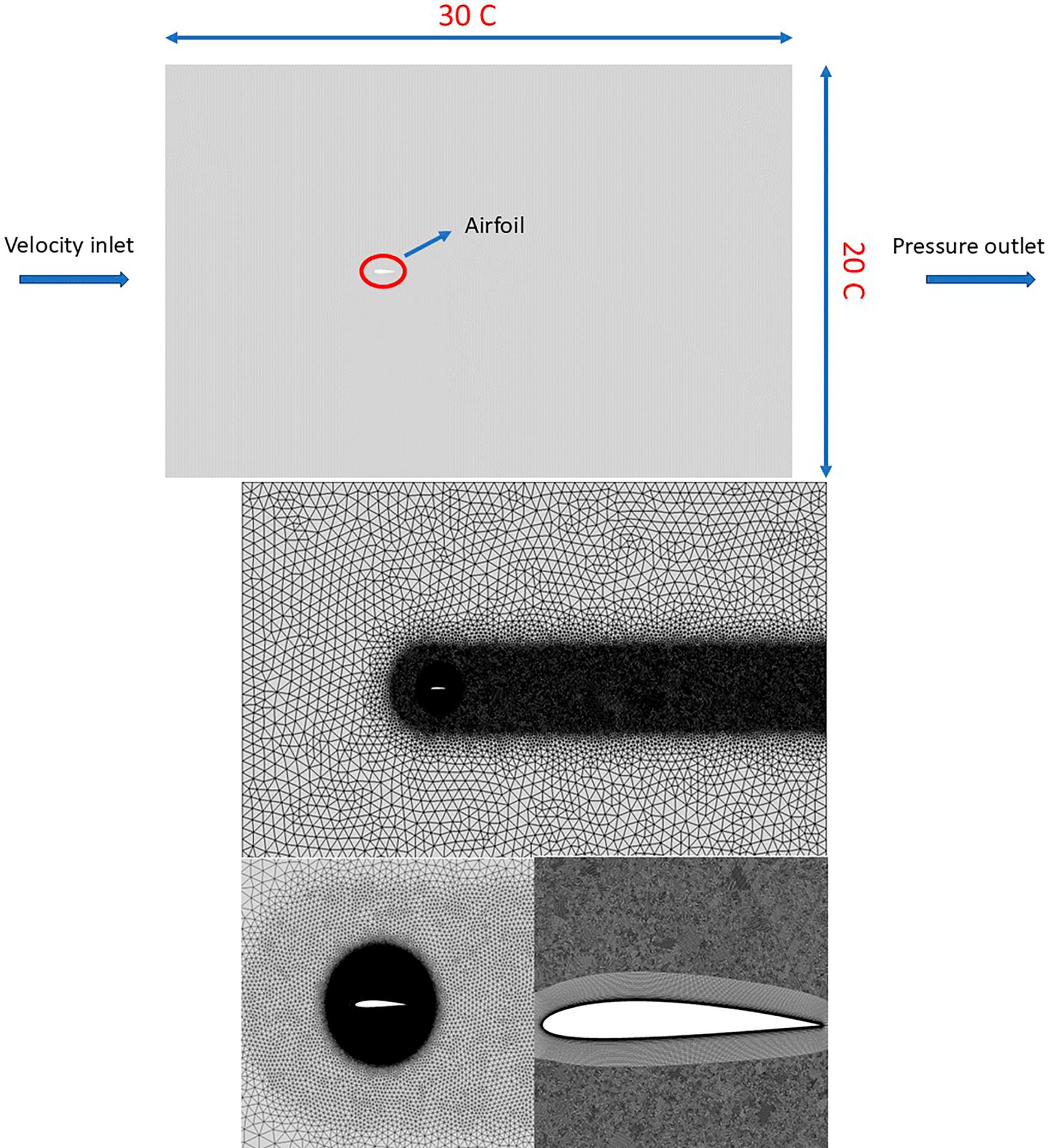
Figure 1: Flow domain of numerical model.

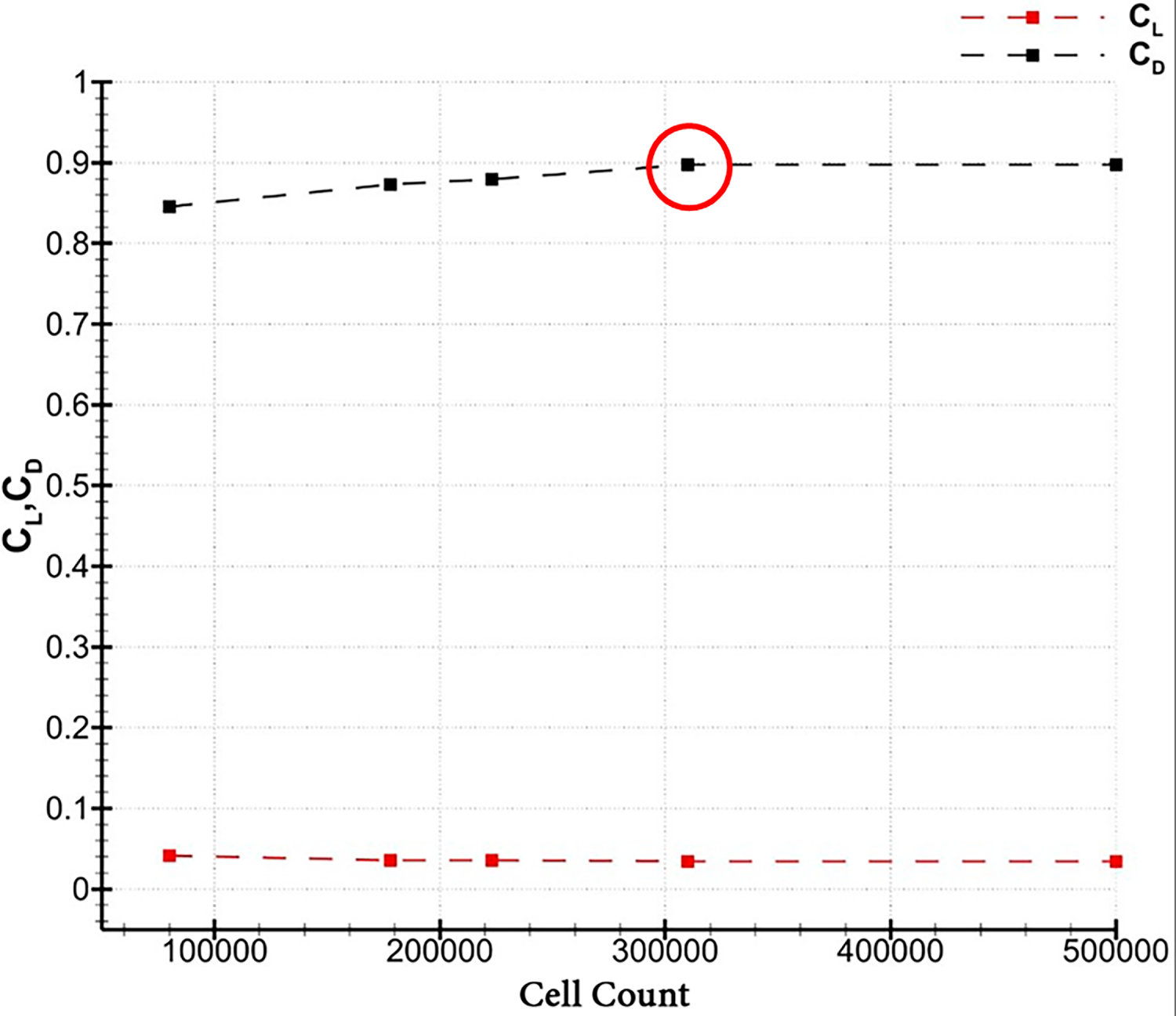
Figure 2: The grid independence study for numerical simulation.

2.2 Experimental Setup Details for Validation

All experimental activities were conducted in the suction-type open-circuit wind tunnel shown in Fig. 3a, located in the Wind Engineering and Aerodynamic Research Laboratory (WEAR) of the Department of Energy Systems Engineering at Erciyes University. The general characteristics of the suction-type wind tunnel are as follows: it features a transparent test section measuring 50 cm × 50 cm, constructed from plexiglas material to facilitate visualization techniques. The tunnel’s minimum air speed is 3 m/s, while the maximum air speed reaches 40 m/s. Additionally, the turbulence intensity at maximum speed is well below 1% [36]. Fig. 3b shows a schematic representation of the wind tunnel.

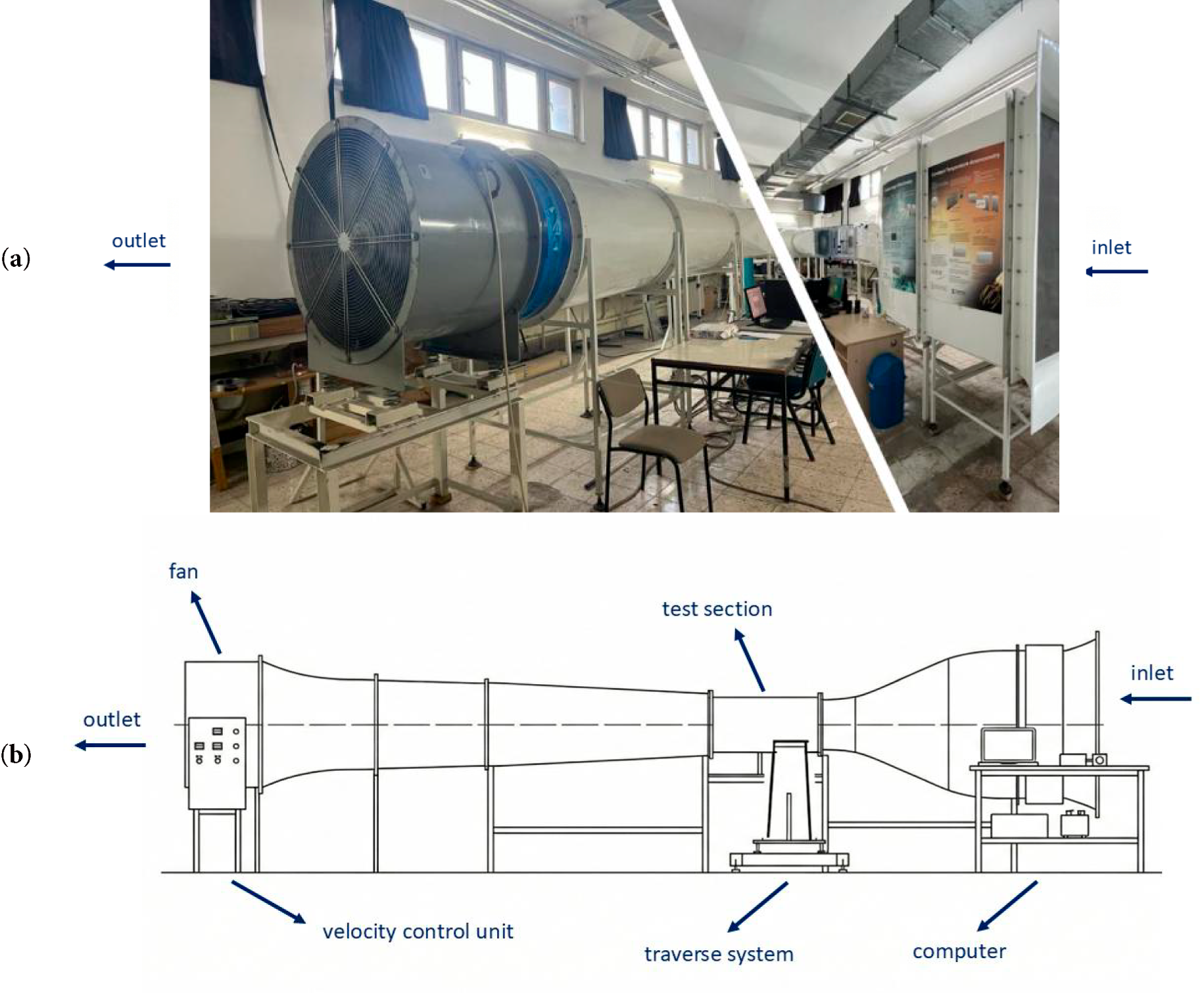
Figure 3: (a) The suction type wind tunnel used for experiments at the WEAR Laboratory and (b) The schematic of the wind tunnel.

The chord length of the airfoil profiles utilized for the studies is 180 mm, with a span length is 300 mm. The airfoil design implemented in the SOLIDWORKS program is given in Fig. 4a.

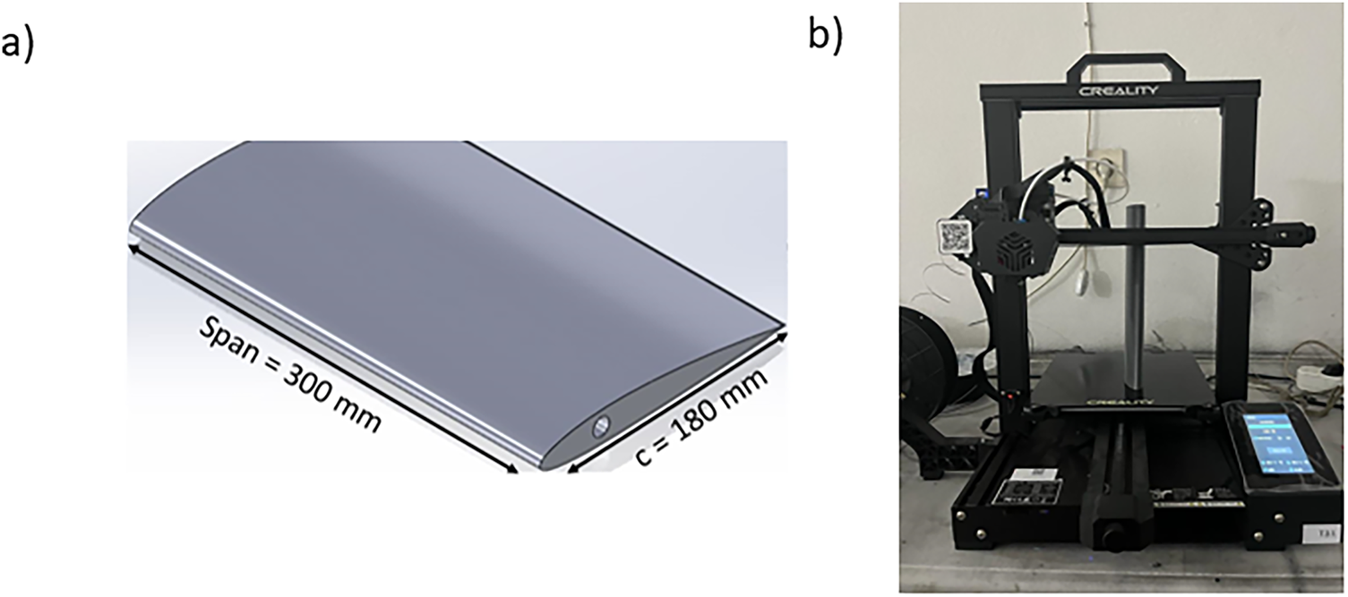
Figure 4: (a) Geometric dimensions of the airfoil (b) 3D printer (c) Manufacturing process of the airfoil used in the experiments.

The airfoils used in the experiments were produced using a Creality Ender-3 Pro brand 3D printer (Fig. 4b). The airfoils were made of polylactic acid (PLA) material. Surface defects of the produced airfoils were removed by sanding and then painted and varnished to prepare them for the experiment (Fig. 4c).

A flow visualization experiment was performed by applying an oil mixture to the surface, which is a simple and inexpensive method that allows us to observe the flow conditions occurring on the surface, which is frequently used in aerodynamic analyses [14,37–39]. In the oil flow visualization experiment, a mixture is prepared using machine oil, titanium dioxide, and kerosene. This mixture is applied homogeneously to the airfoil surface using a brush. Then, the airfoil is exposed to the flow to create flow patterns. The resulting flow patterns provide information about the flow separations that occur on the airfoil. Once the flow patterns formed on the airfoil surface stabilize, they are photographed in an attempt to understand the flow structure over the airfoil. In order to take images of the experiment, the camera system is positioned in the tunnel with the help of a tripod. Fig. 5 shows an example of the flow pattern formed before and after the oil flow visualization experiment. Fig. 5a illustrates the condition in which no flow is present over the airfoil, whereas Fig. 5b depicts the case where the flow over the airfoil is consistent.

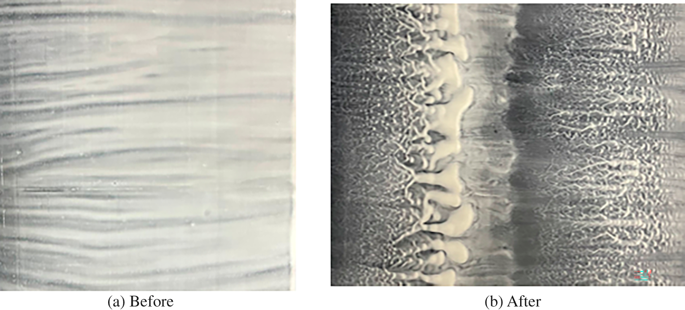
Figure 5: Before (a) and after (b) flow visualization experiment by using an oil mixture.

An experiment was conducted to measure surface shear stress using a Glue-on probe (Fig. 6) to quantitatively analyze surface flow phenomena. The literature regarding this experiment does not mention the calibration of the glue-on probe due to its complexity. Therefore, the experimental process was completed by processing the time-dependent voltage data obtained from the probe at different points along the chord on the wing surface. The equation defined by Zhang et al. [40] uses quasi-shear stress to express the boundary layer separations, transition region and flow reattachment to the surface on the airfoil.

τ=(E2−E02E02)3(1)

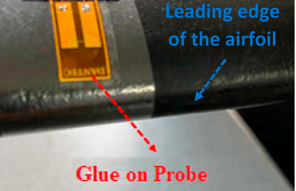
Figure 6: The glue-on probe is placed on the airfoil surface near the leading edge [41].

Eq. (1), E represents the voltage value measured when there is flow over the probe, while E0 represents the voltage value measured when there is no flow over the probe. The DANTEC 55R47 coded probe was used in the experiments. In this study, glue-on experiments were performed to examine the flow events occurring on airfoils with different thickness and camber in more detail. The main goal here is to examine the effect of the flow conditions occurring on the airfoil surface through shear stress. In this experimental method, since it is difficult to perform the calibration process, the voltage data obtained were used. By drawing time-dependent graphs of the voltage data obtained by taking 1024 data per second at each x/c point, boundary layer separations, unstable flow region and retention of the flow on the surface by passing into turbulence were investigated. Fig. 7 shows the voltage change taken point by point on the chord length depending on time at 1.5 × 105 Re number at the angle of attack of 4°. These measurements were between 0.05 and 0.85 chord length. Due to the probe support cable connection, experiments were taken to a maximum of x/c (distance from the leading edge) = 0.85. When the time-dependent voltage variation is examined, an increase in the amplitude of fluctuations is started at the point of x/c = 0.3. These fluctuations indicate to start of the transition. However, the transition onset is newly started, and 3D fluctuations will occur after 2D flow fluctuations. The oscillation and increase in voltage fluctuations manifest the formation of these. Beyond x/c = 0.7, the time-dependent data reveal an increase in the characteristic wavelengths due to the completion of the transition to turbulence. Downstream of this location, the flow is observed to undergo a transition and subsequently reattach to the surface.

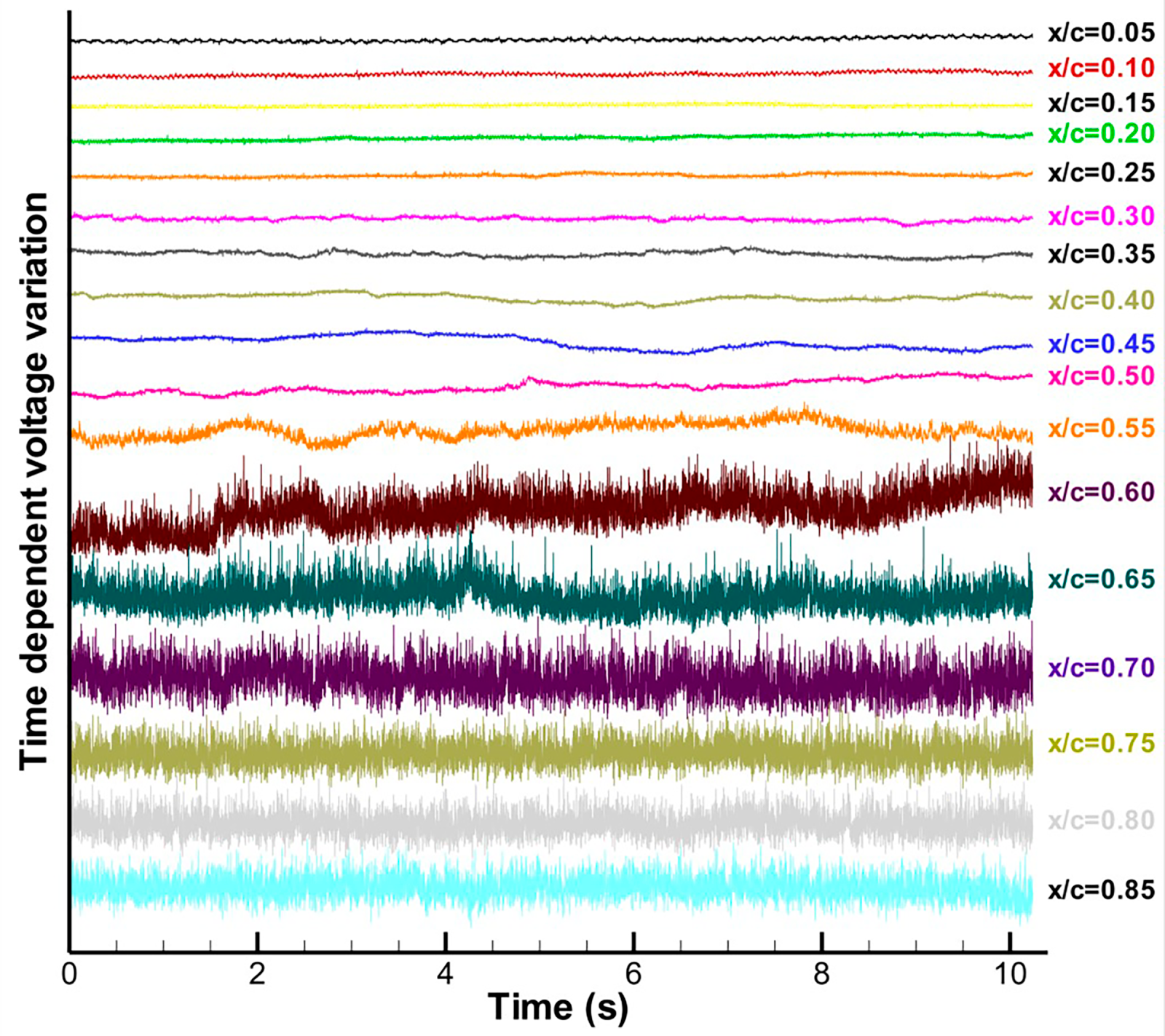
Figure 7: Time-dependent voltage variation from NACA 2415 at α = 4° and Re = 1.5 × 105.

2.3 Experimental Results

Viscous effects cause the boundary layer to separate from the airfoil surface and reattach after undergoing transition in the shear layer over the surface, forming a separation bubble [23,31]. Experiments were carried out by applying the prepared oil mixture to the suction surface of the airfoil [41]. The results obtained from the experiments are given in Figs. 8–10. For the NACA 2412 airfoil at the angle of attack of 0° and a Reynolds number of 0.5 × 105 (Fig. 8A1), results from the oil flow experiment indicated that the flow separates at x/c = 0.44 and does not reattach to the surface. At a higher Reynolds number of 1.5 × 105 (Fig. 8B2), the flow separates closer to the leading edge at x/c = 0.30, but the transition forms at x/c = 0.70, allowing it to reattach to the airfoil surface.

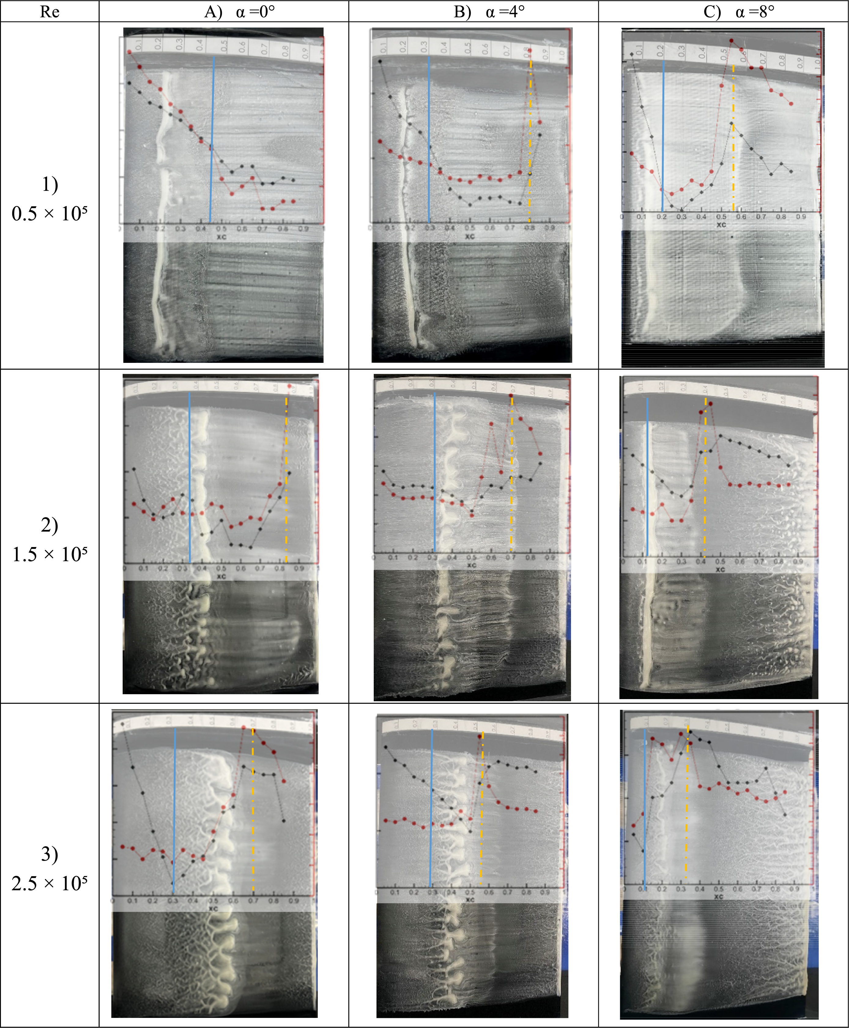
Figure 8: Comparison of oil test results with voltage (black line)-standard deviation (red line) changes at different angles of attack and Re numbers of NACA 2412 airfoil (blue line: separation point, orange line: transition point).

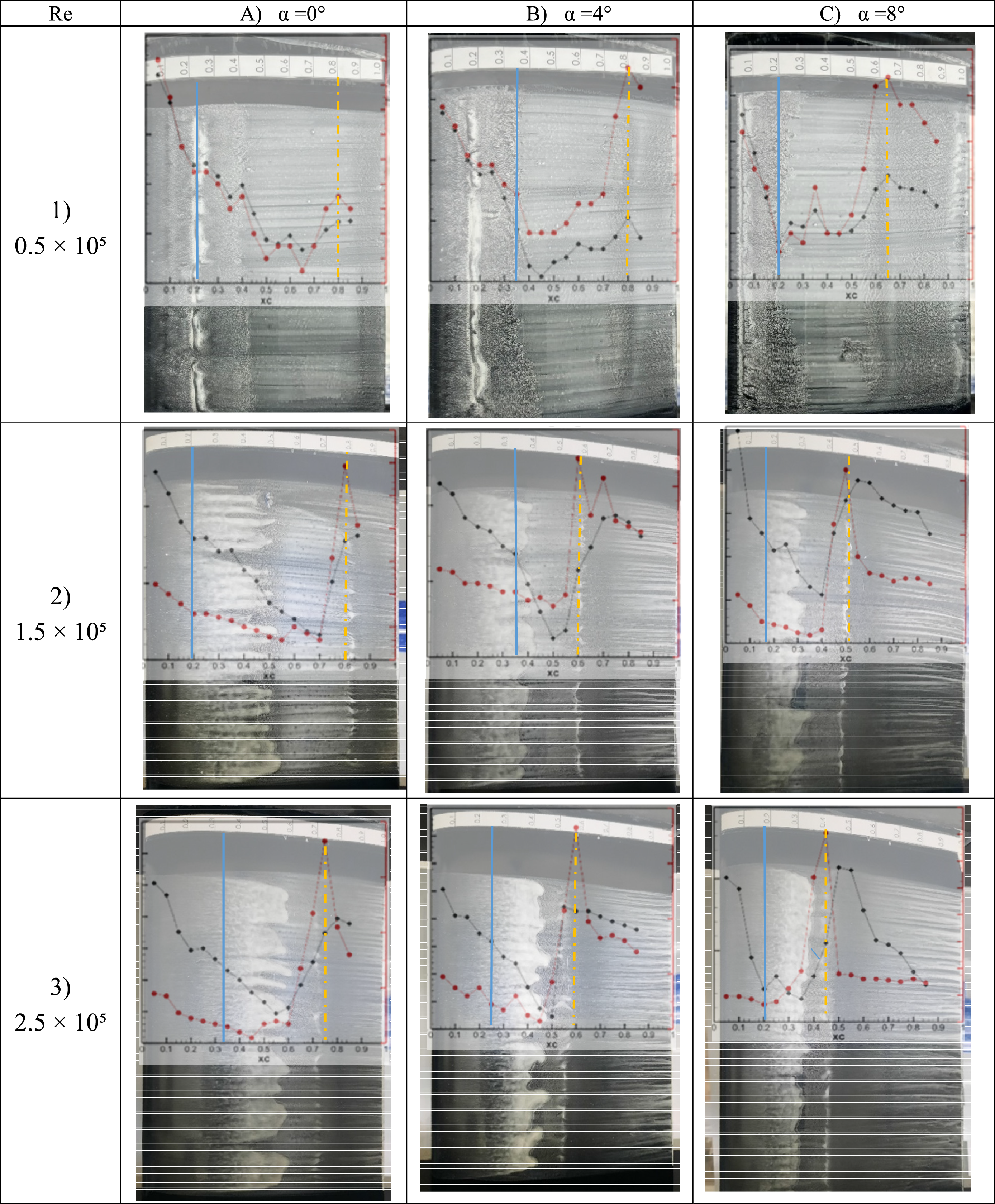
Figure 9: Comparison of oil test results with voltage (black line)-standard deviation (red line) changes at different angles of attack and Re numbers of NACA 2415 airfoil (blue line: separation point, orange line: transition point).

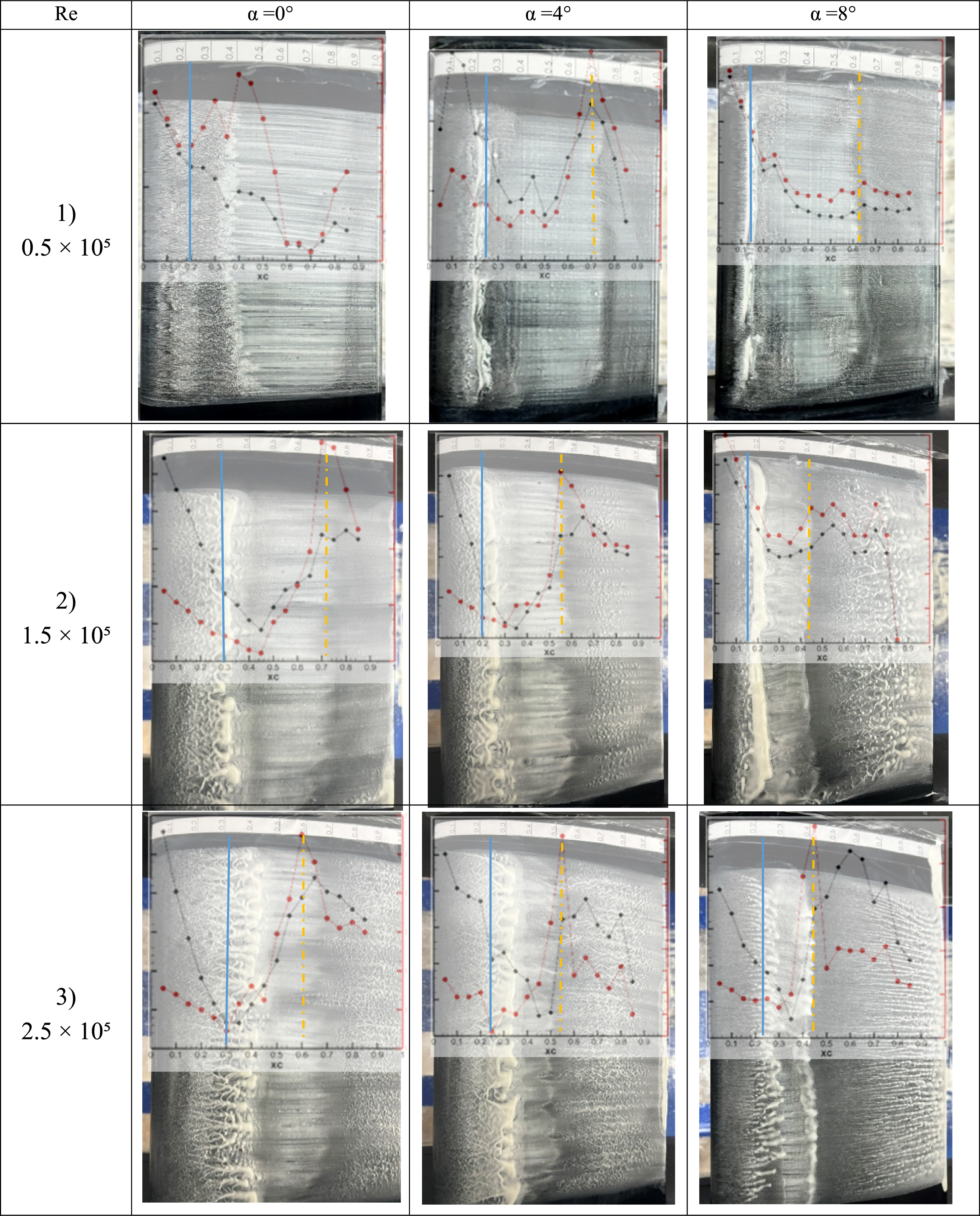
Figure 10: Comparison of oil test results with voltage (black line)-standard deviation (red line) changes at different angles of attack and Re numbers of NACA 2418 airfoil (blue line: separation point, orange line: transition point).

For the NACA 2415 airfoil at the angle of attack of 4° and Reynolds number of 0.5 × 105 (Fig. 9B1), the oil flow experiment reveals that the flow separates at x/c = 0.36, the beginning of the transition to turbulence occurs at x/c = 0.80, and subsequently reattaches to the surface. When Reynolds number is increased to 1.5 × 105 (Fig. 9B2), the flow separates slightly later at x/c = 0.38, transition is seen at x/c = 0.60, and reattaches approaching the leading edge than in the lower Reynolds number case. It is observed that the length of the separation bubble is approximately 30% of the chord length of the airfoil.

When the airfoil camber is increased from 15% to 18%, at the angle of attack of 4° and a Reynolds number of 0.5 × 105 (Figs. 9B1 and 10B1), the oil flow experiment shows that the flow separates closer to the leading edge at x/c = 0.25, transitions to turbulence at x/c = 0.70. At a Reynolds number of 1.5 × 105 (Fig. 10B2, the flow separates even closer to the leading edge at x/c = 0.20, and transition to turbulence forms at x/c = 0.55. With the effect of the change in thickness, at angles of attack of 0°, 4°, and 8°, it is observed that the location of the separation point moves from 0.12 to 0.15 (Fig. 10(C1,C2)) due to the thickness effect, and the flow separation becomes closer to the trailing edge. The point of reattachment to the surface is towards the leading edge when the thickness increases. In these two cases, the length of the bubble gets shorter. As a result, while the bubble length decreased when the thickness changed from 12% to 15%, it increased when the thickness changed from 15% to 18%.

3  Numerical Results

3.1 Pressure Distribution Results

This study examines the impact of maximum airfoil thickness on bubble formation and dynamics on the airfoil at various Reynolds numbers and angles of attack. The results obtained from the numerical modeling are presented in this section [42]. Based on the pressure distributions obtained from the numerical simulations (Fig. 11), the occurrence of bubbles can be identified through the characteristic pressure recovery regions observed along the suction side of the airfoils. At low Reynolds numbers, a distinct plateau followed by a sharp adverse pressure gradient indicates the point of boundary layer separation. In contrast, the recovery in pressure coefficients marks the subsequent reattachment [43,44]. In summary, in Cp graphs, where the change in pressure coefficient begins to resemble a straight line, a point of flow separation is pointed out. Where the straight line ends and there is a downward drop, the transition region is shown. Where there is a recovery, the reattachment point is indicated.

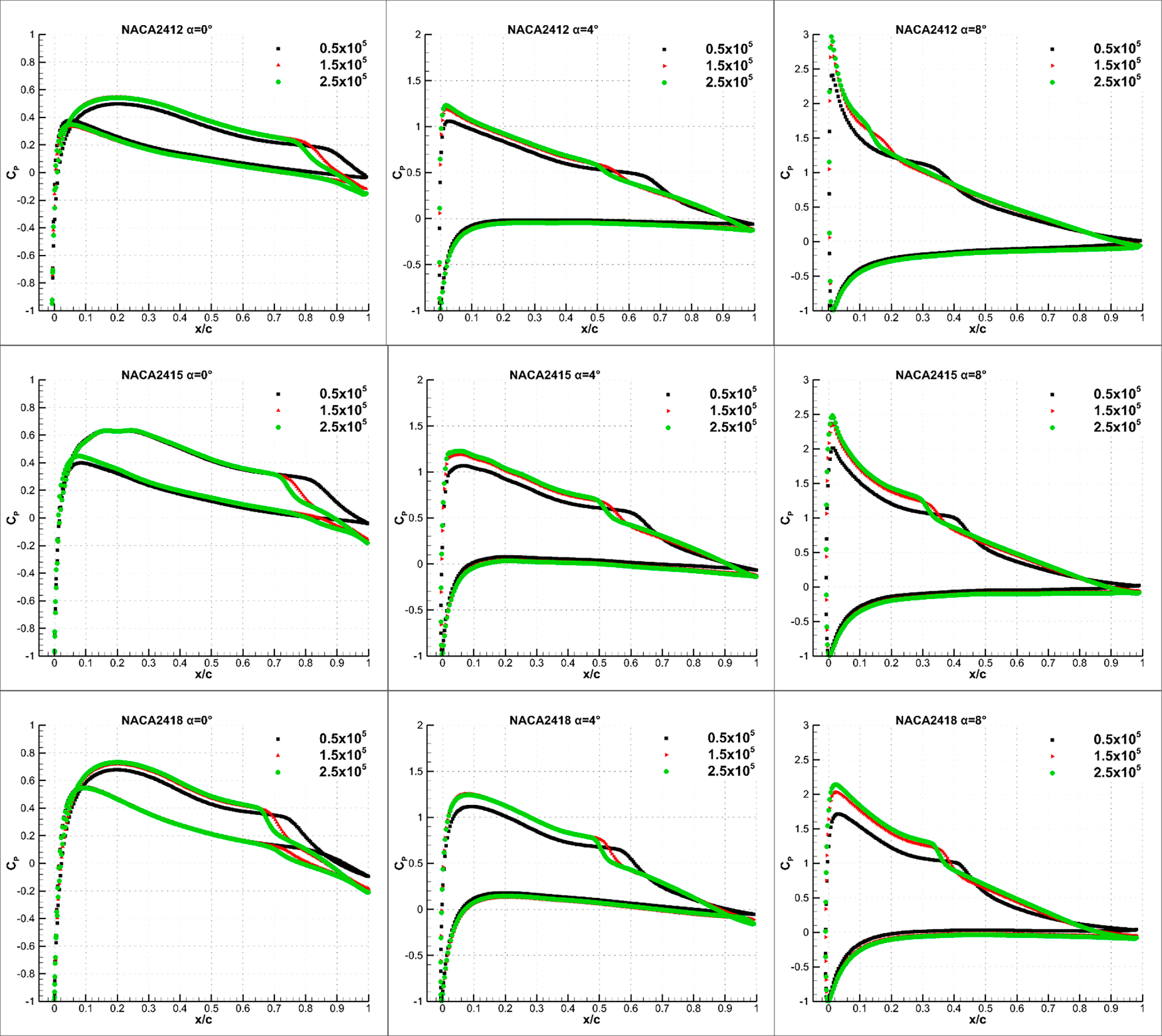
Figure 11: The pressure coefficient distribution over the airfoils obtained from numerical modeling.

According to the results obtained from the pressure distributions, at Re = 0.5 × 105 and the 0° angle of attack, the flow separation points for the NACA 2412, NACA 2415, and NACA 2418 airfoils were located at x/c = 0.59, x/c = 0.54, and x/c = 0.48, respectively. Afterwards, the flow does not reattach to the airfoil surface. For the same airfoil at the same angle of attack, with increasing Re, the flow separation points do not change significantly, but the reattachment points move toward the leading edge, and the separation bubble shortens. When the pressure distributions obtained at the 4° angle of attack are evaluated, the increasing thickness of the airfoils causes the bubble to move closer to the leading edge. For the NACA 2412 airfoil at the angle of attack of 8°, the separation points are x/c = 0.11, x/c = 0.06, and x/c = 0.05, and the reattachment points are x/c = 0.44, x/c = 0.21, and x/c = 0.14 for Re = 0.5 × 105, Re = 1.5 × 105, and Re = 2.5 × 105, respectively. The bubble length decreases from 0.33c to 0.09c. At Re = 0.5 × 105 and the 8° angle of attack, the increase in airfoil thickness causes the beginning of the bubble to move toward the trailing edge.

Overall, the results indicate that both angle of attack and Reynolds number have a significant impact on the formation and extent of laminar separation bubbles. Higher angles of attack intensify the adverse pressure gradient, enlarging the bubbles, while higher Reynolds numbers promote earlier transition, shortening their length. Furthermore, increasing the airfoil thickness from NACA 2412 to NACA 2418 systematically promotes bubble persistence, highlighting the role of geometry in the initiation and development of laminar separation bubbles. These findings highlight the delicate effects of Reynolds number and airfoil geometry on the separation-reattachment cycle that governs the aerodynamic efficiency of cambered airfoils.

3.2 Skin-Friction Coefficients Results

Analysis of the skin friction coefficient (Cf) distributions allows the quantitative determination of the separation and reattachment points in the chord direction, as well as the corresponding laminar separation bubble length. The distribution of skin friction coefficients provides information about flow separation, laminar separation bubble, and the transition to turbulence [43,44]. Flow separation occurs when the Cf coefficient value is zero for the flow over the airfoil (As sketched in Fig. 12). It then becomes negative due to a reverse flow event. If the skin friction coefficient rises above zero again, it means the flow is reattached to the airfoil surface. In conclusion, this is an important numerical result that reveals situations such as flow separations and transitions to turbulence. The results obtained from numerical modeling are presented in Fig. 12. The skin friction coefficient values show that the flow separation points for the NACA 2412, NACA 2415, and NACA 2418 airfoils are at x/c = 0.59, x/c = 0.54, and x/c = 0.48, respectively, for Re = 0.5 × 105 and the 0° angle of attack (Fig. 12). The flow does not attach to the airfoil surface after that. For the NACA 2412 airfoil, a bubble is observed at the highest Reynolds number (2.5 × 105) at α = 0°; separation occurs around x/c = 0.62, reattachment occurs at x/c = 0.81, and the LSB length is 0.19 c. At α = 4°, separation shifts upward to x/c = 0.40, and reattachment occurs at x/c = 0.52, with an LSB length of 0.12 c. At α = 8°, the separation point moves leading edge (x/c = 0.04), and reattachment occurs at x/c = 0.14, with the LSB length decreasing with increasing angle. At this angle, another LSB also forms at the trailing edge.

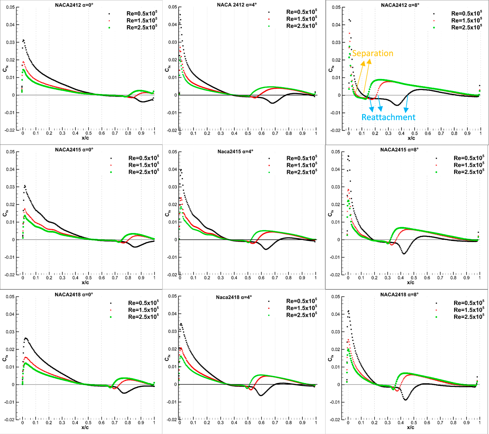
Figure 12: The skin friction coefficient distribution over the airfoils obtained from numerical modeling.

The same trend applies to the NACA 2415 airfoil. At Re = 0.5 × 105 and α = 0°, separation occurs at x/c = 0.54, and the flow cannot reattach. Increasing the angle of attack to 4° did not significantly change the flow separation. At the same Re at 8°, the separation point occurs near the leading edge (x/c = 0.19), while at x/c = 0.51, reattachment occurs, with an LSB length of 0.32c. A short bubble also forms near the trailing edge. For the thicker NACA 2418 airfoil, the separation and reattachment points are closer to the leading edge than the other two airfoils.

3.3 Streamline Results

The streamline visualisations illustrate the evolution of the flow characteristics over the airfoil surface. The streamlines obtained from the numerical modeling are given in Figs. 13–15 for three different airfoils and different flow conditions. For three different airfoils at Re = 0.5 × 105 and the angles of attack of 0°, the flow is not able to reattach after separating from the airfoil. The separation point is x/c = 0.59, x/c = 0.54 and x/c = 0.48 for the NACA2412, NACA 2415 and NACA 2418 airfoils, respectively. When the Re number is increased to 1.5 × 105 at the same angle of attack, laminar separation bubble formation is observed and the LSB length is approximately 0.26c for NACA 2412 and NACA 2415, while it is 0.24 c for NACA 2418. The increase in thickness caused a slight shortening of the LSB length. At the highest Re number of 2.5 × 105, although the bubble length is approximately 0.2 c for 3 different airfoils at the angle of attack of 0°, the initial point of the LSB moved towards the leading edge. For airfoils with three different thicknesses, increasing the Re number shortens the LSB length. The numerical modeling results indicate that in some cases, flow separation occurs again after the formation of the LSB. In some cases, after the second flow separation (for Re = 1.5 × 105 and a = 8 for NACA 2412), the flow reattaches, and LSB formation is observed, while in another case (for Re = 1.5 × 105 and α = 4° for NACA 2418), the flow cannot reattach and trailing-edge separation is observed.

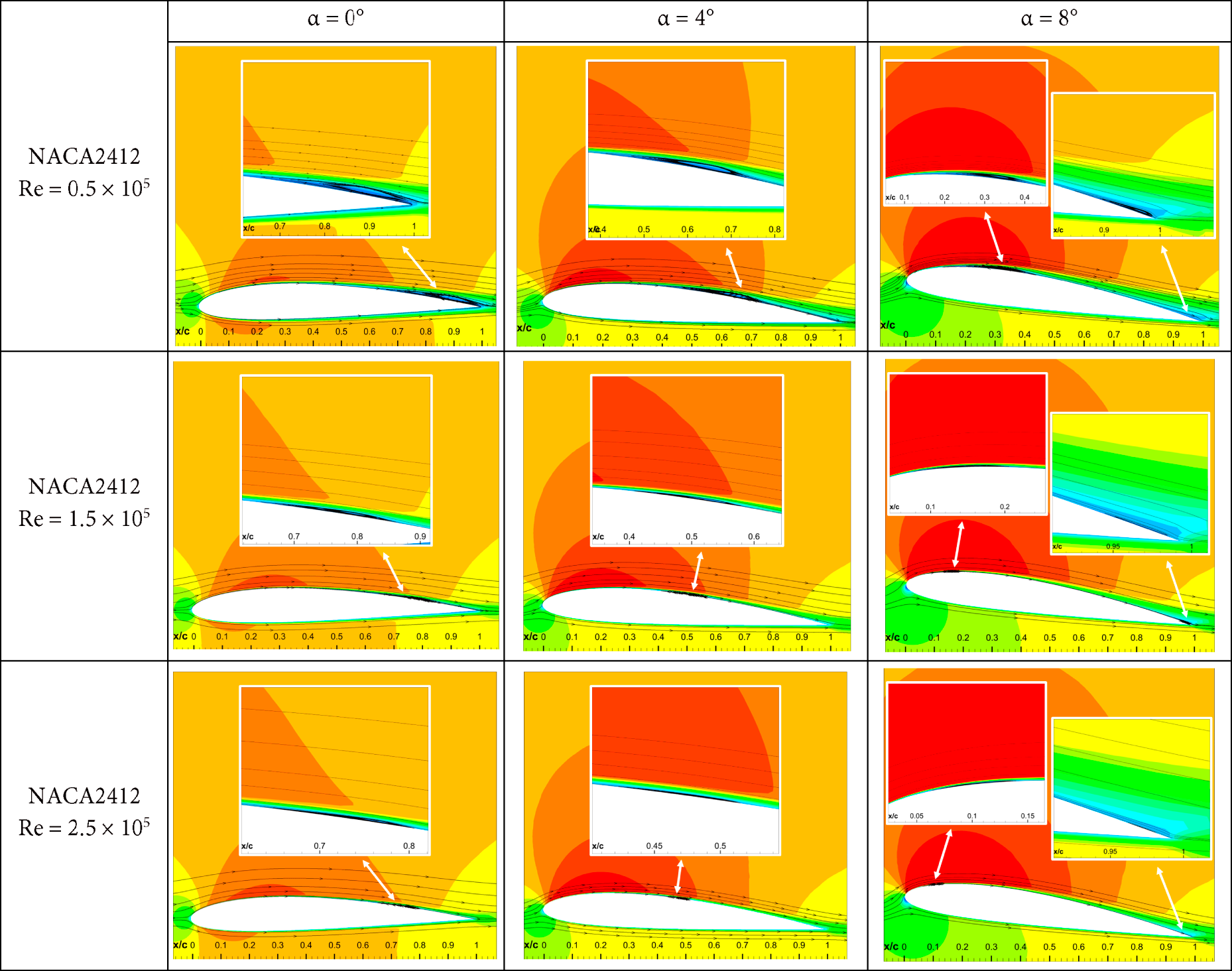
Figure 13: The streamlines for NACA2412.

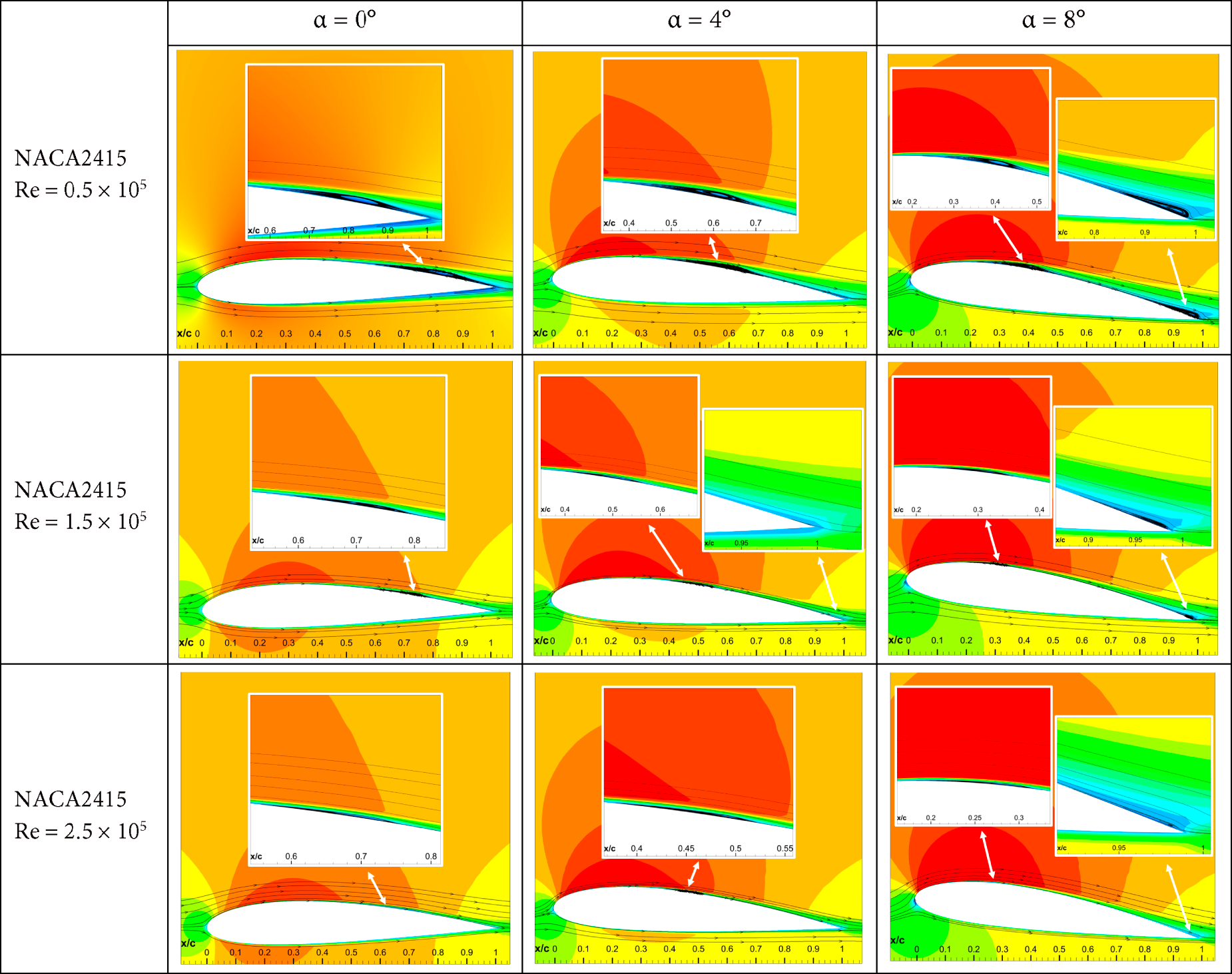
Figure 14: The streamlines for NACA2415.

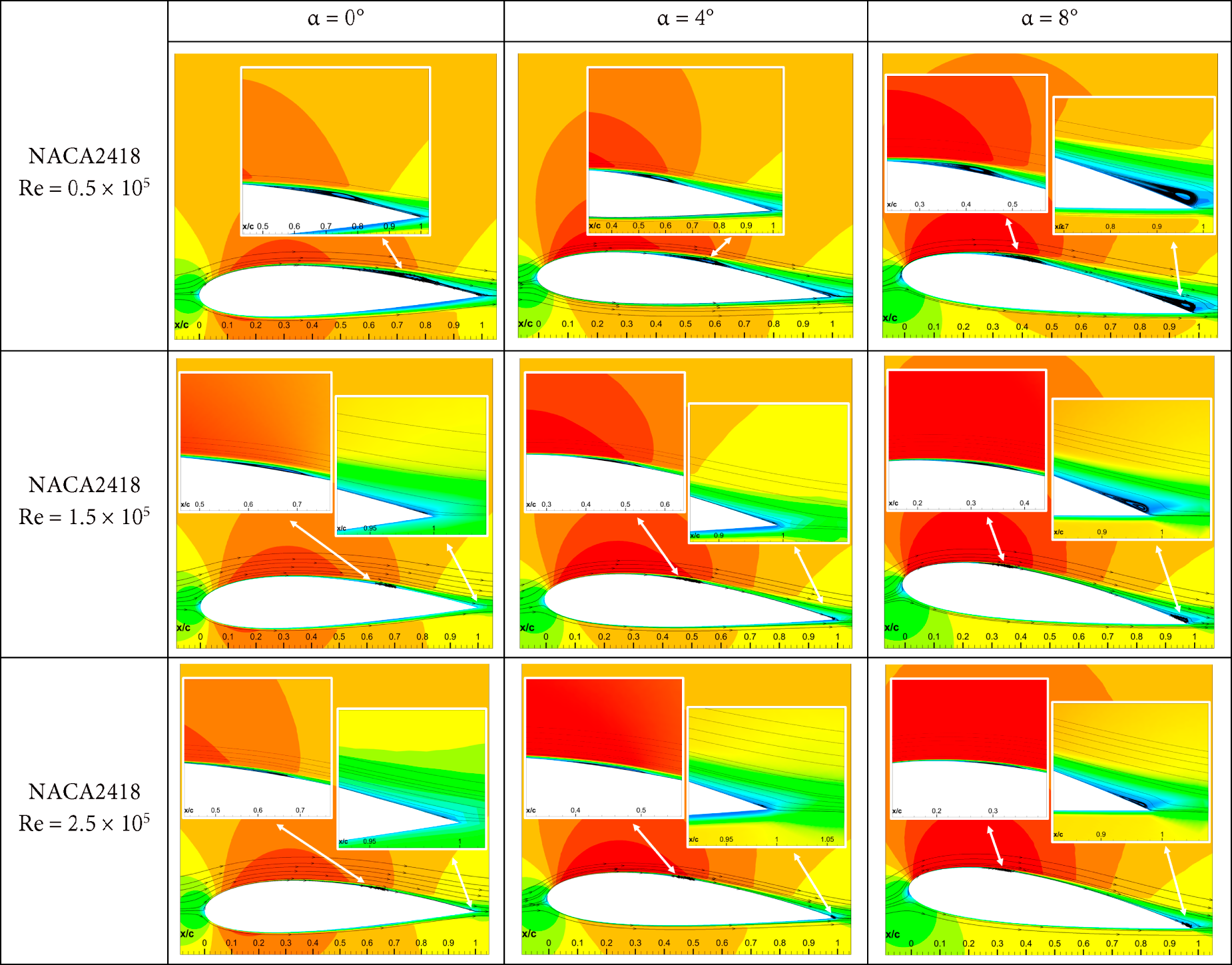
Figure 15: The streamlines for NACA2418.

3.4 Intermittency Results

The intermittency distribution predicted by ANSYS FLUENT provides insight into the laminar–turbulent transition characteristics along the surface. This parameter varies between 0 and 1; values close to zero indicate a fully laminar boundary layer, while values close to 1 correspond to a fully turbulent state. Intermediate values describe the transitional regime, in which patches of laminar and turbulent flow appear alternately. The intermittency distributions of the numerical modeling performed at different angles of attack and Re numbers are presented in Figs. 16–18 for NACA 2412, NACA 2415 and NACA 2418, respectively. The intermittency results for NACA 2412 are given in Fig. 16. When the results for Re = 0.5 × 105 are examined for a = 0°, it is observed that the intermittency values decrease after the trailing edge of the airfoil as the Re number increases. Fig. 17 shows the intermittency values obtained from numerical modeling for NACA 2415. Comparing Figs. 16 and 17, it can be seen that increasing the thickness of the wing causes the formation of the separation bubble to approach the leading edge. When the intermittency values obtained from numerical modeling are examined for 3 different airfoils, it is understood that for Re = 0.5 × 105, as the angle of attack increases, the intermittency values that provide information about the transition to turbulence approach the leading edge and the transition to turbulence begins earlier. When the intermittency results for NACA2415 in Fig. 17 are evaluated for Re = 2.5 × 105, it is seen that the intermittency values increase after the trailing edge with the increase in the angle of attack. For the airfoil with the highest thickness, increasing the Re number led to a decrease in the thickness of the laminar boundary layer (Fig. 18).

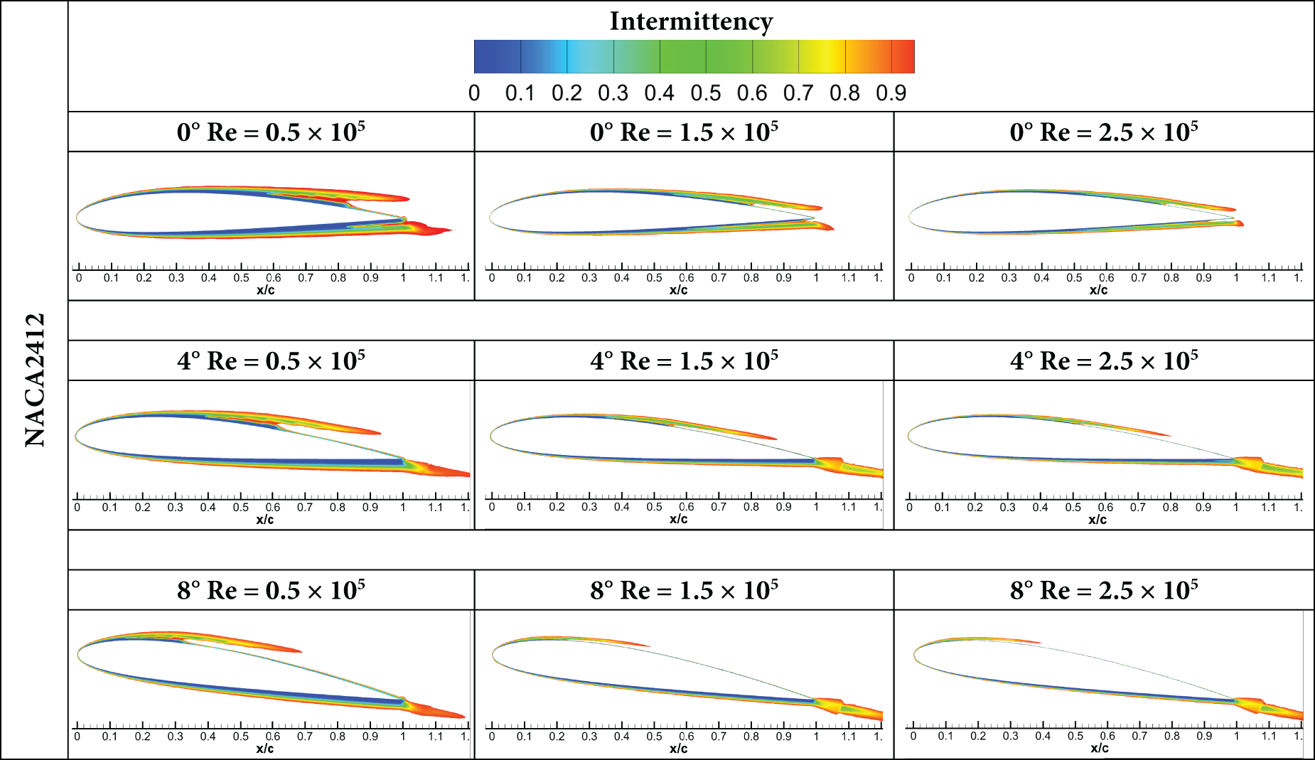
Figure 16: The intermittency results for NACA2412.

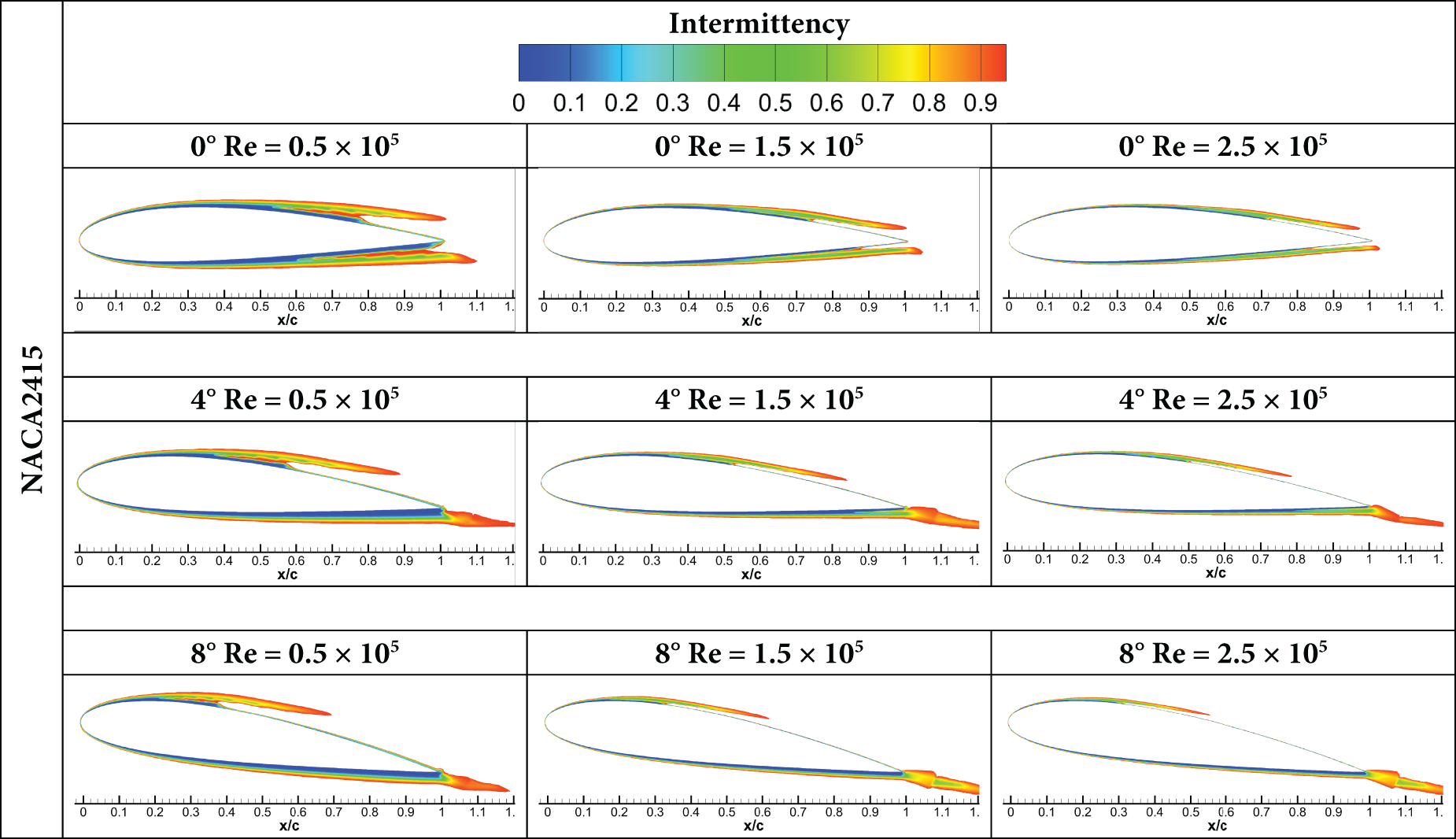
Figure 17: The intermittency results for NACA2415.

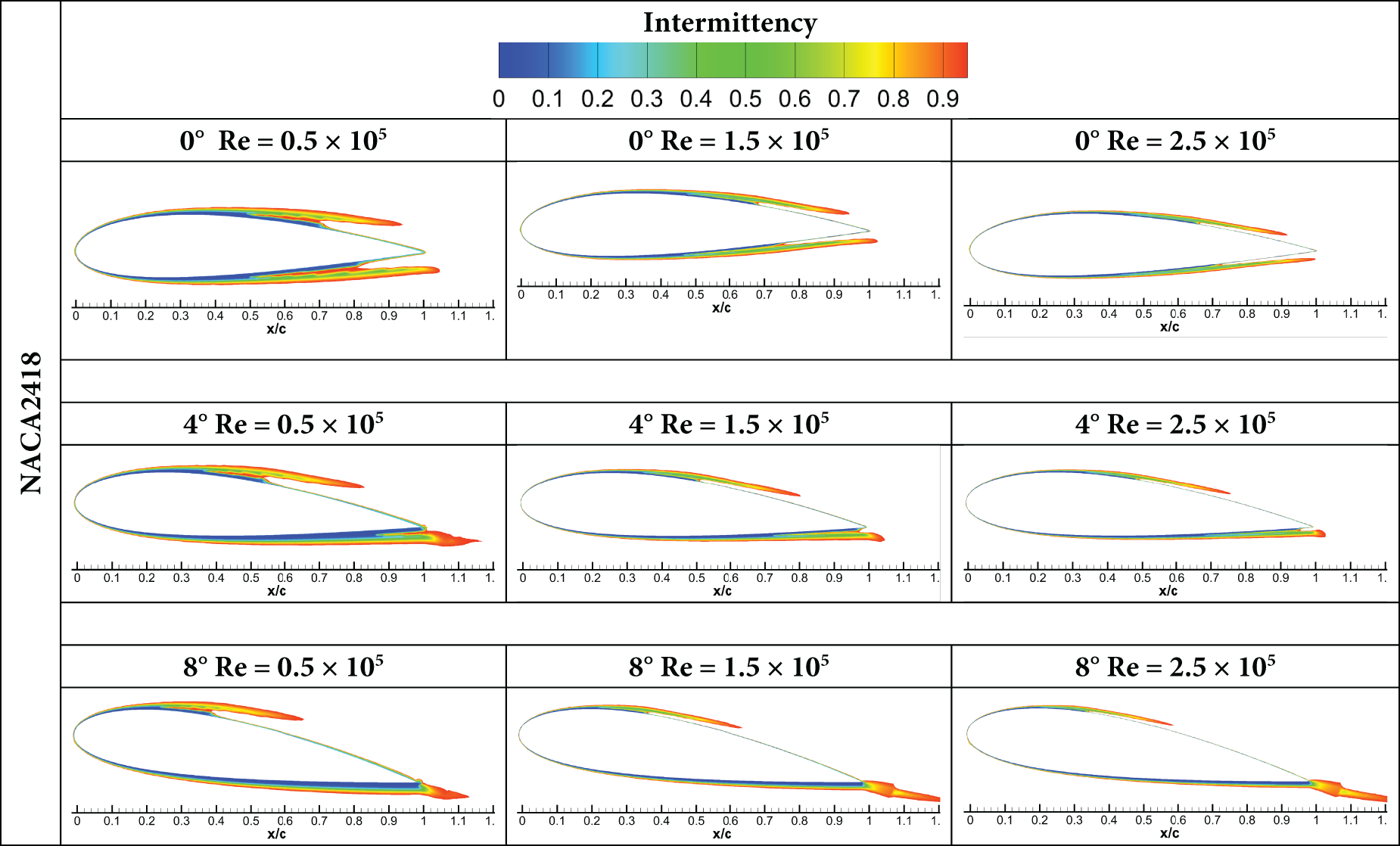
Figure 18: The intermittency results for NACA2418.

3.5 Turbulence Kinetic Energy Results

The turbulence kinetic energy (TKE) predicted in ANSYS FLUENT serves as a fundamental indicator of the intensity of turbulent fluctuations within the flow field. TKE represents the mean kinetic energy per unit mass (J/kg = m2 s−2) associated with velocity fluctuations, and its magnitude provides a direct measure of turbulence strength. Elevated values of TKE are typically observed in regions of strong shear, near-wall boundary layers, flow separation zones, and wake regions. In contrast, low values correspond to laminar or weakly disturbed flow. The spatial distribution of TKE is beneficial for identifying the onset and development of turbulence. A rapid increase in TKE downstream of transition onset indicates the amplification of instabilities and the breakdown of laminar flow structures. Furthermore, the extent and peak levels of TKE highlight areas of high momentum exchange and energy dissipation, which directly influence aerodynamic performance, mixing characteristics, and boundary-layer stability.

In this study, the TKE distributions obtained from modeling are given in Figs. 19 and 20. When the obtained results are examined, the results are given according to the change in Re number for a more understandable comparison of the TKE values. When Fig. 19 is evaluated (for Re = 0.5 × 105), it is seen that for airfoils with the same thickness, high TKE values approach the leading edge with increasing angle of attack. Fig. 20 presents the results obtained for Re = 1.5 × 105. The increase in the Reynolds number causes the TKE values in the flow region on the upper surface of the airfoil to increase. When the results obtained for Re = 2.5 × 105 are evaluated, it is observed that an increase in airfoil thickness at the same angle of attack leads to higher TKE values and stronger turbulence in the wake region behind the airfoil (Fig. 21).

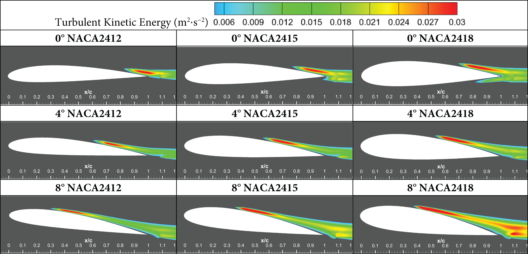
Figure 19: The TKE results of the airfoils at Re = 0.5 × 105.

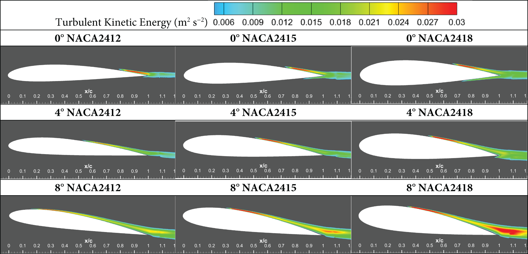
Figure 20: The TKE results of the airfoils at Re = 1.5 × 105.

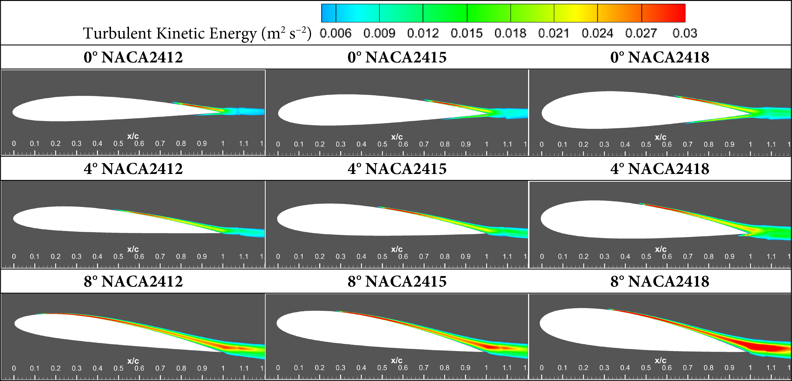
Figure 21: The TKE results of the airfoils at Re = 2.5 × 105.

3.6 Modeling of the Bubble with Modified Parameters

While experimental investigation of flow characteristics over an airfoil surface provides more consistent and accurate results [41], numerical methods represent a package of various derived and non-derived parameters as an output. From that point, a numerical study is also performed in order to compare how separation and reattachment points differ in each method [42]. As experimental methods were already explained in previous sections, a discussion of how numerical approaches and input parameters affect the solution is crucial. A four-equation RANS model, Transition-SST is used to determine flow separation and reattachment. It basically consists of a turbulence kinetic energy term k, a specific dissipation rate term ω, an intermittency term γ, and Reθt term which directly affects the onset of transition. Furthermore, by modifying this parameter it is possible to obtain a more accurate transition onset since it represents the transition onset momentum thickness Reynolds number. The idea behind these modifications is correctly adjusting the relation between Reθt and some flow characteristics such as turbulence intensity, adverse pressure gradient. If a correctly calculated Reθt value is entered as the input condition, the transition onset point can also be correctly determined. The relationship that ensures this is the direct effect of the value given as the inlet condition on the local value, and the local value itself being the leading parameter in one of the four main equations used in the transition model. Another influential parameter that needs to be considered is the critical Reynolds number, Reθc, which depends on the momentum thickness at which the first signs of transition to turbulence appear. The location here is generally considered to be the place where the intermittency value makes an unusual rise for the first time. Similarly, this value directly affects the transition start. It’s fair to say that these two parameters represent two dimensionless distances along streamwise. It is important to note that the Reθc value should always be smaller than the Reθt value, because the first traces of the transition are seen in the intermittency values. In this study, Reθt and Reθt values were recalculated based on various airfoil and flow characteristics, including thickness, camber, Re-number, and angle of attack, as well as data on boundary layer characteristics obtained from experimental studies. These recalculated values were then converted into input data in FLUENT using a User-Defined Function (UDF). In the graph shown in Fig. 22, the X-wall shear stress graph shows several cases where the Transition-SST model is used. One of these is the default case, which means no input conditions are given on these parameters. In Fig. 22, when different inlet conditions are applied to the Reθt and Reθc, the flow separation, transition onset, and reattachment positions change. The difference is particularly pronounced between the locations where the curve transitions from negative to positive, indicating flow reattachment. In Fig. 23, two specific situations are examined in more detail. Similarly, in Fig. 23, when the velocity contours and streamlines of the default case on the left and a randomly selected modified case on the right are considered, there is a change in the structure of the laminar separation bubble and the start-end positions indicating the separation-reattachment points. In Fig. 24, a comparison with experimental results is given and in particular, it is revealed how the modified numerical situations can approach the experimental results.

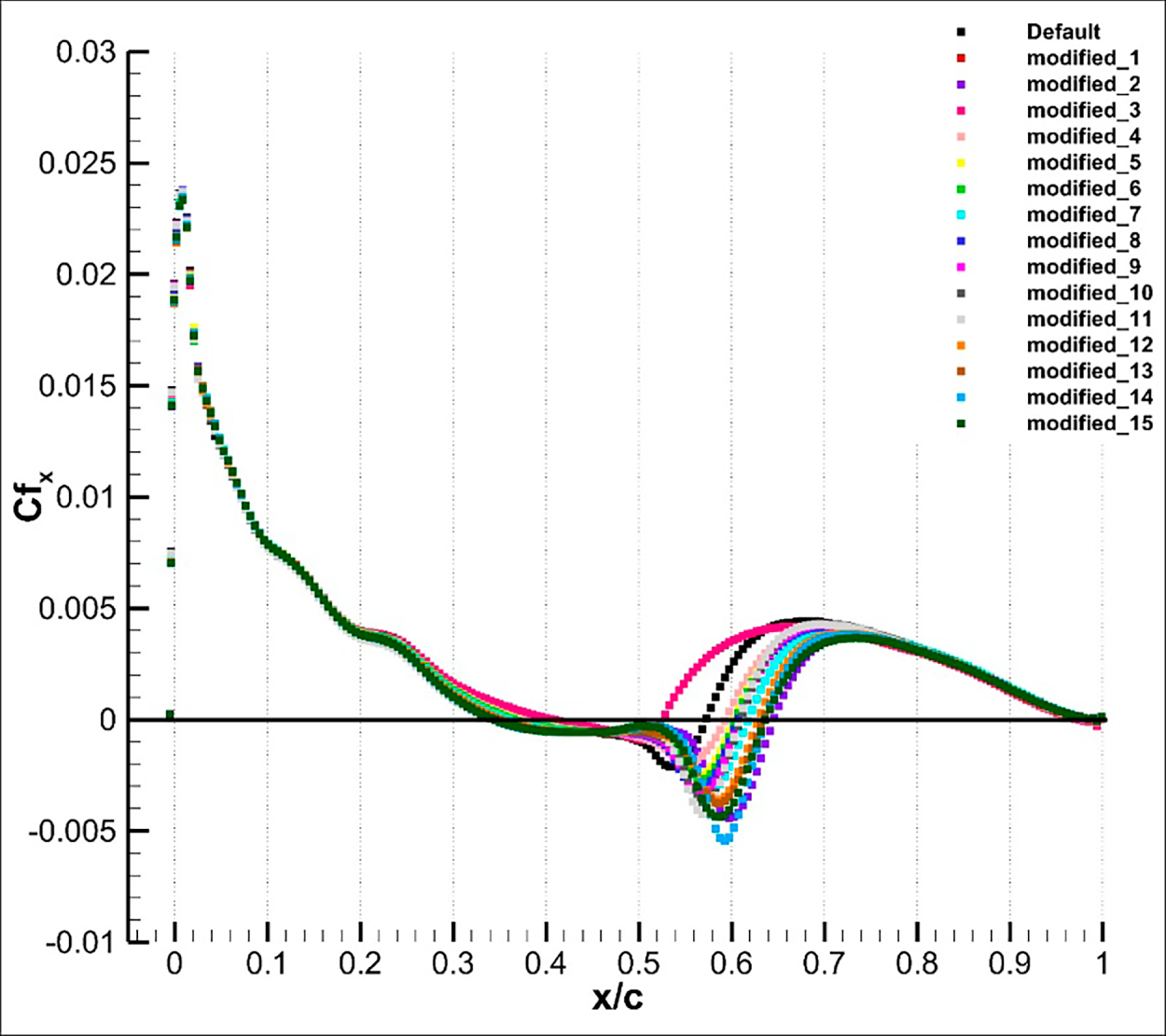
Figure 22: Default case and modified cases representing different for NACA2415 at Re = 1.5 × 105 and α = 4°.

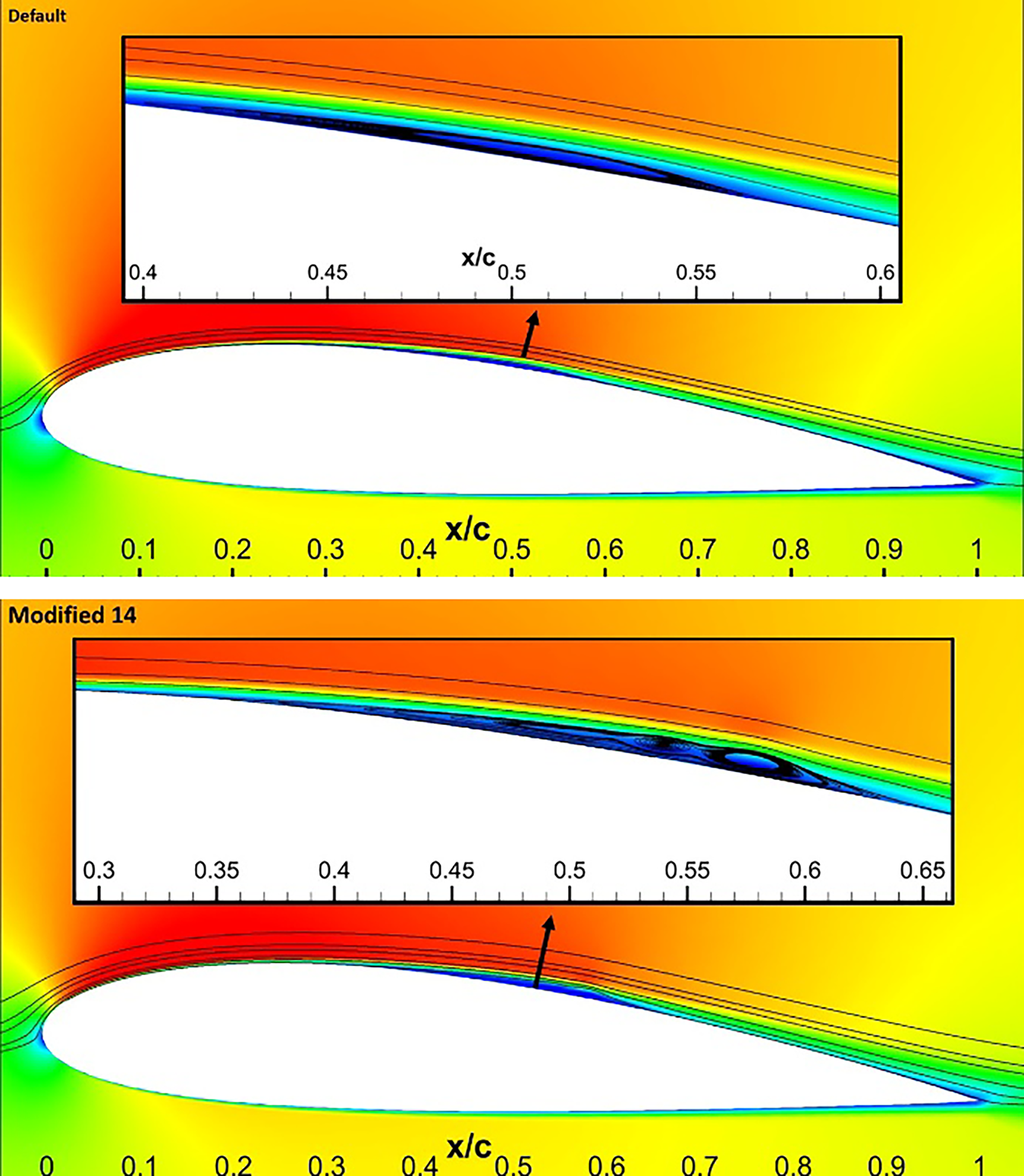
Figure 23: Velocity contours and streamlines for the default case and a specifically selected case.

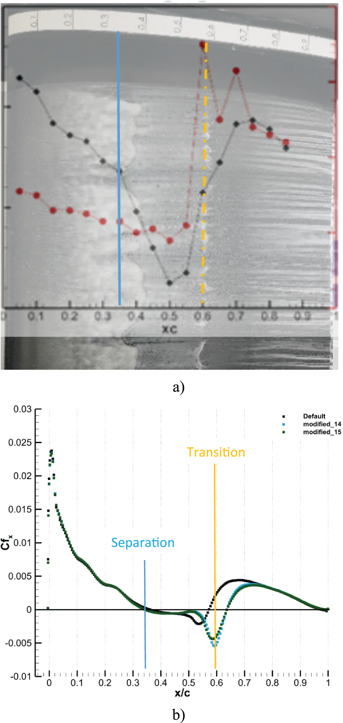
Figure 24: Comparison of (a) the experimental result [41] with (b) the default and modified numerical result [42] for NACA2415 at Re = 1.5 × 105 and α = 4°.

When examining the oil flow visualization and hot-film sensor experiments in Fig. 24, the separation and reattachment points are approximately at x/c = 0.35 and 0.67, respectively. Conversely, in the default numerical solution, the separation point is very close to the experimental result, while reattachment occurs around x/c = 0.57. On the other hand, while there is no significant difference in the separation point in the modified numerical result compared to the experimental and default numerical results, the reattachment point is very close to the experimental situation, around 0.64. This emerging scenario demonstrates the direct impact of different initial conditions for the Reθt and Reθc parameters on the transition onset position. The closer reattachment result also confirms that the transition onset occurs after separation has already occurred, before reattachment, in a region above the laminar separation bubble.

4  Conclusion

In this study, LSB formation for airfoils with different thicknesses is investigated in detail numerically and experimentally. The variation in Reynolds number and angle of attack, as well as the thickness variation, for airfoils with the same thickness, is evaluated in detail in terms of LSB formation regions. For the lowest Re number in the study (Re = 0.5 × 105), increasing the airfoil thickness at the angle of attack of 0° caused the flow separation point to move towards the leading edge from x/c = 0.59 to x/c = 0.48. According to the numerical findings, increasing the Reynolds number and airfoil thickness results in higher TKE values, an earlier onset of transition and turbulence, and stronger turbulent activity, particularly in the upper surface flow and wake regions. Overall, the presence and extent of the laminar separation bubble are strongly influenced by the Reynolds number, angle of attack, and airfoil geometry. These bubbles can significantly affect airfoil performance, increase drag, and alter lift behavior at low Reynolds numbers.

The reattachment point is quite near to the experimental scenario, but the separation point in the adjusted numerical result is not significantly different from the experimental and default numerical findings. This emergent scenario shows how the transition start position is directly affected by various initial conditions for the momentum thickness parameters. Additionally, the closer reattachment finding verifies that the transition commencement takes place at an area above the laminar separation bubble after separation has already taken place, before reattachment.

This study demonstrates that the newly developed turbulent transition model for modeling separation bubbles still has shortcomings and needs to be improved by updating empirical equations and parameters, supported by more experimental data. Moreover, integration of airfoil and flow characteristics into the equations in bubble modeling is an important point for future studies.

Acknowledgement: The authors are grateful to the Scientific and Technological Research Council of Turkey (TÜBİTAK) for support, and to the Scientific Research Projects Unit of Erciyes University.

Funding Statement: The authors are grateful to the Scientific and Technological Research Council of Turkey (TÜBİTAK) for support under project number: 122M826; and to the Scientific Research Projects Unit of Erciyes University under contract No.: FYL-2023-13162 and FYL-2024-13701.

Author Contributions: The authors confirm contribution to the paper as follows: Conceptualization: Mustafa Serdar Genç, Mustafa Özden, Halil Hakan Açıkel; methodology: Mustafa Serdar Genç, Halil Hakan Açıkel, Eren Anıl Sezer, Muhammer Ayvazoğlu, Muhammed Hatem; software: Mustafa Özden, Eren Anıl Sezer, Muhammed Hatem; validation: Eren Anıl Sezer, Muhammer Ayvazoğlu, Sinem Keskin, Muhammed Hatem; formal analysis: Eren Anıl Sezer, Muhammer Ayvazoğlu, Sinem Keskin, Muhammed Hatem, Mustafa Özden; investigation: Eren Anıl Sezer, Muhammer Ayvazoğlu, Sinem Keskin, Muhammed Hatem; data curation: Eren Anıl Sezer, Muhammer Ayvazoğlu, Mustafa Özden, Muhammed Hatem; writing—original draft preparation: Mustafa Serdar Genç, Halil Hakan Açıkel; writing—review and editing: Mustafa Serdar Genç, Halil Hakan Açıkel; visualization: Eren Anıl Sezer, Muhammer Ayvazoğlu, Mustafa Serdar Genç, Mustafa Özden, Sinem Keskin, Muhammed Hatem; supervision: Mustafa Serdar Genç, Halil Hakan Açıkel; project administration: Mustafa Serdar Genç, Halil Hakan Açıkel; funding acquisition: Mustafa Serdar Genç, Halil Hakan Açıkel. All authors reviewed and approved the final version of the manuscript.

Availability of Data and Materials: The data that support the findings of this study are available from the corresponding author, Mustafa Serdar Genç, upon reasonable request.

Ethics Approval: Not applicable.

Conflicts of Interest: The authors declare no conflicts of interest.

References

1. Gaster M. The structure and behaviour of separation bubbles. Cranfield, UK: Cranfield University; 1967. [Google Scholar]

2. Horton HP. Laminar separation bubbles in two and three dimensional incompressible flow [dissertation]. London, UK: Queen Mary University of London; 1968. [Google Scholar]

3. Roberts WB. Calculation of laminar separation bubbles and their effect on airfoil performance. AIAA J. 1980;18(1):25–31. doi:10.2514/3.50726. [Google Scholar] [CrossRef]

4. Castiglioni G, Domaradzki JA, Pasquariello V, Hickel S, Grilli M. Numerical simulations of separated flows at moderate Reynolds numbers appropriate for turbine blades and unmanned aero vehicles. Int J Heat Fluid Flow. 2014;49:91–9. doi:10.1016/j.ijheatfluidflow.2014.02.003. [Google Scholar] [CrossRef]

5. Hain R, Kähler CJ, Radespiel R. Dynamics of laminar separation bubbles at low-Reynolds-number aerofoils. J Fluid Mech. 2009;630:129–53. doi:10.1017/s0022112009006661. [Google Scholar] [CrossRef]

6. Zhang W, Cheng W, Gao W, Qamar A, Samtaney R. Geometrical effects on the airfoil flow separation and transition. Comput Fluids. 2015;116:60–73. doi:10.1016/j.compfluid.2015.04.014. [Google Scholar] [CrossRef]

7. Ayvazoğlu M, Keskin S, Şahin R, Sincar M, Sezer EA, Açıkel HH, Özden M, Genç MS. Numerical and experimental investigation of thickness effect on the cambered airfoils at low reynolds numbers. J Aeronaut Space Technol. 2024;17:116–34. [Google Scholar]

8. Giacomini E, Westerberg LG. CFD analysis of transition models for low-Reynolds number aerodynamics. Appl Sci. 2025;15(18):10299. doi:10.3390/app151810299. [Google Scholar] [CrossRef]

9. Matsson JE, Voth JA, McCain CA, McGraw C. Aerodynamic performance of the NACA, 2412 airfoil at Low Reynolds Number. In: Proceedings of the 2016 ASEE Annual Conference & Exposition; 2016 Jun 26–29; New Orlean, LA, USA. [Google Scholar]

10. Carreño Ruiz M, D’Ambrosio D. Validation of the γ-Reθ transition model for airfoils operating in the very low Reynolds number regime. Flow Turbul Combust. 2022;109(2):279–308. doi:10.1007/s10494-022-00331-z. [Google Scholar] [CrossRef]

11. Liu Y, Li P, Jiang K. Comparative assessment of transitional turbulence models for airfoil aerodynamics in the low Reynolds number range. J Wind Eng Ind Aerodyn. 2021;217:104726. doi:10.1016/j.jweia.2021.104726. [Google Scholar] [CrossRef]

12. Michna J, Rogowski K. Numerical study of the effect of the Reynolds number and the turbulence intensity on the performance of the NACA 0018 airfoil at the low Reynolds number regime. Processes. 2022;10(5):1004. doi:10.3390/pr10051004. [Google Scholar] [CrossRef]

13. Klose BF, Spedding GR, Jacobs GB. Direct numerical simulation of cambered airfoil aerodynamics at Re = 20,000. arXiv:2108.04910. 2021. [Google Scholar]

14. Michna J, Śledziewski M, Rogowski K. The harmonic pitching NACA, 0018 airfoil in low Reynolds number flow. Energies. 2025;18(11):2884. doi:10.3390/en18112884. [Google Scholar] [CrossRef]

15. Tanürün HE, Akın AG, Acır A, Şahin İ. Experimental and numerical investigation of roughness structure in wind turbine airfoil at low Reynolds number. Int J Thermodyn. 2024;27(3):26–36. doi:10.5541/ijot.1455513. [Google Scholar] [CrossRef]

16. Tangermann E, Klein M. Numerical simulation of laminar separation on a NACA0018 airfoil in freestream turbulence. In: AIAA Scitech 2020 Forum. Orlando, FL, USA: AIAA; 2020. p. 2020–64. doi:10.2514/6.2020-2064. [Google Scholar] [CrossRef]

17. Roberts WB. The effect of Reynolds number and laminar separation on axial cascade performance. J Eng Power. 1975;97(2):261–73. doi:10.1115/1.3445978. [Google Scholar] [CrossRef]

18. McAuliffe BR, Yaras MI. Transition mechanisms in separation bubbles under low- and elevated-freestream turbulence. J Turbomach. 2010;132:011004. doi:10.1115/1.2812949. [Google Scholar] [CrossRef]

19. Dellacasagrande M, Lengani D, Simoni D, Yarusevych S. A data-driven analysis of short and long laminar separation bubbles. J Fluid Mech. 2023;976:R3. doi:10.1017/jfm.2023.960. [Google Scholar] [CrossRef]

20. Jaroslawski T, Forte M, Vermeersch O, Moschetta JM, Gowree ER. Disturbance growth in a laminar separation bubble subjected to free-stream turbulence. J Fluid Mech. 2023;956:A33. doi:10.1017/jfm.2023.23. [Google Scholar] [CrossRef]

21. Samson A, Sarkar S. Effects of free-stream turbulence on transition of a separated boundary layer over the leading-edge of a constant thickness airfoil. J Fluids Eng. 2016;138(2):021202. doi:10.1115/1.4031249. [Google Scholar] [CrossRef]

22. Kumar R, Sarkar S. Features of laminar separation bubble subjected to varying adverse pressure gradients. Phys Fluids. 2023;35(12):124104. doi:10.1063/5.0177593. [Google Scholar] [CrossRef]

23. Açıkel HH, Genç MS. Control of laminar separation bubble over wind turbine airfoil using partial flexibility on suction surface. Energy. 2018;165:176–90. doi:10.1016/j.energy.2018.09.040. [Google Scholar] [CrossRef]

24. Boutilier MSH, Yarusevych S. Separated shear layer transition over an airfoil at a low Reynolds number. Phys Fluids. 2012;24(8):084105. doi:10.1063/1.4744989. [Google Scholar] [CrossRef]

25. Alam M, Sandham ND. Direct numerical simulation of ‘short’ laminar separation bubbles with turbulent reattachment. J Fluid Mech. 2000;410:1–28. doi:10.1017/s0022112099008976. [Google Scholar] [CrossRef]

26. Howard RJA, Alam M, Sandham ND. Two-equation turbulence modelling of a transitional separation bubble. Flow Turbul Combust. 2000;63(1):175–91. doi:10.1023/A:1009992406036. [Google Scholar] [CrossRef]

27. Rumsey CL, Spalart PR. Turbulence model behavior in low Reynolds number regions of aerodynamic flowfields. AIAA J. 2009;47(4):982–93. doi:10.2514/1.39947. [Google Scholar] [CrossRef]

28. Catalano P, Tognaccini R. Turbulence modeling for low-Reynolds-number flows. AIAA J. 2010;48(8):1673–85. doi:10.2514/1.j050067. [Google Scholar] [CrossRef]

29. Menter FR, Esch T, Kubacki S. Transition modelling based on local variables. In: Engineering turbulence modelling and experiments 5. Amsterdam, The Netherlands: Elsevier; 2002. p. 555–64. doi:10.1016/b978-008044114-6/50053-3. [Google Scholar] [CrossRef]

30. Abraham JP, Sparrow EM, Gorman JM, Zhao Y, Minkowycz WJ. Application of an intermittency model for laminar, transitional, and turbulent internal flows. J Fluids Eng. 2019;141(7):0712041–8. doi:10.1115/1.4042664. [Google Scholar] [PubMed] [CrossRef]

31. Mayle RE. The role of laminar-turbulent transition in gas turbine engines. In: Proceedings of the ASME 1991 International Gas Turbine and Aeroengine Congress and Exposition; 1991 Jun 3–6; Orlando, FL, USA. doi:10.1115/91-GT-261. [Google Scholar] [CrossRef]

32. Gostelow JP, Blunden AR, Walker GJ. Effects of free-stream turbulence and adverse pressure gradients on boundary layer transition. J Turbomach. 1994;116(3):392–404. doi:10.1115/1.2929426. [Google Scholar] [CrossRef]

33. Steelant J, Dick E. Modelling of bypass transition with conditioned navier-stokes equations coupled to an intermittency transport equation. Int J Numer Meth Fluids. 1996;23(3):193–220. doi:10.1002/(SICI)1097-0363(19960815)23:. [Google Scholar] [CrossRef]

34. Suzen Y, Huang P. An intermittency transport equation for modeling flow transition. In: 38th Aerospace Sciences Meeting and Exhibit. Reno, NV, USA: AIAA; 2000. p. 2000–287. doi:10.2514/6.2000-287. [Google Scholar] [CrossRef]

35. Menter FR, Langtry RB, Likki SR, Suzen YB, Huang PG, Völker S. A correlation-based transition model using local variables: part I: model formulation. J Turbomach. 2006;128(3):413. doi:10.1115/1.2184352. [Google Scholar] [CrossRef]

36. Sekhoune Özden K, Karasu İ, Genç MS. Experimental investigation of the ground effect on a wing without/with trailing edge flap. Fluid Dyn Res. 2020;52(4):045504. doi:10.1088/1873-7005/aba1d8. [Google Scholar] [CrossRef]

37. Karasu I, Genc MS, Açıkel HH, Akpolat MT. An experimental study on laminar separation bubble and transition over an aerofoil at low Reynolds number. In: Proceedings of the 30th AIAA Applied Aerodynamics Conference; 2012 Jun 25–28; New Orleans, LA, USA. doi:10.2514/6.2012-3030. [Google Scholar] [CrossRef]

38. Karasu I, Sahin B, Tasci MO, Akilli H. Effect of yaw angles on aerodynamics of a slender delta wing. J Aerosp Eng. 2019;32(5):04019074. doi:10.1061/(asce)as.1943-5525.0001066. [Google Scholar] [CrossRef]

39. Algan M, Seyhan M, Sarioğlu M. Effect of aero-shaped vortex generators on NACA, 4415 airfoil. Ocean Eng. 2024;291:116482. doi:10.1016/j.oceaneng.2023.116482. [Google Scholar] [CrossRef]

40. Zhang X, Mahallati A, Sjolander S. Hot-film measurements of boundary layer transition, separartion and reattachment on a low-pressure turbine airfoil at low Reynolds numbers. In: Proceedings of the 38th AIAA/ASME/SAE/ASEE Joint Propulsion Conference & Exhibit; 2002 Jul 7–10; Indianapolis, IN, USA. doi:10.2514/6.2002-3643. [Google Scholar] [CrossRef]

41. Ayvazoğlu M. Investigation of the effect of thickness on the formation of laminar separation bubble on different cambered airfoils at low Reynolds number flows [master’s thesis]. Kayseri, Türkiye: Erciyes University; 2024. [Google Scholar]

42. Sezer EA. Modelling of the laminar separation bubble formed on various airfoils using different parameters [master’s thesis]. Kayseri, Türkiye: Erciyes University; 2026. [Google Scholar]

43. Genç M, Kaynak Ü. Control of flow separation and transition point over an aerofoil at low Re number using simultaneous blowing and suction. In: Proceedings of the 19th AIAA Computational Fluid Dynamics; 2009 Jun 22–25; San Antonio, TX, USA. doi:10.2514/6.2009-3672. [Google Scholar] [CrossRef]

44. Genç MS, Karasu I, Açıkel HH, Akpolat MT. Low Reynolds number flows and transition. In: Genç M, editor. Low Reynolds number aerodynamics and transition. London, UK: IntechOpen; 2012. p. 3–28. doi:10.5772/31131. [Google Scholar] [CrossRef]