
 Login
Login Register
 Submit a Paper
 Propose a Special lssue
 Open Access
ARTICLE

A Comparative Study of State-of-the-Art Meshless Methods for Flow and Transport Simulation in Porous Media
1 Department of Civil Engineering, Indian Institute of Technology Bombay, Mumbai, Maharashtra, India
2 Department of Civil Engineering, School of Infrastructure, Indian Institute of Technology Bhubaneswar Argul, Khordha, Odisha, India
3 Department of Environmental Science and Engineering, Indian Institute of Technology (Indian School of Mines), Dhanbad, Jharkhand, India
* Corresponding Author: T. I. Eldho. Email:
Computer Modeling in Engineering & Sciences 2026, 147(2), 26 https://doi.org/10.32604/cmes.2026.078705
Received 06 January 2026; Accepted 15 April 2026; Issue published 27 May 2026
 View Full Text
 Download PDF
Abstract
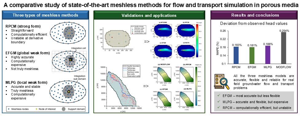
In recent years, meshless methods have been increasingly applied to the simulation of various engineering problems due to their inherent advantages over traditional mesh-based approaches, including greater flexibility, independence from predefined meshing, simpler adaptive analysis, improved automation, and suitability for complex problems. Several meshless methods have been used for porous media simulation, and are broadly categorized into collocation, global weak form and local weak form methods. In this study, a comprehensive comparison of the applicability of these three categories of meshless methods for simulating coupled flow and transport problems in porous media is presented. The Radial Point Collocation Method (RPCM) (strong form), the Element Free Galerkin Method (EFGM) (global weak form) and the Meshless Local Petrov Galerkin (MLPG) method (local weak form) are implemented and systematically compared. These methods are applied to the analysis of flow in a synthetic regular domain aquifer, flow and non-reactive contaminant transport in a synthetic irregular boundary porous media problem and groundwater flow in a field aquifer located in India. The simulated groundwater heads are compared with analytical solution, observed field data and results obtained from widely used MODFLOW-MT3DMS models. The deviation of the solutions from the analytical solution is in the range of 0.67% to 0.16% for the hypothetical case study. For the field-scale case study, mean absolute error of 0.183%, 0.181% and 0.188% are obtained for the RPCM, EFGM and MLPG models, respectively, outperforming MODFLOW, which exhibits a deviation of 0.254% from observed values. Overall, the present study reaffirms the practical applicability of these meshless methods for real-world groundwater problems and provides valuable insights into the utilization of each category of meshless method, with respect to problem type, computational efficiency and accuracy requirements.Graphic Abstract
Keywords
The simulation of groundwater flow and transport is one of the most important porous media problems dealing with large-scale complex aquifer systems. In groundwater problems, the decline in groundwater levels and depletion of groundwater quality are the inevitable consequences of population growth and increasing variability in climatic and precipitation patterns [1,2]. The associated challenges include lowering groundwater table and subsequent drying up of aquifers, reduced discharges to surface water systems, increased salinization, crop deaths and wider spread of pollution [3]. The estimation of spatio-temporal variations of contaminants combined with head changes in the aquifer aids in effective groundwater management plans [4]. Numerical models are extensively used for the assessment and prediction of aquifer behavior [5].
The Finite Difference Method (FDM) and the Finite Element Method (FEM) are among the most widely used numerical techniques in groundwater simulation. Prominent software packages such as MODFLOW [6], MT3DMS [7], SEAWAT [8], MODFLOW-SURFACT [9], and Parameter ESTimation (PEST) [10] are based on the FDM. FEM-based software includes FEFLOW [11] and SUTRA [12]. Despite their broad applicability, these methods have several limitations such as high cost and memory requirements for meshing and remeshing, difficulty in controlling accuracy, misalignment of mesh with problem boundaries, slower simulation speeds, complex preprocessing and reduced accuracy for higher dimensions and advection-dominant problems [13–16].
To overcome the limitations of the mesh-based methods and the development of more powerful tools, meshless methods were first introduced in 1970s [17]. Since 1990s, several meshless methods have been developed and successfully applied for various Partial Differential Equations (PDEs). Based on the formulation of the PDE, the meshless methods can be classified into strong or weak form methods. Collocation or strong form methods employ a collocation technique for the discretization of the governing PDE, and they are simple, truly meshless and computationally efficient [18], though they may suffer from stability issues at Neumann boundaries. On the other hand, weak or integral forms of governing equations are discretized in weak form methods, and these methods have high stability at Neumann boundaries due to the integration process [17]. The weak form methods are further classified as global or local weak form methods according to the utilization of global domain or overlapping local support domains for the integration purpose [13]. Global weak form methods require a background mesh for integration, and hence they are not truly meshless, while local weak form methods, though truly meshless, are typically more computationally intensive [17].
Among the earliest applications of meshless methods in groundwater flow modelling, is the Element Free Galerkin Method (EFGM), a global weak form method [19–21]. Variants of the classical EFG formulation have been developed to enhance the computational efficiency and numerical robustness. For example, complex variable element-free Galerkin method employs complex variable theory to improve the treatment of two-dimensional field problems and reduce the computational complexity [22]. Collocation techniques using Radial Basis Functions (RBF) are applied for transport simulation [23] and unsaturated zone problems [24]. Local Radial Point Interpolation Method (LRPIM) is employed for coastal aquifer flow modelling [25], and Smooth Particle Hydrodynamics (SPH) is applied for modelling contaminant transport in heterogeneous aquifers [26]. In addition, the Generalized Finite Difference Method (GFDM), which constructs local weighted approximations of differential operators over scattered nodes [27–29], has been successfully applied to diffusion and convection–diffusion problems relevant to porous media flow. Meshless formulations based on finite volume concepts, often referred to as extended or meshless finite volume methods (EFVM/MFVM), have also been developed to preserve local mass conservation while retaining geometric flexibility [30,31]. Furthermore, dimension-splitting meshless methods have been introduced to improve computational efficiency by decomposing multidimensional problems into sequential one-dimensional approximations while maintaining solution accuracy [32].
The adoption of meshless methods in groundwater modelling has been increased since 2010. Meenal and Eldho [33] demonstrated the effectiveness of Point Collocation Method (PCM) for the flow simulation in unconfined aquifers, noting excellent similarity of PCM head computations with the solutions of FEM and Boundary Element Method (BEM). However, PCM has a limitation of high sensitivity to the time step and shape function parameters. Kovářík and Mužík [34] utilized the local boundary integral method (LBIEM) for density driven flow estimation and proved that the approximation using RBFs can reduce the computational expense. Li et al. [29] further modelled the density driven flows using generalized finite difference method (GFDM), along with implicit Euler and Newton-Raphson methods to benchmark problems. Swathi and Eldho [35] employed the Meshless Local Petrov Galerkin (MLPG) method, a local weak form method for flow simulation. MLPG was found to be a promising tool, with excellent similarity with PCM and BEM and with better stability. The Radial Point Collocation Method (RPCM) is another widely used meshless method for groundwater flow and transport simulations [36]. Patel and Rastogi [37] validated Kansa’s RBF-based meshless method for field-scale aquifer simulations. Pathania et al. [38] applied EFGM to model spatio-temporal variations of river-aquifer interactions. Anshuman and Eldho [39] extended RPCM for flow and transport of multiple species with linked first-order reactions. Swetha et al. [40] used LRPIM for flow simulations in confined aquifers and verified the model with benchmark problems. The good agreement of LRPIM with FDM and FEM reiterates its use as an alternative modelling tool. Das and Eldho [41] proposed a hybrid meshless weak strong (MWS) form method by integrating MLPG and RPCM, achieving accurate solutions with less computational effort.
This study presents a systematic and formulation-oriented comparison of three representative meshless methods for groundwater flow and contaminant transport simulations. Rather than comparing algorithms arbitrarily, the selected methods are deliberately chosen to represent the three principal theoretical frameworks in meshless discretization: strong form, global weak form, and local weak form. Primary objective of the study is to evaluate and compare the numerical accuracy, stability, and practical applicability of three representative categories of meshless methods for groundwater flow and contaminant transport problems, using both synthetic and field-scale case studies. The strong form RPCM [36,42], global weak form EFGM [43,44] and the local weak form MLPG [35,45] methods have been applied for solving the groundwater flow equation in unconfined aquifers coupled with the transport of dissolved non-reactive contaminants. The weak-form meshless methods, MLPG and EFGM, have enhanced numerical stability through integration of the governing equations, but at the cost of increased computational effort. In contrast, RPCM is simpler and computationally efficient, but it may be unstable for complex problems. The background integration strategies also differ between EFGM and MLPG. EFGM relies on a background mesh for numerical integration, whereas MLPG employs local subdomains for integration, making it truly meshless and more flexible.
Based on the theoretical distinctions of the three proposed methods, the study is guided by three working hypotheses. First, local weak-form MLPG is expected to exhibit improved numerical stability compared to the strong-form RPCM. Second, global weak-form EFGM is anticipated to provide higher accuracy at the expense of increased computational cost relative to collocation-based approaches. Third, all three meshless methods provide an easy option for varying nodal distribution of computational domain and representing complex boundaries, while achieving better performance compared to the standard grid-based MODFLOW-MT3DMS model. In this study, the meshless models are compared with MODFLOW-MT3DMS simulations in cases where real data or analytical solutions are unavailable. As MODFLOW-MT3DMS is widely used in industries, it serves as a reference for demonstrative comparison and consistency verification. Initially, the models are demonstrated using hypothetical case studies with regular and irregular boundaries, and the deviation of heads and concentrations from RPCM, EFGM and MLPG from analytical solution, MODFLOW and MT3DMS solutions are reported. To further test the realistic application, the three meshless models have been applied to the case study of a real aquifer in Telangana, India, and the flow model results are compared with observed groundwater head data and MODFLOW. Thus, this study provides an in-depth evaluation of the strengths and limitations of different meshless methods and establishes their practical utility in the field-scale groundwater modelling.
The governing PDE for a heterogeneous, anisotropic unconfined aquifer is given by [6]:
where, x and y are Cartesian coordinates, h is the unknown groundwater head, Sy is the specific yield, Kx and Ky are hydraulic conductivities, Q represents the point source/sink, δ is Dirac delta function, q is known domain inflow and t is time. The initial condition is given by [6]:
where,
where
The governing advection-dispersion equation in two-dimensions for the non-reactive contaminant transport can be written as [7]:
where, Dxx is the longitudinal dispersion coefficient, Dyy is the transverse dispersion coefficient, vx, and vy are the average linear velocities, and c is the dissolved contaminant concentration. The initial conditions and Dirichlet and Neumann boundary conditions are [7]:
where, c0 is the initial concentration, c1 and f2 are the Dirichlet and Neumann boundary values, respectively. The average linear velocities in two-dimensions
Further, the dispersion coefficient Dxx and Dyy can be computed as [7]:
where,
Here,
The FDM/FEM based models require the discretization of the problem domain into a grid/mesh, with pre-defined connectivity essential for interpolation. Any significant change in external stress conditions or the need for improved accuracy necessitates remeshing, which makes these methods cumbersome. In contrast, the interpolation in meshless methods is performed by the construction of shape function representing heads or concentrations at nodes, inside and on the support domain. In this study, RPCM, EFGM and MLPG models employ Multi-Quadric Radial Basis Function (MQ-RBF), Moving Least Squares (MLS) and Improved Interpolating Moving Least Squares (IIMLS) techniques for the generation of shape functions. The detailed methodology of these approximating techniques is available in [17,46].
RPCM involves collocating the governing equations at nodes and utilizing RBFs for interpolation. It is truly meshless and generates a banded system matrix, making it simple, flexible, and computationally efficient for a wide range of problems. However, RPCM may experience stability issues near Neumann boundaries and require special handling. EFGM, on the other hand, has better stability and a higher convergence rate than RPCM. However, it is not truly meshless and requires a background mesh for the global integration [47]. MLPG is versatile and is truly meshless. The numerical integration in MLPG is performed over small, localized regions, known as integration of sub-domains which are considered as circles centered at nodes [48]. A typical discretization using FDM and three types of meshless methods is illustrated in Fig. 1.

Figure 1: Typical discretization of domain using (a) FDM, (b) RPCM, (c) EFGM and (d) MLPG.
RPCM employs Radial Basis Functions (RBFs) for shape functions (ϕ) construction. Instead of a predefined mesh, the domain is represented by scattered nodes. Each node is associated with a local support domain, within which the shape function is calculated. These local support domains overlap and collectively cover the entire problem domain. Their shape can vary, but in this work, circular support domains are specifically chosen. The size of each support domain is defined relative to the nodal spacing
here
Here, fR is the MQ-RBF, which is given as:
The term
Here,
The term ϕ denotes the shape function, computed for each node within its local support domain. Its directional derivatives are obtained by replacing the MQ-RBF vector (
Similarly, the contaminant transport equation (Eq. (4)) can be discretized as follows:
In this study, the Crank–Nicolson method is applied by setting the parameter θ = 0.5. Eqs. (16) and (17) apply to all the internal nodes. The governing equations, combined with boundary conditions, are assembled into a global matrix–vector system of the form
EFGM uses Galerkin integral approach. In EFGM, the integral form of a governing equation weighted with the MLS shape functions gives a set of linear algebraic equations. This study uses cubic spline weight function and rectangular influence domain to compute the MLS shape functions. Further, dimensionless factor (
On using the trial function
In Eq. (19),
where
On applying EFGM steps to Eq. (21), the following system of equation can be obtained like Eq. (20) for head and solved to get the concentration for the next time step i.e.,
The weak forms of meshless methods usually use a background mesh for integration. The global weak form methods have this issue, which do not make them truly Meshless methods. In MLPG, the integration is done using overlapping of local sub domains. Thus, the MLPG does not need background mesh in any stages of integration and interpolation, which makes it a truly meshless method. In the MLPG method, let the sub-domain be denoted by
where,
Using a penalty factor of α, at the Dirichlet boundary:
The Neumann boundary condition is applied directly as:
here, n represents the normal direction, h1 and
Similarly, the MLPG formulation for contaminant transport can be written as [41]:
where,
The Dirichlet and Neumann boundary conditions are given as:
where, c1 and
The developed RPCM, EFGM and MLPG models for the aquifer flow is integrated with a transport model to form integrated flow and transport model. The flow chart describing the model is given in Fig. 2. The procedure can be described as follows:

Figure 2: Modelling procedure of meshless based coupled flow and transport models.
Step 1: The hydrogeological details, problem domain, meshless parameters, number of nodes and the corresponding arrangement, pumping wells, streams, recharge zones, heterogeneity and anisotropy, initial and boundary conditions are inputted into the meshless models.
Step 2: The size of the support and sub domain are fixed. The sub domain is used for the integration of the MLPG and EFGM models. The support domain is used for the interpolation.
Step 3: The meshless formulations for groundwater flow equation are solved using MATLAB and Python for solving the unknown head values. The RPCM model was developed in Python, while the EFGM and MLPG models were developed in MATLAB. Consistent numerical procedures and solver parameters were maintained across the platforms to ensure comparability of results.
Step 4: The velocity is calculated using the Darcy’s law and the dispersion coefficients are computed using Eqs. (9) and (10).
Step 5: The values computed in step 4 are inputted into the transport model. The meshless transport models are implemented, similar to step 4 and the contamination concentration are computed.
Step 6: The steps 3, 4 and 5 are repeated.
A hypothetical square-shaped confined aquifer with dimensions of 1400 m × 1400 m is considered (Fig. 3a) for validating and comparing the meshless models. Constant boundary conditions of 100 m are imposed along the left and right boundaries, while the top and bottom boundaries are treated as no-flow boundaries. The aquifer transmissivity and storativity are taken as 100 m2/day and 0.001, respectively. A pumping well is located at the center of the domain, with a pumping rate of 10,000 m3/day. The domain is discretized into 225 nodes, and six locations are designated as observation points, as shown in Fig. 3a. The head distribution simulated using the meshless models are compared with the analytical solution proposed by Willis and Yeh [49] at the selected observation wells given in Fig. 3a. The results are presented in Table 1. The head distribution obtained from the MLPG model is illustrated in Fig. 3b, while the other meshless models exhibit identical contour patterns. As evident from the results in Table 1, all meshless models show excellent agreement with the analytical solution. The average errors at the six observation wells are 1.25%, 0.666%, 0.442% and 0.16% for MODFLOW, RPCM, MLPG and EFGM models, respectively. These results establish the reliable performance of all the three meshless models, with the EFGM model showing higher accuracy.

Figure 3: Case study 1 (a) nodal arrangement and (b) head distribution from MLPG model.

In this case study, the three meshless models are applied to a hypothetical unconfined aquifer with an irregular boundary geometry [50]. The aquifer extends 290 m in the x direction and 190 m in the y direction, as shown in Fig. 4a. The aquifer is bounded by Dirichlet boundary on the West and East, with constant head values of 132 and 128 m. The remaining boundaries are considered to be no flow boundaries.

Figure 4: (a) Problem domain, (b) Meshless nodal distribution for the hypothetical case study.
The aquifer is assumed to be homogeneous and isotropic, with a hydraulic conductivity of 5 m/day and an effective porosity of 0.3. Three pumping wells are located at node numbers 76, 294, and 442, each operating at a rate of 200 m3/day. Three recharge wells are located at node numbers 68, 283, and 449, each recharging at a rate of 200 m3/day. A constant Total Dissolved Solids (TDS) concentration of 500 mg/L is introduced at node number 130. The models are simulated over a period of 2 years using a time step of one day to evaluate contaminant concentrations. For meshless simulation, the aquifer domain was discretized using 514 nodes, as shown in Fig. 4b.
Since no analytical solution is available for this case study, a coupled MODFLOW and MT3DMS model is used as a reference rather than for intercomparison. The MODFLOW-MT3DMS model is developed with a uniform grid size of 10 m × 10 m. The performance of the meshless models is evaluated against MODFLOW and MT3DMS using multiple statistical indicators, including average error, Root Mean Square Error (RMSE), Normalized Root Mean Square Error (NRMSE), Nash–Sutcliffe Efficiency (NSE) and L∞ error given by the following equations:
In the Eqs. (32)–(36),
The flow models are first executed, and the steady-state hydraulic head contours obtained from MODFLOW, RPCM, MLPG and EFGM are given in Fig. 5. The local support domain sizes are taken as 3 times the nodal distance for RPCM and MLPG models. The RPCM model parameters which include the MQ-RBF shape parameters i.e., q and α are set as 0.98 and 5, respectively, from the previous literature [39]. The sub-domain size is taken as 0.45 times the nodal spacing in MLPG model [41]. The dimensionless size of the influence domain αi of EFGM is taken as 1. The groundwater head values comparison at twelve points are provided in Tables 2 and 3. The results reveal close agreement between the meshless models and the MODFLOW solutions. Further, heads from the flow model are used to compute nodal velocities and dispersion coefficients, which are then used as inputs to the transport model.

Figure 5: Distribution of the groundwater head from the four models for hypothetical aquifer.


The concentration contours after 2 years are estimated and plotted as shown in Fig. 6. The breakthrough curves, representing the variation of concentration over the simulation time, at nodes 170, 190, 210 and 230 are shown in Fig. 7. As observed from these plots, there is close agreement among the RPCM, EFGM, MLPG and MT3DMS models. Thus, the proposed meshless models are demonstrated to be reliable for simulating the flow and transport in the porous media.

Figure 6: Concentration distribution after 2 years from the four models for the hypothetical aquifer.

Figure 7: Breakthrough curves at four nodes (a) Node 170 (b) Node 190 (c) Node 210 and (d) Node 230 from the four models for case study 2.
As meshless parameters strongly influence the model performance, a sensitivity analysis is conducted. The RBF shape parameters q and α of the RPCM model are varied around the base case (q = 0.98, α = 5) with q = 0.5 and α = 1, 2, 3, and 7. Similarly, support domain size of EFGM, support and sub domain radii of MLPG are varied as 0.3 and 0.45 to demonstrate the model performance under varying meshless parameters. The results as shown in Fig. 8a show that the transport solution is more sensitive to reduction in q, which increases numerical diffusion and alter breakthrough behavior, whereas moderate variations in α produce comparatively smaller deviations. From Fig. 8b,c, it can be observed that solutions are stable within a recommended parameter range [38,51]. In addition, the three meshless models are tested under varying time steps of 0.5 day, 1 day and 2 days, as shown in Fig. 8d–f. The solutions remain stable for time steps up to Δt = 2 days, as shown in the breakthrough curves at four observation nodes. Thus, this analysis aids in parameter selection and demonstrates the robustness of the models within the recommended ranges [38,39,51]. However, model sensitivity outside these ranges can significantly impact the performance, often necessitating a trial-and-error approach for optimal parameter calibrations.

Figure 8: Performance of the meshless models under varying parameters. (a) RPCM model response to variations in RBF shape parameters, (b) MLPG model response to changes in the ratios of support domain radius (R) and sub-domain radius (r) relative to nodal spacing (L), (c) EFGM model response to variations in size of the influence domain (αi), (d) RPCM model performance under varying time steps, (e) MLPG model performance under varying time steps, (f) EFGM model performance under varying time steps.
To evaluate the applicability of meshless methods for large-scale field problems, the RPCM, EGFM and MLPG models are applied to a large, field unconfined aquifer located in the Patancheru industrial development area of Telangana, India for groundwater flow simulation (Fig. 9). The site information details are available in [52,53].

Figure 9: Problem domain of the field-scale study.
The study area contains two streams, Nakkavagu and Pedhavagu, and a comprehensive groundwater level monitoring was conducted in this area during 1997 [52]. The area of the aquifer is approximately 93 km2 and its thickness is 15 m. All the boundaries of domain are Neumann boundaries with zero flux. There are 15 observation wells in the aquifer. The aquifer domain is illustrated in Fig. 9. The groundwater recharge is taken from precipitation of 110 mm/year, and the seepage from the stream is considered to be 130 mm/year. The initial value of hydraulic conductivity of 62.5 m/day is modified to 60 m/day during the calibration for improved model accuracy. There are 189 bore wells in the study area, each extracting groundwater at a rate of 95 m3/d and operating for 60% of the day [53].
A uniformly distributed arrangement of 1597 nodes with 250 m nodal spacing are considered for the meshless simulation. The meshless model parameters are kept similar to the case study 2. The spatial distribution of meshless nodes and the locations of the bore wells are shown in Fig. 10.

Figure 10: Meshless nodal arrangement for the field-scale case study using MODFLOW, RPCM, EFGM and MLPG models.
The meshless flow models for unconfined aquifer are first executed to obtain a steady state head distribution for the year 1997. The velocities over the aquifer domain are computed using Darcy’s law given in Eq. (9). The simulated head values obtained from the meshless model are compared with observed head values [52]. Additionally, widely used MODFLOW is applied to establish a reference model for transient state simulation, rather than for direct comparison of meshless solutions. The solutions are assessed using average error, RMSE, NRMSE, NSE and L∞ error.
The contour plots of the head distribution are shown in Fig. 11 using the MODFLOW, RPCM, EFGM and MLPG models. The flow direction is observed to be from the southeast to the northwest, following the gradient from higher to lower hydraulic heads. The comparison of head at observation wells from MODFLOW and meshless models with the actual head values are given in Tables 4 and 5. It can be observed that meshless solutions are in excellent agreement with the observed head values and are slightly more accurate than the MODFLOW model. The low average error, RMSE, NRMSE, L∞ error and NSE values are closer to 1 indicating the effectiveness of the MLPG flow simulation model. Additionally, the meshless model has better reusability due to easier adaptive analysis.

Figure 11: Groundwater head distribution in 1997 using MODFLOW, RPCM, EFGM and MLPG models.


Subsequently, RPCM, EFGM and MLPG flow models are executed in transient state conditions, and head distribution in 2025 is generated. Thus, the transient state models are executed for 28 years, with a time step of 14 days, with an assumption that the stress remains constant. The MODFLOW simulation is implemented with the same parameters. The head distributions in 2025 obtained from the MODFLOW, RPCM, EFGM and MLPG models are shown in Fig. 12. The meshless solutions indicate a closer similarity among the meshless models and MODFLOW. Also, head distribution in 2025 is close to that in 1997, due to the constant minimal stresses and attainment of steady state under the assumed conditions.

Figure 12: Groundwater head distribution in 2025 using four models.
Further, high pumping rate of 3000 m3/day is considered at each of the pumping wells to evaluate the model response under hypothetical transient stressed conditions. Using the 2025 head distribution as the initial condition, transient simulations are run for one-year period. The value of αi is taken as 2. As shown in Fig. 13, meshless model results are in close agreement with the standard MODFLOW model simulations.

Figure 13: Groundwater head distribution under hypothetical stressed conditions using four models.
In this study, the performance and efficiency of three categories of meshless methods are evaluated for the simulation of groundwater flow and transport processes. The RPCM, EFGM and MLPG based flow and transport models, previously developed by the authors [39,41,44], are applied to three representative case studies and their results are systematically intercompared. The widely used grid-based MODFLOW-MT3DMS model is adopted as a reference model and implemented using similar spatial and temporal discretization to ensure consistency in comparison.
In the first case study, model results are compared with an analytical solution, and all three meshless models show excellent agreement with the EFGM model providing the highest accuracy. In the second case study, involving a hypothetical unconfined aquifer with an irregular boundary, the MODFLOW-MT3DMS, RPCM, EFGM, and MLPG models are successfully applied for the simulation of head and TDS concentration over a two year period. Among the meshless models, EFGM and MLPG exhibit the closest agreement with MODFLOW results, with average head deviations of 0.062% and 0.066%, respectively. The best overall performance across all statistical evaluation measures is demonstrated by the EFGM model, followed by MLPG model. RPCM model also perform reliably, with an average deviation of 0.179%. The simulated concentration contours after two years indicated good agreement among the four models. However, from the breakthrough curve analysis, an overestimation of concentration values is observed for the EFGM and RPCM models, whereas a slight deviation in the contaminant trend is observed for MLPG model at certain observation points. With respect to computational efficiency, simulations conducted on a Windows 10 platform with an Intel i7 processor and 16 GB RAM require approximately 7, 10.44, and 9.21 s for RPCM, EFGM, and MLPG models, respectively. The lower computational cost of RPCM model is associated with its strong-form formulation, whereas the increased simulation time for EFGM and MLPG models arises from numerical integration procedures involved in the simulation. These observations support the first and second hypotheses, as the weak-form EFGM and MLPG models demonstrated improved numerical agreement relative to the strong-form RPCM under irregular boundary conditions and EFGM achieved higher accuracy at the expense of greater computational effort.
In the third case study, the applicability of meshless models is demonstrated using a field-scale aquifer system located in Telangana, India. To facilitate comparison, observed groundwater level data has been used and MODFLOW is used as a reference model for transient state simulation. The aquifer system, covering approximately 93 km2 and including 189 borewells and two streams, is used to assess the applicability of the meshless approaches under realistic hydrogeological conditions. The analysis is limited to flow simulation, with the objective of demonstrating large-domain applicability and direct comparison with available observations. For steady-state conditions corresponding to the year 1997, EFGM model demonstrated the best performance, with an average deviation of 0.101%, followed by the RPCM and MLPG models with average deviations of 0.183% and 0.188%, respectively. The MLPG model exhibits lowest L∞ error, indicating that maximum pointwise deviation between simulated and observed heads is minimal. The field-scale results provide evidence in support of the third hypothesis, as all three meshless methods are in close agreement with the observed groundwater heads and MODFLOW model under realistic hydrogeological conditions. A steady-state condition is attained under the considered assumptions, with no significant deviation in head values. Further, a hypothetical stressed scenario with high pumping rates is implemented to assess the transient condition. The meshless models’ simulations demonstrate close agreement with the MODFLOW results. However, the time-varying pumping and recharge play a critical role in governing real-world groundwater dynamics. While the primary focus of the present work is methodological development and comparative evaluation of meshless modelling approaches under controlled conditions, incorporation of temporally variable stresses is essential for realistic system representation. Coupling the proposed framework with time-dependent recharge and pumping data would therefore constitute further extension of this research towards practical, real-world applications.
In this study, the characteristics of three meshless methods are demonstrated. RPCM, as a strong form approach, is characterized by low computational cost and reliable performance. However, as previously reported [41] unstable solutions may be encountered in the presence of Neumann boundary conditions for certain nodal arrangements. The weak form methods such as EFGM and MLPG were found to be very effective in dealing with Neumann boundary conditions, supporting the first hypothesis. In the present study, the most accurate results are consistently obtained using EFGM, but it is not truly meshless, and requires a background mesh for numerical integration. MLPG model is found to provide accurate and stable solutions, but increased computational effort is required due to the local integration process. Thus, the findings indicate that formulation significantly influences numerical stability and efficiency, thereby validating the hypothesis-driven framework adopted in this study. For the solution of a particular problem, based on accuracy requirements, and computational efforts, a particular model may be chosen, depending on the familiarity and requirements of the user.
In this study, a comprehensive evaluation of three meshless methods of different formulation categories is demonstrated for the simulation of groundwater flow and solute transport processes. The primary focus is to compare the applicability, advantages, and limitations of the meshless approaches. The strong-form RPCM, global weak-form EFGM, and local weak-form MLPG methods are employed for this purpose. The governing equations are formulated directly in RPCM, whereas numerical integration is required for EFGM and MLPG approaches. In EFGM, integration is performed using a background mesh, while local circular subdomains are used for the integration in MLPG.
The proposed models are evaluated using a simple square domain aquifer, a hypothetical aquifer with an irregular boundary and a field-scale aquifer system. In all cases, excellent agreement is observed with the analytical solution and observed groundwater level data. The purpose of the MODFLOW-MT3DMS model in this study is to serve as a reference framework where analytical solutions or observed data are unavailable, rather than to establish superiority or inferiority relative to meshless approaches. Among the three models, EFGM provides higher accuracy but with maximum computational cost. RPCM and MLPG models also provide reliable solutions. For flow simulations, deviations of less than 0.6% are observed for all three meshless models when compared with the analytical solution, observed data and MODFLOW results. EFGM and MLPG are more effective in handling Neumann boundary conditions than RPCM. RPCM is computationally efficient and well suited for the Dirichlet boundary problems. With the requirement of background mesh and numerical integration, EFGM exhibits reduced flexibility compared to RPCM and MLPG. Overall, the results confirm the effectiveness and applicability of the three meshless methods for groundwater flow and transport modelling across both small-scale and large-scale porous media problems.
The following are some of the limitations of the study. The comparative performance of the meshless methods is assessed only for the case studies considered, and variations in the relative performance, particularly between EFGM and MLPG, may arise under different hydrogeological conditions. The meshless models are found to be sensitive to the sizes of the support and subdomains and require tuning to achieve optimal results. In the field-scale case study, some of the adopted assumptions cause simplifying representation of climate variability and anthropogenic influences on the groundwater system. Incorporating time-varying field stresses, ideally through coupling with a hydrological model, represents an important extension of the present work and enables more realistic simulation of transient, real-world groundwater systems. Nevertheless, the results demonstrate the potential of meshless methods to evolve into reliable groundwater modelling tools, either as standalone approaches or in combination with grid-based models.
Acknowledgement: Not applicable.
Funding Statement: The authors received no specific funding for this study.
Author Contributions: The authors confirm contribution to the paper as follows: Conceptualization: T. I. Eldho; methodology: T. I. Eldho; software: Sanjukta Das, Aatish Anshuman and Tinesh Pathania; validation: Sanjukta Das, Aatish Anshuman and Tinesh Pathania; formal analysis: Sanjukta Das, Aatish Anshuman and Tinesh Pathania; investigation: Sanjukta Das, Aatish Anshuman and Tinesh Pathania; resources: T. I. Eldho, Sanjukta Das, Aatish Anshuman and Tinesh Pathania; data curation: Sanjukta Das, Aatish Anshuman and Tinesh Pathania; writing—original draft preparation: Sanjukta Das; writing—review and editing: T. I. Eldho; visualization: Sanjukta Das; supervision: T. I. Eldho. All authors reviewed and approved the final version of the manuscript.
Availability of Data and Materials: The data that support the findings of this study are available from the corresponding author, T. I. Eldho, upon reasonable request.
Ethics Approval: Not applicable.
Conflicts of Interest: The authors declare no conflicts of interest.
References
1. van Rooyen J, Watson AP, Miller JA. Combining quantity and quality controls to determine groundwater vulnerability to depletion and deterioration throughout South Africa. Environ Earth Sci. 2020;79(11):255. doi:10.1007/s12665-020-08998-1. [Google Scholar] [CrossRef]
2. Dangar S, Asoka A, Mishra V. Causes and implications of groundwater depletion in India: a review. J Hydrol. 2021;596:126103. doi:10.1016/j.jhydrol.2021.126103. [Google Scholar] [CrossRef]
3. Jomaa I. The role of groundwater depletion in local and global climate change. Zenodo. 2025. doi:10.5281/zenodo.15192267. [Google Scholar] [CrossRef]
4. Palma M, Maggio S, Cappello C, Congedi A, De Iaco S. Spatio-temporal modeling of groundwater quality deterioration and resource depletion. Hydrogeol J. 2023;31(6):1443–61. doi:10.1007/s10040-023-02692-9. [Google Scholar] [CrossRef]
5. Shakeri R, Nassery HR, Ebadi T. Numerical modeling of groundwater flow and nitrate transport using MODFLOW and MT3DMS in the Karaj alluvial aquifer. Iran Environ Monit Assess. 2022;195(1):242. doi:10.1007/s10661-022-10881-4. [Google Scholar] [PubMed] [CrossRef]
6. Langevin CD, Hughes JD, Banta ER, Niswonger RG, Panday S, Provost AM. Documentation for the MODFLOW 6 groundwater flow model (No. 6-A55). Reston, VA, USA: US Geological Survey; 2017. doi:10.3133/tm6A55. [Google Scholar] [CrossRef]
7. Zheng C, Hill MC, Cao G, Ma R. MT3DMS: model use, calibration, and validation. Trans ASABE. 2012;55(41549–59. doi:10.13031/2013.42263. [Google Scholar] [CrossRef]
8. Guo W, Langevin CD. User’s guide to SEAWAT: a computer program for simulation of three-dimensional variable-density ground-water flow. Vol. 1. Reston, VA, USA: US Geological Survey; 2002. doi:10.3133/twri06A7. [Google Scholar] [CrossRef]
9. Panday S, Huyakorn PS. MODFLOW SURFACT: a state-of-the-art use of vadose zone flow and transport equations and numerical techniques for environmental evaluations. Vadose Zone J. 2008;7(2):610–31. doi:10.2136/vzj2007.0052. [Google Scholar] [CrossRef]
10. Doherty J. PEST: a unique computer program for model-independent parameter optimisation. In: Water down under 94: groundwater/surface hydrology common interest papers; preprints of papers. Barton, Australia: Institution of Engineers, Australia; 1994. p. 551–4. [Google Scholar]
11. Diersch HJG. FEFLOW: finite element modeling of flow, mass and heat transport in porous and fractured media. New York, NY, USA: Springer Science & Business Media; 2013. [Google Scholar]
12. Voss CI, Provost AM. SUTRA: a model for 2D or 3D saturated-unsaturated, variable-density ground-water flow with solute or energy transport. Reston, VA, USA: US Geological Survey; 2002. Report No.: 2002-4231. doi:10.3133/wri024231. [Google Scholar] [CrossRef]
13. Nguyen VP, Rabczuk T, Bordas S, Duflot M. Meshless methods: a review and computer implementation aspects. Math Comput Simul. 2008;79(3):763–813. doi:10.1016/j.matcom.2008.01.003. [Google Scholar] [CrossRef]
14. Niraula P, Han Y, Wang J. Comparison of meshfree and mesh-based methods for boundary value problems in physics. J Phys Conf Ser. 2015;640(1):012067. doi:10.1088/1742-6596/640/1/012067. [Google Scholar] [CrossRef]
15. Mazhar F, Javed A, Xing JT, Shahzad A, Mansoor M, Maqsood A, et al. On the meshfree particle methods for fluid-structure interaction problems. Eng Anal Bound Elem. 2021;124:14–40. doi:10.1016/j.enganabound.2020.11.005. [Google Scholar] [CrossRef]
16. Suchde P, Jacquemin T, Davydov O. Point cloud generation for meshfree methods: an overview. Arch Comput Meth Eng. 2023;30(2):889–915. doi:10.1007/s11831-022-09820-w. [Google Scholar] [CrossRef]
17. Liu GR, Gu YT. An introduction to meshfree methods and their programming. New York, NY, USA: Springer Science & Business Media; 2005. doi:10.1007/1-4020-3468-7. [Google Scholar] [CrossRef]
18. Jiang W, Gao X. Review of collocation methods and applications in solving science and engineering problems. Comput Model Eng Sci. 2024;140(1):41–76. doi:10.32604/cmes.2024.048313. [Google Scholar] [CrossRef]
19. Park YC, Leap DI. Modeling groundwater flow with a free and moving boundary using the element-free Galerkin (EFG) method. Geosci J. 2000;4(3):243–9. doi:10.1007/BF02910142. [Google Scholar] [CrossRef]
20. Sakurai H, Kawahara M. Three-dimensional groundwater flow analysis system using the element-free Galerkin method. Int J Comput Fluid Dyn. 2004;18(4):309–15. doi:10.1080/1061856031000152326. [Google Scholar] [CrossRef]
21. Kumar RP, Dodagoudar GR, Rao BN. Meshfree modelling of one-dimensional contaminant transport in unsaturated porous media. Geomech Geoengin. 2007;2(2):129–36. doi:10.1080/17486020701379302. [Google Scholar] [CrossRef]
22. Cheng YM, Li RX, Peng MJ. Complex variable element-free Galerkin method for viscoelasticity problems. Chin Phys B. 2012;21(9):090205. doi:10.1088/1674-1056/21/9/090205. [Google Scholar] [CrossRef]
23. Leopold V, Goran T, Franc R. A comparison of the effectiveness of using the meshless method and the finite difference method in geostatistical analysis of transport modeling. Int J Comput Methods. 2005;2(2):149–66. doi:10.1142/s0219876205000405. [Google Scholar] [CrossRef]
24. Ku CY, Hong LD, Liu CY, Xiao JE. Space–time polyharmonic radial polynomial basis functions for modeling saturated and unsaturated flows. Eng Comput. 2022;38(6):4947–60. doi:10.1007/s00366-021-01519-z. [Google Scholar] [CrossRef]
25. Oruç Ö. An extrapolated second-order BDF combined with local meshfree radial point interpolation method for numerical simulation of multi-dimensional regularized long wave equation emerging in fluids. J Sci Comput. 2025;104(2):44. doi:10.1007/s10915-025-02948-4. [Google Scholar] [CrossRef]
26. Jiao T, Ye M, Song J, Yang J, Yin M. An adaptive SPH method (ADP-SPH) for simulating solute transport in heterogeneous aquifers. Water Resour Res. 2025;61(12):e2025WR040299. doi:10.1029/2025wr040299. [Google Scholar] [CrossRef]
27. Benito JJ, Ureña F, Gavete L. Influence of several factors in the generalized finite difference method. Appl Math Model. 2001;25(12):1039–53. doi:10.1016/s0307-904x(01)00029-4. [Google Scholar] [CrossRef]
28. Chávez-Negrete C, Domínguez-Mota FJ, Román-Gutiérrez R. Interface formulation for generalized finite difference method for solving groundwater flow. Comput Geotech. 2024;166(12):105990. doi:10.1016/j.compgeo.2023.105990. [Google Scholar] [CrossRef]
29. Li PW, Fan CM, Chen CY, Ku CY. Generalized finite difference method for numerical solutions of density-driven groundwater flows. Comput Model Eng Sci. 2014;101:319–50. doi:10.3970/cmes.2014.101.319. [Google Scholar] [CrossRef]
30. McLoone M, Quinlan NJ. Coupling of the meshless finite volume particle method and the finite element method for fluid–structure interaction with thin elastic structures. Eur J Mech B. 2022;92(1):117–31. doi:10.1016/j.euromechflu.2021.12.001. [Google Scholar] [CrossRef]
31. Rao X, Zhao H, Liu Y. A novel meshless method based on the virtual construction of node control domains for porous flow problems. Eng Comput. 2024;40(1):171–211. doi:10.1007/s00366-022-01776-6. [Google Scholar] [CrossRef]
32. Sun F, Wang J, Wei Q, Wu Y. An improved meshless method based on the dimension splitting moving least-squares method for elasticity problems. Eng Anal Bound Elem. 2023;150:374–84. doi:10.1016/j.enganabound.2023.02.025. [Google Scholar] [CrossRef]
33. Meenal M, Eldho TI. Simulation of groundwater flow in unconfined aquifer using meshfree point collocation method. Eng Anal Bound Elem. 2011;35(4):700–7. doi:10.1016/j.enganabound.2010.12.003. [Google Scholar] [CrossRef]
34. Kovářík K, Mužík J. A meshless solution for two dimensional density-driven groundwater flow. Eng Anal Bound Elem. 2013;37(2):187–96. doi:10.1016/j.enganabound.2012.10.005. [Google Scholar] [CrossRef]
35. Swathi B, Eldho TI. Groundwater flow simulation in unconfined aquifers using meshless local Petrov–Galerkin method. Eng Anal Bound Elem. 2014;48(1):43–52. doi:10.1016/j.enganabound.2014.06.011. [Google Scholar] [CrossRef]
36. Singh LG, Eldho TI, Kumar AV. Coupled groundwater flow and contaminant transport simulation in a confined aquifer using meshfree radial point collocation method (RPCM). Eng Anal Bound Elem. 2016;66(1):20–33. doi:10.1016/j.enganabound.2016.02.001. [Google Scholar] [CrossRef]
37. Patel S, Rastogi AK. Meshfree multiquadric solution for real field large heterogeneous aquifer system. Water Resour Manag. 2017;31(9):2869–84. doi:10.1007/s11269-017-1668-8. [Google Scholar] [CrossRef]
38. Pathania T, Bottacin-Busolin A, Rastogi AK, Eldho TI. Simulation of groundwater flow in an unconfined sloping aquifer using the element-free Galerkin method. Water Resour Manag. 2019;33(8):2827–45. doi:10.1007/s11269-019-02261-4. [Google Scholar] [CrossRef]
39. Anshuman A, Eldho TI. Meshfree radial point collocation-based coupled flow and transport model for simulation of multispecies linked first order reactions. J Contam Hydrol. 2020;229:103582. doi:10.1016/j.jconhyd.2019.103582. [Google Scholar] [PubMed] [CrossRef]
40. Swetha K, Eldho TI, Singh LG, Kumar AV. Groundwater flow simulation in a confined aquifer using Local Radial Point Interpolation Meshless method (LRPIM). Eng Anal Bound Elem. 2022;134:637–49. doi:10.1016/j.enganabound.2021.11.004. [Google Scholar] [CrossRef]
41. Das S, Eldho TI. A meshless weak–strong form method for the simulation of coupled flow and contaminant transport in an unconfined aquifer. Transp Porous Medium. 2022;143(3):703–37. doi:10.1007/s11242-022-01805-4. [Google Scholar] [CrossRef]
42. Liu X, Liu GR, Tai K, Lam KY. Radial point interpolation collocation method (RPICM) for partial differential equations. Comput Math Appl. 2005;50(8–9):1425–42. doi:10.1016/j.camwa.2005.02.019. [Google Scholar] [CrossRef]
43. Belytschko T, Lu YY, Gu L. Element-free Galerkin methods. Numer Meth Eng. 1994;37(2):229–56. doi:10.1002/nme.1620370205. [Google Scholar] [CrossRef]
44. Pathania T, Eldho TI. A moving least squares based meshless element-free Galerkin method for the coupled simulation of groundwater flow and contaminant transport in an aquifer. Water Resour Manag. 2020;34(15):4773–94. doi:10.1007/s11269-020-02689-z. [Google Scholar] [CrossRef]
45. Atluri SN, Zhu T. A new Meshless Local Petrov-Galerkin (MLPG) approach in computational mechanics. Comput Mech. 1998;22(2):117–27. doi:10.1007/s004660050346. [Google Scholar] [CrossRef]
46. Wang JF, Sun FX, Cheng YM. An improved interpolating element-free Galerkin method with a nonsingular weight function for two-dimensional potential problems. Chin Phys B. 2012;21(9):090204. doi:10.1088/1674-1056/21/9/090204. [Google Scholar] [CrossRef]
47. Hajiazizi M, Bastan P. The elastoplastic analysis of a tunnel using the EFG method: a comparison of the EFGM with FEM and FDM. Appl Math Comput. 2014;234:82–113. doi:10.1016/j.amc.2014.02.024. [Google Scholar] [CrossRef]
48. Atluri SN. The Meshless method (MLPG) for domain and BIE discretizations. Forsyth, GA, USA: Tech Science Press; 2004. [Google Scholar]
49. Willis R, Yeh WG. Groundwater systems planning and management. Englewood Cliffs, NJ, USA: Prentice Hall; 1987. [Google Scholar]
50. Cyriac R, Rastogi AK. Optimization of pumping policy using coupled finite element-particle swarm optimization modelling. ISH J Hydraul Eng. 2016;22(1):88–99. doi:10.1080/09715010.2015.1080126. [Google Scholar] [CrossRef]
51. Das S, Eldho TI. Simulation of reactive transport in porous media using Meshless Local Petrov Galerkin (MLPG) and combination of Meshless Weak and Strong (MWS) form methods. J Contam Hydrol. 2022;251(4):104104. doi:10.1016/j.jconhyd.2022.104104. [Google Scholar] [PubMed] [CrossRef]
52. Gurunadha Rao VVS, Dhar RL, Subrahmanyam K. Assessment of contaminant migration in groundwater from an industrial development area, Medak district, Andhra Pradesh, India. Water Air Soil Pollut. 2001;128(3):369–89. doi:10.1023/A:1010307026457. [Google Scholar] [CrossRef]
53. Swathi B. Simulation-optimization models based on meshless and swarm intelligence techniques for groundwater management and remediation [dissertation]. Mumbai, India: IIT Bombay; 2017. [Google Scholar]
Cite This Article
 Copyright © 2026 The Author(s). Published by Tech Science Press.
This work is licensed under a Creative Commons Attribution 4.0 International License , which permits unrestricted use, distribution, and reproduction in any medium, provided the original work is properly cited.
 Downloads
 Citation Tools
