
 Login
Login Register
 Submit a Paper
 Propose a Special lssue
 Open Access
ARTICLE

Computer Modelling of Thin, Soft Biological Tissues: A Decoupled Strategy for Standardizing Isotropic and Anisotropic Corneal Biomechanics
1 Departamento de Estructuras, Construcción y Expresión Gráfica, Universidad Politécnica de Cartagena member of European University of Technology EUT+, Campus Muralla del Mar, C/Doctor Fleming, s/n, Cartagena, España
2 Grupo de Bioingenieria y Simulación Computacional Aplicada, Universidad Politécnica de Cartagena member of European University of Technology EUT+, Campus Muralla del Mar, C/Doctor Fleming, s/n, Cartagena, España
3 ICA, Université de Toulouse, UPS, INSA, ISAE-SUPAERO, MINES-ALBI, CNRS, 3 rue Caroline Aigle, Toulouse, France
* Corresponding Author: Francisco Cavas. Email:
(This article belongs to the Special Issue: Advances in Modeling and Optimization of Biological and Bio-Inspired Systems)
Computer Modeling in Engineering & Sciences 2026, 148(1), 13 https://doi.org/10.32604/cmes.2026.082643
Received 19 March 2026; Accepted 30 June 2026; Issue published 27 July 2026
 View Full Text
 Download PDF
Abstract
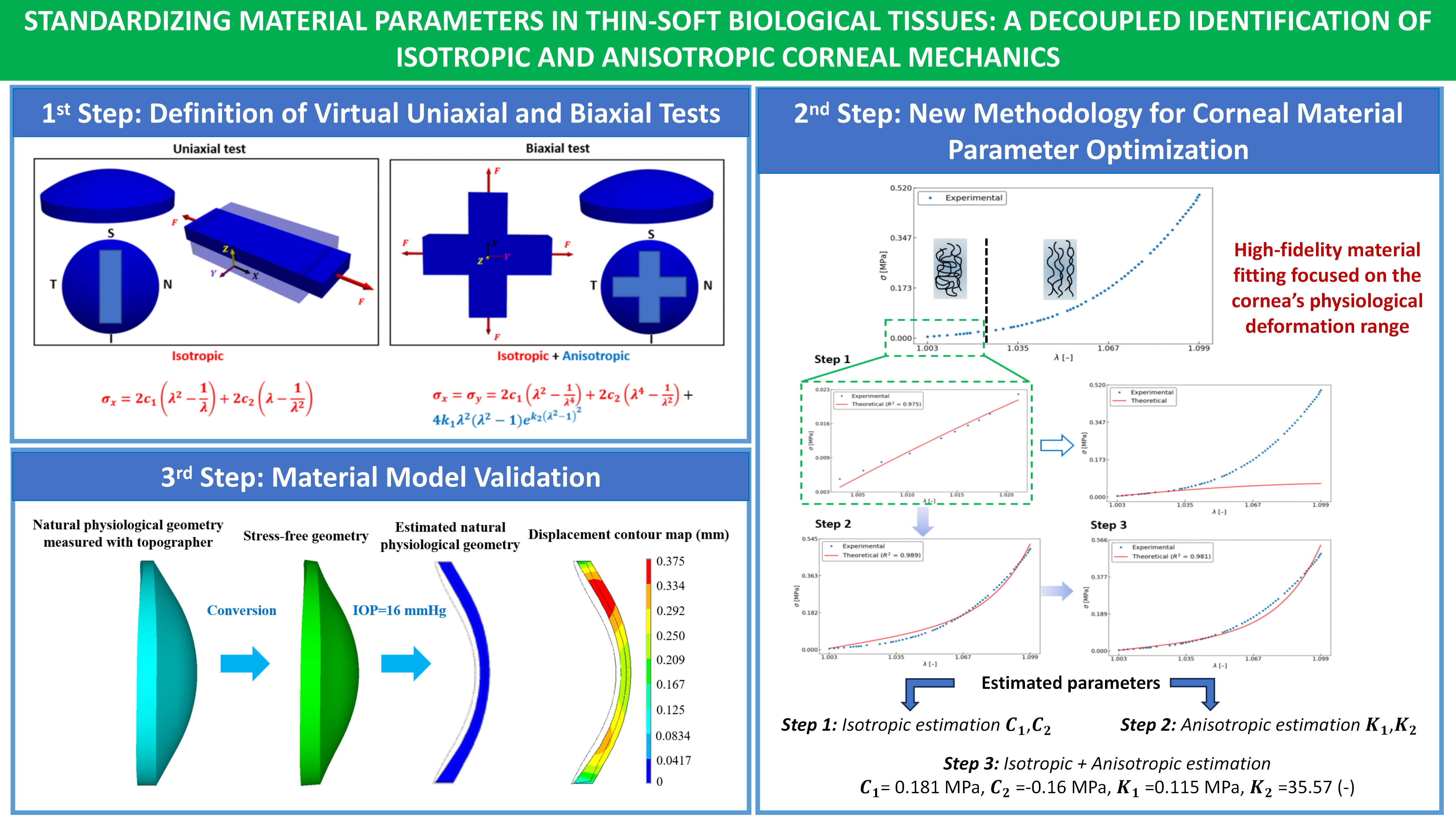
The development of accurate digital twin models of the human cornea is a key factor for planning and monitoring eye treatments and clinical supervision. Corneal tissue can be simulated with the implementation of hyperelastic models based on strain energy density functions. However, the number of hyperelastic models and the parameters’ variation that define these models hinder comparison across different studies. Furthermore, parameter calculations based on a single test are an ill-posed problem. In this research, a novel sequential methodology based on collagen fibril crimping strain threshold has been implemented to calculate the corneal material’s parameters. As an application case, this method has been applied to a hyperelastic Holzapfel–Gasser–Ogden (HGO) model to calculate the isotropic parameters associated with low stretch levels and the anisotropic parameters that consider the collagen fibres’ contribution at higher deformations. The sequential test combination applied to a standardized hyperelastic material model could contribute to ensuring physically meaningful and consistent material parameters, the comparison of different investigations, and the development of an accurate in silico patient-specific cornea model for clinical applications.Graphic Abstract
Keywords
The human cornea is a thin tissue that adopts an aspherical shape as a result of a delicate balance among geometry, intraocular pressure, external loads, boundary conditions, and material mechanical properties, whose characterization is a key factor for the development of accurate patient-specific computational analysis [1] with the integration of material models.
Among available material models, the use of anisotropic hyperelastic models based on the integration of fiber is widely accepted. This assumption is supported by evidence from several studies [2] demonstrating that the collagen fibers contained in the lamellae of the corneal stroma are parallel within each lamella and vary across lamellae. These fibers show preferential nasal–temporal and superior–inferior orientations in the central cornea, which are maintained toward the limbal region, where collagen fibers adopt a preferential circumferential arrangement [3]. Loss of such preferential organization is associated with diseases such as keratoconus [4,5] in which the degradation of mechanical properties leads to corneal bulging and results in severe visual impairment [6].
The first anisotropic hyperelastic models for soft tissues evolved from the exponential formulation proposed by Fung [7], in which the strain-energy density function is expressed in terms of the components of the Green–Lagrange strain tensor without explicitly introducing fiber orientation. This approach captures the global nonlinear response of the tissue from a purely phenomenological perspective, but the parameters lack physical meaning [8]. Additionally, the large number of parameters hinders their identification and may lead to non-polyconvex solutions that compromise model stability [9,10].
The development of invariant-based models represented a significant advancement in incorporating the contribution of fibrillar tissue components and remains the most widely used approach [9,10]. In such models, the free energy is decomposed into an isotropic part, corresponding to the extracellular matrix, and an anisotropic part, dependent on invariants associated with fiber directions. The inclusion of invariants in corneal analysis
Formulations inspired by the Holzapfel–Gasser–Ogden (HGO) model [10] have been successfully adapted to corneal biomechanics, where two principal orthogonally oriented fiber families define stromal anisotropy [11]. These models offer an optimal balance between mathematical simplicity, numerical stability, and predictive capability, and they have therefore become the methodological standard for comparing experimental data and computational simulations in corneal biomechanics [1]. Their main limitations stem from the assumption of perfectly aligned fibers, which may overestimate stiffness in regions where angular dispersion is significant [10], the need to work in a limited range of deformation [12], and the need to be adapted in case of compression analysis [13]; however, their modular structure allows extensions to incorporate dispersion when structural data are available.
More recent models incorporate fiber dispersion through statistical distributions of collagen orientations [14], providing the most faithful representation of corneal microarchitecture. This approach can be formulated using angular integration (AI), where macroscopic response is obtained from an angular distribution function (e.g., von Mises, beta, or Gaussian), or through the generalized structure tensor (GST), which summarizes dispersion into an effective tensor [15,16]. In the cornea, these models allow reproducing regional variations in mechanical behavior and the influence of fibrillar architecture in conditions such as keratoconus [6]. Nevertheless, they require histological or small-angle X-ray scattering (SAXS) data to parameterize dispersion [17] and entail the development of new methodologies for assessing collagen fiber organization [18]. Furthermore, their numerical resolution can be computationally demanding when angular integration is explicitly implemented.
In our previous study [19] a stepwise identification process was proposed to reduce coupling between isotropic and anisotropic components showing that multiple parameter combinations can reproduce the same experimental tests, leading to non-unique but physically plausible solutions showing that direct material’s parameter sets calculation based on single tests is an ill-posed problem [20] and isotropic and anisotropic effects may compensate each other during optimization due to the nonlinear material behavior [21] being necessary the implementation of parametric analysis [22]. Furthermore, the combination of different IOP with parameter sets can reproduce similar results [23].
This lack of uniqueness hinders comparison between studies and limits the comparison between biomechanical models, necessitating the establishment of a standardized protocol to compare the results from different investigations adapted to the physiological stress state of the cornea that works as membranes submitted to a biaxial state due to the intraocular pressure effect.
This study proposes a unified comparative framework for the calculation of material parameters by employing the Holzapfel–Gasser–Ogden (HGO) model due to mathematical simplicity and predictive capacity, and a novel protocol based on a strain threshold for sequential parameter identification. The establishment of a strain threshold can be useful to consider the influence of matrix and fibers contribution allowing at low strain level, where fibers contribution is negligible, the use of uniaxial and equi-biaxial tests results for isotropic parameters calculation considering test coupons cut in any direction whereas uniaxial and equi-biaxial tests results considering superior-inferior and nasal-temporal directions can be used to calculate the anisotropic parameter with strain values exceeding the threshold. The calculation is improved with the implementation of an optimization process based on weighted functions to increase the accuracy in the physiological intraocular pressure range [21], considering data tests based on strain rates close to physiological states [24].
The development of this novel methodology may contribute to the establishment of a robust and efficient common framework for the comparison and validation of experimental data that can be adapted to incorporate dispersion when structural data are available and the definition of different material types for in silico, patient-specific biomechanical cornea models.
In this research, a structural methodology is proposed to optimise the material parameters of corneal tissue through a multi-stage approach applied to the average equi-biaxial test curve obtained from the investigation of Hatami-Marbini and Emu [24] at a strain rate of 2 mm/min. The mentioned investigation was carried out with porcine corneas, and the results are extrapolable considering the similar behaviour to the human cornea in short cycles [25,26] and considering the difficulty in obtaining human corneas.
The optimization process employed to determine the material parameters of a Holzapfel-Gasser-Ogden (HGO) model is based on the introduction of a strain threshold to delineate the region in which the influence of collagen fibres may be considered negligible. Collagen fibres are the main load-bearing elements of the cornea, and when they are stretched, the cornea exhibits a stiffening process known as collagen fibre recruitment [27], where the fibres gradually begin to work, increasing the stiffness of the tissue. This process is related to fibers’ tortuosity [28,29]. The collagen fibers’ tortuosity is reduced with age, and this factor could explain the stiffness increment obtained in the inflation test of groups of human corneas with different ages [30]. Considering the results of the inflation test, Jan and Sigal [31] proposed a limit of 10 mmHg. Under this value, the effect of collagen fibrils can be neglected. This value is close to the value obtained by Foong et al. [27] considering a global eye model. Under the framework of a simplified shell theory [32], the cornea is idealized as a membrane with pinned boundary conditions. In this way, true strain (
where IOP is the intraocular pressure, R the average corneal radius, t the average corneal thickness, and E the elastic modulus. A sensitivity analysis was conducted to assess the influence of key biomechanical and geometrical parameters, including intraocular pressure (IOP), mean corneal radius (R), average corneal thickness (t), and Young’s modulus (E). The corresponding parameter ranges are presented in the following Table 1.

Estimated physiological strain has been calculated for each parameter range. The results obtained can be observed in Fig. 1.

Figure 1: Estimation of the physiological strain based on extended range parameters.
According to previous research work [39], collagen fibrillar recruitment in the cornea does not occur immediately upon loading but is preceded by a regime dominated by molecular-level deformation until approximately 2.8% strain, according to experimental observations. At values lower than this strain, most of the deformation is accommodated by molecular straightening associated with the helical arrangement of tropocollagen, whereas mechanisms such as fibrillar elongation and reorientation become more evident beyond this level. In this research work, a strain level of 2% (Fig. 1) has been considered for a significant pre-recruitment regime with the hypothesis that it lies within the range where the response remains predominantly governed by molecular mechanisms [39] while remaining below the transition region and the minimum estimated physiological strain level calculated of 2.45%.
Below the 2% strain threshold (λ = 1.02), the corneal response can be considered isotropic, and both strip tensile and biaxial tests can be used with test coupons cut in any direction, making either valid to estimate the isotropic parameters
In this research, as an application case, experimental curves acquired at a strain rate of 2% per minute are used throughout the calibration process. This strain rate is compatible with the daily variation of the intraocular pressure (IOP) and the associated strain fluctuations 0%–3% that affect the corneal shape. Parameter optimization was carried out with ad-hoc software developed with Python version 3.11.9 (Python Software Foundation). The parameters calculated have been applied, as an application case, to a virtual inflation test of an in silico patient-specific cornea model carried out with a finite element model developed with ANSYS 2023 R1 software (Swanson Analysis System Inc., Houston, PA, USA). The entire process is schematized in Figs. 2 and 3.

Figure 2: Steps that conform to the material parameters estimation analysis.


Figure 3: Steps that conform to the material parameters estimation analysis (continuation).
Mathematical Modelling
It is widely accepted that corneal tissue can be modelled as a hyperelastic material where the local deformation is represented by the deformation gradient
The Lagrange multiplier
where the parameters
The parameter
The isotropic expression is defined using a Neo-Hookean model, where the invariant
Considering the proposed model, the stress of a uniaxial and biaxial tensile test depending on the stretch can be observed in Eqs. (4)–(7), respectively:
• Uniaxial tensile test
• Biaxial tensile test
As can be observed, the stress value depends on the stretch (λ) value reached and the material properties (c1, c2, k1, and k2) that can be calculated based on test results. In this research work, the following multistage process is proposed according to Fig. 4:

Figure 4: Flow chart of the parameters’ calculation process.
In step 1, experimental data from uniaxial and/or equi-biaxial tests are considered to calculate the isotropic parameters
Whereas in the equi-biaxial case, assuming deformation in the x-direction and y-direction and zero stress in the z-direction, the Cauchy stress is given by:
In this step, the material parameters
In step 2,
whereas in the equi-biaxial case, assuming deformation in the x-direction and y-direction and zero stress in the z-direction, the Cauchy stress is given by:
The anisotropic term incorporates the effects due to collagen fiber recruitment, which becomes significant at higher stretch levels, incorporating the characteristic nonlinear stiffening observed in experimental data. In this step, a mathematical condition of
In step 3, an optimization process has been applied to improve the results considering the complete curve. This procedure has been applied considering previously calculated values of
The exponential term associated with
Penalty factor in case that
(Uniaxial test)
Penalty factor in case that
(Biaxial test)
The simultaneous optimization of all parameters, even when initialized from reasonable starting values, may lead to significant variations due to their intrinsic mathematical interdependence. Therefore, in this study, constraints are imposed such that the optimized values of
Penalty factor in case that
This strategy ensures consistency in the isotropic parameters identified in Step 1 for λ ≤ 1.02, improving at the same time the fitting of the global test curve where the
In Step 4, the final proposed material parameters are evaluated by computing the determination coefficient (R2), the residual sum of squares (SSRes), and the total variance in experimental data (SSTot).
The optimization of the constitutive parameters was performed using a global evolutionary algorithm based on the differential evolution (DE) method, as implemented in the SciPy optimization library. The DE algorithm employed a population-based stochastic search with the default “best1bin” mutation strategy and binomial crossover scheme. A maximum number of 10,000 iterations was specified, together with a convergence tolerance on the objective function of
Fig. 5 shows the stress–stretch response obtained at each stage of the proposed steps parameter calibration methodology, with the respective correlation coefficients (R2) between the theoretical and experimental curves considering data values of an equi-biaxial curve as defined in point 2. In Step 1, the isotropic parameters

Figure 5: Stress-stretch curves correlation to optimize
The evolution of the fitted parameters across steps is summarized in Table 2, highlighting the trade-off between isotropic and anisotropic contributions.

Polyconvexity has been checked by comparing the value of sigma in the biaxial state, considering the values of c1 and c2 calculated in step 1 and step 3 for the isotropic contribution until a value of λ = 1.5 far away from the typical rupture stretch ratio [40] and taking into account that the contribution of the anisotropic component is always positive and increases monotonically. As can be observed in Fig. 6.

Figure 6: Polyconvexity check in the isotropic component.
To further assess the quality of the parameter identification and evaluate the fitting performance beyond global indicators, a residual analysis was carried out for each calibration step. Fig. 7 presents the distribution of residuals along with complementary error metrics, including the coefficient of determination (

Figure 7: Residual distribution and fitting error metrics (R2, RMSE, MAE) for the three-step parameter identification.
3.2 Influence of Curve Origin on Parameter Estimation
In biomechanical testing of soft tissues, it is common for the initial portion of the experimental stress–stretch curve to exhibit negligible stress values, even as stretch increases. This apparent lack of initial stress may result from experimental effects such as viscoelastic settling, slack compensation, or imperfect clamping between the sample and grips that can introduce slight movements or deformations without a corresponding internal stress. This means that the stretch ratio begins to increase while the tissue has not yet fully engaged mechanically, making it difficult to precisely identify the true origin of the mechanical response.
To account for this uncertainty, the coordinate system can be shifted to redefine the effective origin, selecting the point at which stress begins to rise consistently above zero. This adjustment allows the removal of non-physical flat regions and improves the accuracy of model fitting.
A representative example of this procedure is shown in Fig. 8. A shift in the assumed origin leads to a redistribution of the identified material parameters while preserving an equivalent fitting quality, as evidenced by the identical coefficient of determination obtained in both cases. In particular, the translated configuration results in a reduction of the isotropic contribution, with

Figure 8: Effect of shifting the curve origin on parameter estimation for biaxial stress–stretch data.
To assess the physical consistency of these parameter variations, the initial experimental data were analyzed. In the low-strain regime (
This value is higher than the typical range reported in the literature for pig corneal tissue [25], suggesting that the experimental curve may already include partial fiber recruitment or residual prestress effects. However, it is important to note that when the anisotropic contribution is neglected, the isotropic stiffness given by
3.3 Finite Element Analysis Application Case
As an application case, the calculated Holzapfel-Gasser-Ogden (HGO) parameters have been implemented in a patient-specific cornea model submitted to an inflation test considering pivotal boundary conditions [41]. The finite element model has been developed with ANSYS 2023 R1 software (Swanson Analysis System Inc., Houston, PA, USA). The corneal mesh, shown in Fig. 9, is based on 20,160 SOLID185 elements distributed radially and circumferentially, with 4 elements across the corneal thickness [41]. A robust fully integrated scheme combined with a (u-p) mixed displacement-pressure formulation has been implemented to ensure robust performance when quasi-incompressible material properties are applied. The application of both techniques enhances numerical stability, improving the solution accuracy, suppressing non-physical deformation modes, and mitigating the volumetric locking.

Figure 9: Corneal mesh model. Top and side views.
The geometrical model is based on the physiological geometry of a healthy cornea (G0) measured with a Sirius corneal topographer [42] (CSO-Costruzione Strumenti Oftalmici, Florence, Italy) and is affected by the influence of the measured intraocular pressure (16 mmHg).
Corneal data, as can be observed in Table 3, were acquired by a single experienced optometrist using the Sirius® system (CSO, Florence, Italy). Only scans exhibiting optimal acquisition quality were included in the analysis. The patient was examined at the Vissum Ophthalmological Hospital of Alicante (Spain), and written informed consent was obtained prior to this analysis. The research work adhered to the Declaration of Helsinki (7th revision, Fortaleza, 2013) and received approval from the Ethics Committee of the Polytechnic University of Cartagena (CEI21_001).

To consider the influence of intraocular pressure in the real stress field of the cornea, the stress-free geometry must be calculated. In this research, an iterative displacement method [43] is considered. This process ensures that finite-element simulations start from a physically unloaded state and that the predicted deformations and stress fields correspond to realistic physiological conditions. Results are illustrated in Fig. 10, where the maximum physiological displacement obtained is 0.244 mm, which agrees with experimentally reported values for healthy corneas at similar pressure levels [10].

Figure 10: FEA material validation. Stress-free geometry generation and simulated displacement results under IOP = 16 mmHg.
The model has been submitted to incremental intraocular pressure, as can be observed in Fig. 11. The evolution showed a typical non-linear behavior associated with the anisotropic hyperelastic model introduced. Compared with a typical inflation test, the influence of the anisotropic component affects from the beginning of the load application, reducing the non-linear behavior at low intraocular pressure levels. The values reached are in line with the results obtained in other investigations [44].

Figure 11: Apical rise (mm) evolution depending on the intraocular pressure applied in the posterior zone (mmHg).
Fig. 12 shows the distribution map of the stress intensity on the anterior and posterior surfaces of the cornea, respectively. In the posterior surface, a clear directional pattern is observed, where the superior–inferior and nasal–temporal regions transmit more load toward the limbus. This behaviour is reflected in the cross-shaped green pattern, indicating regions with higher localized stiffness aligned with the predominant collagen fiber directions. The localized high-stress area in the superior cornea is mainly due to the irregularity of limbus associated and constraints influence [45]. In the posterior zone, the maximum stress value is reached at the center with a value close to 20,600 MPa in line with results of other investigations [46].

Figure 12: Stress intensity (MPa) in anterior (left) and posterior (right) corneal surfaces under IOP = 16 mmHg.
An estimation of the secant elastic modulus has been obtained by comparing the stress and strain intensity when an intraocular pressure of 16 mmHg is applied, as can be observed in Fig. 13. Results showed an average value of 0.42 MPa in the central zone in line with typical values at low stretch ratio.

Figure 13: Stress intensity/strain intensity distributions (Pa) in anterior (left) and posterior (right) corneal surfaces under IOP = 16 mmHg.
The generation of patient-specific computational models enabling the biomechanical simulation of corneal tissue for clinical and/or surgical purposes can be addressed through finite element formulations that achieve an adequate balance between accuracy and computational cost [45]. This requires constitutive models that account for the anisotropic hyperelastic behavior of the corneal stroma, typically characterized by a large number of parameters whose identification, when relying on a single type of mechanical test, constitutes an ill-posed problem [20], as multiple parameter sets may yield similar responses [19]. Additionally, the wide variety of available constitutive models [47] complicates cross-study comparisons [10,48], making it necessary to establish a common framework that allows the stiffness of the selected material model to be compared while distinguishing the isotropic and anisotropic contributions. This limitation is directly evidenced in the present work, where different parameter sets were found to produce nearly identical stress–strain responses, highlighting the intrinsic non-uniqueness of the inverse identification problem even when using a structured multi-step optimization strategy.
Although anisotropic hyperelastic models based on fiber dispersion generally provide superior accuracy [41], their formulation relies on integrating complex functions derived from generalized distributions or from more rigorous patient-specific measurements [2,16], both of which increase the number of variables and the overall complexity of parameter estimation, hindering comparability. This limitation becomes particularly relevant in the present study, where the use of a simplified invariant-based formulation allows a controlled analysis of parameter contributions while still capturing the main nonlinear response.
Xu et al. [49] showed that the dispersion parameter influence can be neglected in the total apical displacement, whereas it is important for corneal aberrations at physiological states. This observation is consistent with the present results, where the anisotropic contribution was found to influence the mechanical response from the very early stages of deformation, despite being traditionally associated with higher stretch levels.
In this context and considering the limited strain range experienced by the cornea under physiological conditions [21], behaving as a membrane subjected to a biaxial loading state, together with its quasi-incompressible nature and the preferential collagen fiber orientation in the central region along the nasal–temporal and superior–inferior directions [50], supports the use of invariant-based formulations that enable inter-study comparison using simpler and more standardized mechanical tests [24] like uniaxial and equi-biaxial tests. This approach was used in a previous investigation by our research group [19] considering the Holzapfel–Gasser–Ogden (HGO) model [15]; however, previous studies did not explicitly analyze the individual contribution of each parameter, nor the potential coupling between isotropic and anisotropic components under physiological strain levels, which is addressed in the present work [21].
The analysis of parameter contributions represents a critical aspect in understanding the mechanical response of the cornea. While isotropic and anisotropic components both contribute to the overall stress field, the present results show that the parameter k1 influences the response from the early stages of deformation, whereas k2 becomes relevant at higher stretch levels, governing the exponential stiffening behavior [49]. However, the residual analysis reveals systematic deviations across the stretch range, indicating that the current HGO formulation does not fully capture the transition between matrix-dominated and fiber-dominated regimes. This suggests that, despite accurate global fitting metrics, the model exhibits limitations in representing the detailed curvature of the experimental response, particularly in intermediate deformation ranges
Pandolfi and Manganiello [10] show different parameter sets based on the application of a Holzapfel Gasser Ogden model to the results of different tests. However, there is a lack of information on the strain rates used in these tests that affect the results obtained [51]. In the present work, the use of consistent experimental datasets [24] and a controlled strain rate [21] allows a more reliable comparison of material parameters, reducing one of the main sources of variability reported in the literature.
Considering the results obtained in this research work, the isotropic contribution, characterized by the shear modulus
Nonlinear parameters show differences when compared with other investigations [10,41] that can be attributed to the strain rate implemented in biomechanical tests and the optimization process. Particularly, the nonlinear parameter
As an application case, the identified material parameters were implemented in a patient-specific corneal finite element model of a healthy subject. The simulation results produced apical displacement values within the expected physiological range under an intraocular pressure of 16 mmHg, reaching a maximum value of 0.244 mm, in agreement with previous experimental observations in healthy human corneas [13]. The mechanical response is governed by an isotropic contribution characterized by an effective shear modulus
Overall, this research proposes a structured and physiologically grounded methodology for corneal parameter identification, combining experimental fitting and computational application within a finite element framework. However, the results also reveal inherent limitations related to parameter non-uniqueness and constitutive model sensitivity, which are not always fully addressed in existing literature. These findings emphasize the necessity of incorporating additional validation tools, such as residual analysis and sensitivity studies, to improve the robustness of biomechanical models. As a natural extension of the present work, future research will focus on the experimental validation of the proposed framework through direct comparison with patient-specific inflation tests and in vivo measurements, enabling a more rigorous assessment of the predictive capability of the identified parameters. In addition, further developments will consider the incorporation of advanced constitutive formulations accounting for progressive collagen recruitment and viscoelastic effects, as well as uncertainty quantification strategies to evaluate the robustness of the parameter identification process. These improvements are expected to strengthen the physiological relevance of the model and enhance its applicability in clinically oriented, patient-specific corneal biomechanics simulations.
This study presents a structured and computationally efficient framework for corneal material parameter identification based on the HGO hyperelastic formulation, enabling the consistent integration of uniaxial and biaxial experimental data through a multi-step calibration strategy. The introduction of a strain threshold allows the separation of matrix- and fiber-dominated mechanical regimes, providing a stable and accurate representation of the corneal response within the physiological deformation range, including the early contribution of anisotropic components and the progressive nonlinear stiffening associated with collagen fiber recruitment. The identified material parameters yield shear moduli and stress–strain responses consistent with reported corneal biomechanics, and their implementation in a patient-specific finite element model produces physiologically realistic displacement and stress distributions aligned with collagen fiber architecture. These results demonstrate the capability of the proposed methodology to support reliable in silico simulations and enhance inter-study comparability. Moreover, the framework offers a solid basis for future advancements, including the incorporation of microstructure-informed formulations, refined constitutive models accounting for fiber recruitment and dispersion, and uncertainty quantification strategies, thereby strengthening its applicability for both physiological analysis and patient-specific clinical applications in corneal biomechanics.
Acknowledgement: Not applicable.
Funding Statement: This work was supported by the Fundación Séneca–Agencia de Ciencia y Tecnología de la Región de Murcia (Spain) through research project 22665/PI/24. The study was also conducted in collaboration with the Association for the Integration of Disabled People in the Comarca del Mar Menor (AIDEMAR) under the UPCT–AIDEMAR collaboration agreement.
Author Contributions: Conceptualization: José González-Cabrero, Carmelo Gómez and Francisco Cavas; methodology: José González-Cabrero, Carmelo Gómez and Francisco Cavas; software: José González-Cabrero and Carmelo Gómez; validation: Carmelo Gómez and Manuel Paredes; formal analysis: José González-Cabrero, Carmelo Gómez and Manuel Paredes; investigation: José González-Cabrero, Carmelo Gómez and Francisco Cavas; resources: Manuel Paredes; data curation: José González-Cabrero, Manuel Paredes and Carmelo Gómez; writing—original draft preparation: José González-Cabrero, Carmelo Gómez, Manuel Paredes, and Francisco Cavas; writing—review and editing: Carmelo Gómez, Manuel Paredes and Francisco Cavas; visualization: Manuel Paredes and Francisco Cavas; supervision: Manuel Paredes and Francisco Cavas; project administration: José González-Cabrero, Carmelo Gómez and Francisco Cavas; funding acquisition: Carmelo Gómez and Francisco Cavas. All authors reviewed and approved the final version of the manuscript.
Availability of Data and Materials: The data that support the findings of this study are available from the corresponding author, Francisco Cavas, upon reasonable request.
Ethics Approval: The study was conducted in accordance with the principles of the Declaration of Helsinki and was approved by the Ethics Committee of the Polytechnic University of Cartagena, Spain (approval code: CEI21_001).
Conflicts of Interest: The authors declare no conflicts of interest.
References
1. Pang G, Wang C, Wang X, Li X, Meng Q. A review of human cornea finite element modeling: geometry modeling, constitutive modeling, and outlooks. Front Bioeng Biotechnol. 2024;12:1455027. doi:10.3389/fbioe.2024.1455027. [Google Scholar] [PubMed] [CrossRef]
2. Daxer A, Fratzl P. Collagen fibril orientation in the human corneal stroma and its implication in keratoconus. Invest Ophthalmol Vis Sci. 1997;38(1):121–9. [Google Scholar] [PubMed]
3. Boote C, Dennis S, Huang Y, Quantock AJ, Meek KM. Lamellar orientation in human cornea in relation to mechanical properties. J Struct Biol. 2005;149(1):1–6. doi:10.1016/j.jsb.2004.08.009. [Google Scholar] [PubMed] [CrossRef]
4. Alkanaan A, Barsotti R, Kirat O, Khan A, Almubrad T, Akhtar S. Collagen fibrils and proteoglycans of peripheral and central stroma of the keratoconus cornea—Ultrastructure and 3D transmission electron tomography. Sci Rep. 2019;9(1):19963. doi:10.1038/s41598-019-56529-1. [Google Scholar] [CrossRef]
5. Santodomingo-Rubido J, Carracedo G, Suzaki A, Villa-Collar C, Vincent SJ, Wolffsohn JS. Keratoconus: an updated review. Contact Lens Anterior Eye. 2022;45(3):101559. doi:10.1016/j.clae.2021.101559. [Google Scholar] [PubMed] [CrossRef]
6. Falgayrettes N, Patoor E, Cleymand F, Zevering Y, Perone JM. Biomechanics of keratoconus: two numerical studies. PLoS One. 2023;18(2):e0278455. doi:10.1371/journal.pone.0278455. [Google Scholar] [PubMed] [CrossRef]
7. Fung YC. Biomechanics: mechanical properties of living tissues. Berlin/Heidelberg, Germany: Springer; 2013. [Google Scholar]
8. Pandolfi A, Holzapfel GA. Three-dimensional modeling and computational analysis of the human cornea considering distributed collagen fibril orientations. J Biomech Eng. 2008;130(6):061006. doi:10.1115/1.2982251. [Google Scholar] [PubMed] [CrossRef]
9. Holzapfel GA, Gasser TC, Ogden RW. A new constitutive framework for arterial wall mechanics and a comparative study of material models. In: Cardiovascular soft tissue mechanics. Berlin/Heidelberg, Germany: Springer; 2006. p. 1–48. doi:10.1007/0-306-48389-0_1. [Google Scholar] [CrossRef]
10. Pandolfi A, Manganiello F. A model for the human cornea: constitutive formulation and numerical analysis. Biomech Model Mechanobiol. 2006;5(4):237–46. doi:10.1007/s10237-005-0014-x. [Google Scholar] [PubMed] [CrossRef]
11. Whitford C, Movchan NV, Studer H, Elsheikh A. A viscoelastic anisotropic hyperelastic constitutive model of the human cornea. Biomech Model Mechanobiol. 2018;17(1):19–29. doi:10.1007/s10237-017-0942-2. [Google Scholar] [PubMed] [CrossRef]
12. Canales C, García-Herrera C, Rivera E, Macías D, Celentano D. Anisotropic hyperelastic material characterization: stability criterion and inverse calibration with evolutionary strategies. Mathematics. 2023;11(4):922. doi:10.3390/math11040922. [Google Scholar] [CrossRef]
13. Nolan DR, Gower AL, Destrade M, Ogden RW, McGarry JP. A robust anisotropic hyperelastic formulation for the modelling of soft tissue. J Mech Behav Biomed Mater. 2014;39:48–60. doi:10.1016/j.jmbbm.2014.06.016. [Google Scholar] [PubMed] [CrossRef]
14. Holzapfel GA, Ogden RW, Sherifova S. On fibre dispersion modelling of soft biological tissues: a review. Proc R Soc A Math Phys Eng Sci. 2019;475(2224):20180736. doi:10.1098/rspa.2018.0736. [Google Scholar] [PubMed] [CrossRef]
15. Gasser TC, Ogden RW, Holzapfel GA. Hyperelastic modelling of arterial layers with distributed collagen fibre orientations. J R Soc Interface. 2006;3(6):15–35. doi:10.1098/rsif.2005.0073. [Google Scholar] [PubMed] [CrossRef]
16. De Bellis ML, Vasta M, Gizzi A, Pandolfi A. A numerical model of the human cornea accounting for the fiber-distributed collagen microstructure. Math Mech Solids. 2025;30(11):2700–13. doi:10.1177/10812865231202024. [Google Scholar] [CrossRef]
17. Xu M, Ramirez-Garcia MA, Narang H, Buckley MR, Lerner AL, Yoon G. Individualized characterization of the distribution of collagen fibril dispersion using optical aberrations of the cornea for biomechanical models. Invest Ophthalmol Vis Sci. 2020;61(10):54. doi:10.1167/iovs.61.10.54. [Google Scholar] [PubMed] [CrossRef]
18. Fernandez EJ, Bueno JM. Quantitative characterization of corneal collagen architecture using intensity gradient modeling and Gaussian PDF fitting. Diagnostics. 2025;15(14):1738. doi:10.3390/diagnostics15141738. [Google Scholar] [PubMed] [CrossRef]
19. González-Cabrero J, Gómez C, Paredes M, Cavas F. Addressing parameter variability in corneal biomechanical models: a stepwise approach for parameters’ optimization. Biomimetics. 2025;10(10):683. doi:10.3390/biomimetics10100683. [Google Scholar] [CrossRef]
20. Kok S, Botha N, Inglis HM. Calibrating corneal material model parameters using only inflation data: an ill-posed problem. Numer Methods Biomed Eng. 2014;30(12):1460–75. doi:10.1002/cnm.2667. [Google Scholar] [PubMed] [CrossRef]
21. Fan Y, Han Y, Li X, Luo S, Zhang X, He L, et al. Corneal material nonlinearity and its effects on the comparative study of corneal biomechanics. Med Novel Technol Devices. 2025;27:100380. doi:10.1016/j.medntd.2025.100380. [Google Scholar] [CrossRef]
22. Qin X, Tian L, Zhang H, Zhang D, Jie Y, Zhang HX, et al. Determine corneal biomechanical parameters by finite element simulation and parametric analysis based on ORA measurements. Front Bioeng Biotechnol. 2022;10:862947. doi:10.3389/fbioe.2022.862947. [Google Scholar] [PubMed] [CrossRef]
23. Ariza-Gracia MÁ, Zurita JF, Piñero DP, Rodriguez-Matas JF, Calvo B. Coupled biomechanical response of the cornea assessed by non-contact tonometry. A simulation study. PLoS One. 2015;10(3):e0121486. doi:10.1371/journal.pone.0121486. [Google Scholar] [PubMed] [CrossRef]
24. Hatami-Marbini H, Emu ME. Biomechanical properties of porcine cornea; planar biaxial tests versus uniaxial tensile tests. J Mech Behav Biomed Mater. 2025;166(1):106955. doi:10.1016/j.jmbbm.2025.106955. [Google Scholar] [PubMed] [CrossRef]
25. Elsheikh A, Alhasso D, Rama P. Biomechanical properties of human and porcine corneas. Exp Eye Res. 2008;86(5):783–90. doi:10.1016/j.exer.2008.02.006. [Google Scholar] [PubMed] [CrossRef]
26. Zeng Y, Yang J, Huang K, Lee Z, Lee X. A comparison of biomechanical properties between human and porcine cornea. J Biomech. 2001;34(4):533–7. doi:10.1016/S0021-9290(00)00219-0. [Google Scholar] [PubMed] [CrossRef]
27. Foong TY, Hua Y, Amini R, Sigal IA. Who bears the load? IOP-induced collagen fiber recruitment over the corneoscleral shell. Exp Eye Res. 2023;230:109446. doi:10.1016/j.exer.2023.109446. [Google Scholar] [PubMed] [CrossRef]
28. Gogola A, Jan NJ, Brazile B, Lam P, Lathrop KL, Chan KC, et al. Spatial patterns and age-related changes of the collagen crimp in the human cornea and sclera. Invest Ophthalmol Vis Sci. 2018;59(7):2987. doi:10.1167/iovs.17-23474. [Google Scholar] [PubMed] [CrossRef]
29. Liu T, Shen M, Huang L, Xiang Y, Li H, Zhang Y, et al. Characterization of hyperelastic mechanical properties for youth corneal anterior central stroma based on collagen fibril crimping constitutive model. J Mech Behav Biomed Mater. 2020;103:103575. doi:10.1016/j.jmbbm.2019.103575. [Google Scholar] [PubMed] [CrossRef]
30. Geraghty B, Whitford C, Boote C, Akhtar R, Elsheikh A. Age-related variation in the biomechanical and structural properties of the corneo-scleral tunic. In: Mechanical properties of aging soft tissues. Berlin/Heidelberg, Germany: Springer; 2014. p. 207–35. doi:10.1007/978-3-319-03970-1_9. [Google Scholar] [CrossRef]
31. Jan NJ, Sigal IA. Collagen fiber recruitment: a microstructural basis for the nonlinear response of the posterior pole of the eye to increases in intraocular pressure. Acta Biomater. 2018;72(9):295–305. doi:10.1016/j.actbio.2018.03.026. [Google Scholar] [PubMed] [CrossRef]
32. Anderson K, El-Sheikh A, Newson T. Application of structural analysis to the mechanical behaviour of the cornea. J R Soc Interface. 2004;1(1):3–15. doi:10.1098/rsif.2004.0002. [Google Scholar] [PubMed] [CrossRef]
33. Hartmann A, Grabitz SD, Hoffmann EM, Wild PS, Schmidtmann I, Lackner KJ, et al. Intraocular pressure and its relation to climate parameters—results from the Gutenberg health study. Invest Ophthalmol Vis Sci. 2023;64(7):15. doi:10.1167/iovs.64.7.15. [Google Scholar] [CrossRef]
34. Gupta N, Fry KL, Tannen BL, Hersh PS. Normal values and variability of central corneal thickness and biomechanical parameters. Investig Ophthalmol Visual Sci. 2008;49(13):644. [Google Scholar]
35. Bergmanson JPG, Burns AR, Walker MK. Central versus peripheral thickness in the human cornea explained. Contact Lens Anterior Eye. 2024;47(3):102165. doi:10.1016/j.clae.2024.102165. [Google Scholar] [PubMed] [CrossRef]
36. Bergmanson J, Burns A, Walker M. Anatomical explanation for the central-peripheral thickness difference in human corneas. Investig Ophthalmol Vis Sci. 2019;60(9):4652. [Google Scholar]
37. Vojniković B, Gabrić N, Dekaris I, Jurić B. Curvature analyses of the corneal front and back surface. Coll Antropologicum. 2013;37(Suppl 1):93–6. [Google Scholar]
38. Pye DC. A clinical method for estimating the modulus of elasticity of the human cornea in vivo. PLoS One. 2020;15(1):e0224824. doi:10.1371/journal.pone.0224824. [Google Scholar] [PubMed] [CrossRef]
39. Bell JS, Hayes S, Whitford C, Sanchez-Weatherby J, Shebanova O, Vergari C, et al. The hierarchical response of human corneal collagen to load. Acta Biomater. 2018;65:216–25. doi:10.1016/j.actbio.2017.11.015. [Google Scholar] [PubMed] [CrossRef]
40. Mahdian M, Seifzadeh A, Mokhtarian A, Doroodgar F. Characterization of the transient mechanical properties of human cornea tissue using the tensile test simulation. Mater Today Commun. 2021;26:102122. doi:10.1016/j.mtcomm.2021.102122. [Google Scholar] [CrossRef]
41. Pandolfi A. Cornea modelling. Eye Vis. 2020;7(1):2. doi:10.1186/s40662-019-0166-x. [Google Scholar] [PubMed] [CrossRef]
42. Abdi P, Atighehchian M, Farsiani AR. Comparison of corneal measurements using two different Scheimpflug analyzers in Sirius and Pentacam devices. Sci Rep. 2023;13(1):16956. doi:10.1038/s41598-023-44133-3. [Google Scholar] [PubMed] [CrossRef]
43. Gómez C, Piñero DP, Alió JL, Cavas F. Comparative evaluation of methods for obtaining the stress-free geometry of keratoconus corneas with different levels of severity. Comput Biol Med. 2024;170:107870. doi:10.1016/j.compbiomed.2023.107870. [Google Scholar] [PubMed] [CrossRef]
44. Ariza-Gracia MÁ, Redondo S, Piñero Llorens D, Calvo B, Rodriguez Matas JF. A predictive tool for determining patient-specific mechanical properties of human corneal tissue. Comput Meth Appl Mech Eng. 2017;317(5):226–47. doi:10.1016/j.cma.2016.12.013. [Google Scholar] [CrossRef]
45. Gómez C, Piñero DP, Paredes M, Alió JL, Cavas F. Study of the influence of boundary conditions on corneal deformation based on the finite element method of a corneal biomechanics model. Biomimetics. 2024;9(2):73. doi:10.3390/biomimetics9020073. [Google Scholar] [PubMed] [CrossRef]
46. Simonini I, Pandolfi A. Customized finite element modelling of the human cornea. PLoS One. 2015;10(6):e0130426. doi:10.1371/journal.pone.0130426. [Google Scholar] [PubMed] [CrossRef]
47. Chagnon G, Rebouah M, Favier D. Hyperelastic energy densities for soft biological tissues: a review. J Elast. 2015;120(2):129–60. doi:10.1007/s10659-014-9508-z. [Google Scholar] [CrossRef]
48. Wang C, Shen M, Song Y, Chang L, Yang Y, Li Y, et al. Biaxial hyperelastic and anisotropic behaviors of the corneal anterior central stroma along the preferential fibril orientations. Part I: measurement and calibration of personalized stress-strain curves. Exp Eye Res. 2023;236:109677. doi:10.1016/j.exer.2023.109677. [Google Scholar] [PubMed] [CrossRef]
49. Xu M, Lerner AL, Funkenbusch PD, Richhariya A, Yoon G. Sensitivity of corneal biomechanical and optical behavior to material parameters using design of experiments method. Comput Meth Biomech Biomed Eng. 2018;21(3):287–96. doi:10.1080/10255842.2018.1447104. [Google Scholar] [PubMed] [CrossRef]
50. Elsheikh A, Brown M, Alhasso D, Rama P, Campanelli M, Garway-Heath D. Experimental assessment of corneal anisotropy. J Refract Surg. 2008;24(2):178–87. doi:10.3928/1081597x-20080201-09. [Google Scholar] [PubMed] [CrossRef]
51. Elsheikh A, Wang D, Brown M, Rama P, Campanelli M, Pye D. Assessment of corneal biomechanical properties and their variation with age. Curr Eye Res. 2007;32(1):11–9. doi:10.1080/02713680601077145. [Google Scholar] [PubMed] [CrossRef]
52. Søndergaard AP, Ivarsen A, Hjortdal J. Corneal resistance to shear force after UVA-riboflavin cross-linking. Investig Ophthalmol Vis Sci. 2013;54(7):5059. doi:10.1167/iovs.12-10710. [Google Scholar] [PubMed] [CrossRef]
Cite This Article
 Copyright © 2026 The Author(s). Published by Tech Science Press.
This work is licensed under a Creative Commons Attribution 4.0 International License , which permits unrestricted use, distribution, and reproduction in any medium, provided the original work is properly cited.
 Downloads
 Citation Tools
