Video-Based Temporal Attention Network for Automated Analysis of Left Ventricular Ejection Fraction

1  Introduction

Cardiovascular diseases (CVDs) remain the leading cause of death worldwide, responsible for an estimated 17.9 million deaths each year, accounting for approximately 31% of all global mortality according to the World Health Organization [1]. The global burden of CVD continues to escalate, driven by aging populations, increasing prevalence of major risk factors such as obesity and diabetes, and improved survival following acute cardiac events, which together have expanded the population living with chronic heart disease requiring lifelong management. Among the many biomarkers used in cardiovascular medicine, the LVEF—defined as the percentage of blood pumped from the left ventricle during systolic contraction relative to its end-diastolic volume—serves as one of the most critical quantitative indicators of cardiac performance. LVEF profoundly influences clinical decision-making across multiple domains, including the classification of heart failure severity into reduced (≤40%), mildly reduced (41%–49%), and preserved (≥50%) categories that guide therapeutic strategies; determining eligibility for cardiac resynchronization therapy in patients with LVEF ≤35% and QRS prolongation; selecting candidates for implantable cardioverter-defibrillator placement for primary prevention in patients with LVEF ≤35%; optimizing guideline-directed medical therapies; assisting in surgical planning for valvular interventions; and providing essential risk stratification for cardiac and non-cardiac surgeries [2].

Despite its central clinical role, accurate assessment of LVEF remains challenging and is often limited by significant inter-observer variability, operator dependency, and the time-consuming nature of manual measurements. Representative apical four-chamber echocardiographic frames highlight this challenge, where the end-systolic (ES) frame displays minimal left ventricular cavity size and the end-diastolic (ED) frame shows maximal cavity size in the same patient with an LVEF of 78.5% [3]. Manual estimation of LVEF requires accurate identification of these cardiac phases and precise endocardial border tracing—often illustrated by dashed contour lines—resulting in inter-observer variability of 8%–15% and a typical measurement time of 3–5 min per study. Subtle differences in left ventricular geometry between systole and diastole, combined with image artifacts, motion noise, and inconsistent border definition, make the process prone to error and highlight the need for automated analytical solutions (Fig. 1).

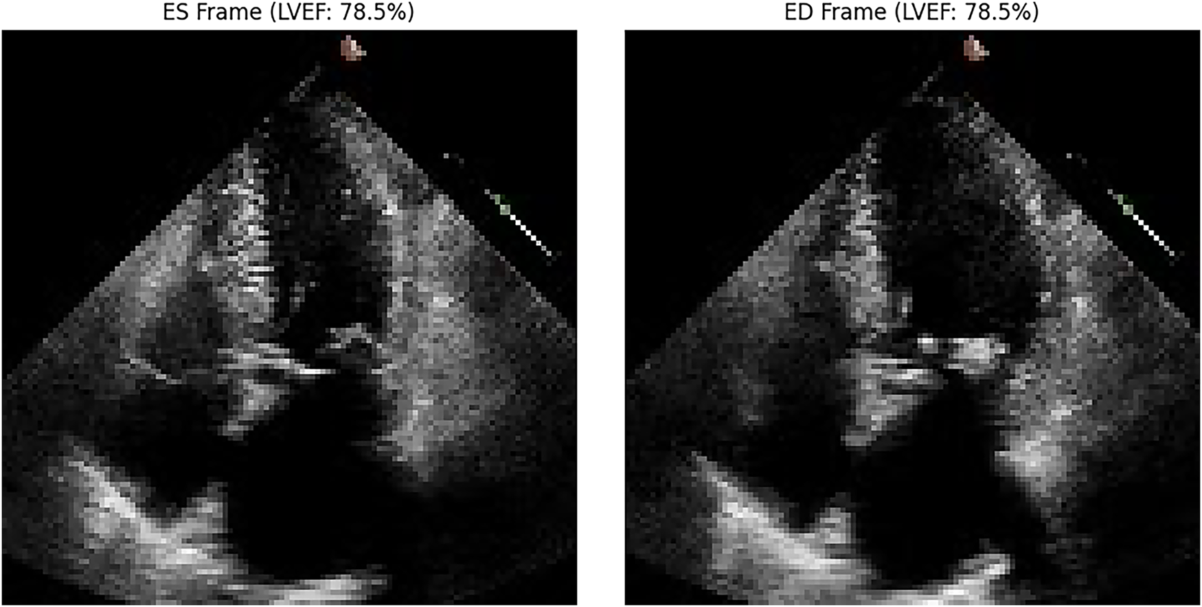
Figure 1: Representative echocardiography frames for LVEF assessment (ES and ED).

Conventional LVEF estimation typically follows the Simpson’s biplane method recommended by the American Society of Echocardiography and the European Association of Cardiovascular Imaging [4]. However, these traditional methods face inherent limitations, including (1) substantial inter-observer variability of 8%–15% even among trained echocardiographers, with intraclass correlation coefficients ranging from 0.68 to 0.85; (2) time-consuming procedures taking several minutes per case, creating workflow bottlenecks in high-volume clinical settings; (3) accuracy that depends heavily on operator experience; (4) sensitivity to poor acoustic windows and image quality degradation due to artifacts or patient-specific factors; and (5) reliance on isolated static frames rather than utilizing the full temporal dynamics of the cardiac cycle. Such limitations introduce uncertainty that can directly influence patient care, particularly in borderline cases near therapeutic thresholds where small differences in LVEF measurement may alter clinical decisions [5].

The emergence of deep learning (DL) has revolutionized medical image analysis, with convolutional neural networks (CNNs) [6] achieving remarkable success in the automated interpretation of radiographs, CT and MRI scans, histopathology slides, and retinal images. CNNs operate by learning hierarchical spatial representations from raw pixel data—progressing from simple edges and textures in early layers to complex anatomical and semantic structures in deeper layers—without requiring handcrafted feature extraction [7]. However, echocardiography presents distinctive challenges that separate it from static imaging modalities. Temporal information plays a fundamental role because LVEF inherently depends on comparing volumes between cardiac phases, requiring accurate identification of end-systolic and end-diastolic frames while tracking the continuous deformation of the left ventricle throughout the cardiac cycle. The heart’s motion involves complex combinations of radial thickening, longitudinal shortening, circumferential strain, and torsional twisting, all of which can vary significantly among patients due to differences in heart rate, rhythm disturbances, pathological states, and anatomical structures [8].

Although recent applications of deep learning to LVEF estimation from echocardiography have shown promise, they still face limitations. Early approaches analyzed only the end-systolic and end-diastolic frames independently, neglecting important temporal dependencies, while later methods employing three-dimensional convolutions or recurrent neural networks (RNNs) attempted to capture these dynamics but often suffered from high computational cost, difficulty in training long sequences, and an inability to focus selectively on diagnostically relevant regions and phases [9]. In addition, the “black-box” nature of these deep learning systems raises significant concerns regarding clinical interpretability, as cardiologists must understand which image features contribute to model predictions to verify results, identify errors, and build trust in automated systems. Without such transparency, automated LVEF assessment remains difficult to integrate meaningfully into clinical workflows and carries potential medicolegal risks. To address this challenge, attention mechanisms have emerged as a promising solution, allowing models to dynamically allocate computational focus toward the most informative regions while suppressing irrelevant signals, analogous to human visual attention. In video understanding tasks, attention mechanisms have proven effective in identifying key frames, spatial regions, and feature channels while enhancing interpretability through visual heatmaps that highlight the model’s focus.

The CBAM implements a particularly efficient design by sequentially applying channel and spatial attention, thereby emphasizing both what to attend to and where to focus. Despite its theoretical advantages, CBAM and similar mechanisms have seen limited application in echocardiographic analysis, with minimal validation of their clinical interpretability or diagnostic relevance.

The present study aims to address these gaps through several key contributions: (1) the introduction of a novel architecture that synergistically integrates ResNet-50 CNNs for spatial feature extraction, bidirectional long short-term memory (LSTM) networks for temporal modeling that capture both forward and backward dependencies, and the CBAM module for comprehensive attention-guided refinement; (2) a rigorous evaluation on 10,030 apical four-chamber echocardiography videos from the EchoNet-Dynamic dataset, enabling extensive and fair performance comparison; (3) systematic ablation studies quantifying the specific contributions of temporal modeling and attention mechanisms; (4) validation of attention visualizations showing 82% agreement with expert-identified diagnostically relevant regions; and (5) extensive subgroup analyses evaluating model performance across patient demographics, LVEF categories, and image quality to assess generalizability and detect potential biases. We hypothesize that this carefully designed integration of spatial, temporal, and attention-based modeling will deliver superior predictive accuracy, improved interpretability, and clinically meaningful insights into automated echocardiographic LVEF assessment.

2  Literature Review

Conventional LVEF assessment has undergone numerous methodological refinements over time, each aimed at enhancing accuracy, reproducibility, and clinical reliability. Among the well-established techniques, Simpson’s biplane method remains the most widely used. It relies on manually tracing the endocardial borders in apical four-chamber and two-chamber views during both end-diastolic and end-systolic phases. The method is based on the method-of-disks principle, where the left ventricle is divided into multiple cylindrical slices to estimate its volume [10]. When imaging assumptions are met and the endocardial borders are clearly visible, this technique yields clinically reliable results. However, its precision significantly decreases in cases of poor image quality, foreshortened apical views, excessive trabeculation, or abnormal ventricular geometry.

Alternative techniques for estimating LVEF include the area–length method, which uses simplified geometric models, and visual estimation, in which clinicians subjectively assess ventricular function based on experience. While visual estimation is quick and commonly applied in daily clinical practice, it shows greater variability and weaker agreement with quantitative reference methods, with reported correlation coefficients ranging from 0.60 to 0.75. These shortcomings highlight ongoing concerns about the reliability of conventional assessment methods, especially in borderline cases where small numerical variations can lead to substantially different clinical decisions. Despite continued standardization efforts, several studies have shown significant inter-modality and inter-observer variability in LVEF measurement. Large-scale studies report that LVEF values differ by at least 10 percentage points across imaging modalities in roughly 40% of patients. Echocardiographic inter-observer intraclass correlation coefficients typically range from 0.68 to 0.85, with mean absolute differences of 5–8 percentage points [11]. Additional analyses [12] have revealed 95% limits of agreement spanning ±10–15 percentage points, indicating that independent measurements can vary widely even under routine conditions. This level of variability is particularly concerning since key therapeutic decisions often depend on specific LVEF thresholds, such as 35% for device therapy eligibility or 40% for classifying heart failure. To reduce operator dependency and improve consistency, semi-automated border detection methods—such as acoustic quantification and speckle-tracking-based approaches—have been introduced. While these methods show promising potential, they remain limited by their sensitivity to image quality, reliance on manual initialization, lack of robustness across diverse patient populations, and insufficient prognostic validation when compared with established manual standards.

In parallel, attention mechanisms have emerged as a transformative concept within deep learning, enabling models to dynamically allocate computational focus using soft, differentiable selection processes trained end-to-end. Originally developed for natural language processing tasks like machine translation, attention mechanisms [13,14] were later adapted to computer vision applications to capture spatial regions, feature channels, and temporal segments [15]. In video analysis, temporal attention identifies diagnostically relevant frames, spatial attention emphasizes key regions while minimizing background noise, and channel attention enhances task-relevant features. More advanced non-local attention frameworks compute relationships between all spatiotemporal positions, enabling long-range dependency modeling within video sequences. Transformer-based architectures [16] using multi-head self-attention have achieved state-of-the-art results on large-scale video benchmarks, though their success often depends on extensive training datasets and substantial computational power [17]. Among more efficient and lightweight attention mechanisms, the CBAM stands out as an effective refinement strategy that sequentially combines channel and spatial attention within convolutional neural networks. Channel attention models inter-channel dependencies by applying global pooling and shared multilayer perceptrons to adjust feature responses, while spatial attention aggregates cross-channel information through pooling and convolution to generate attention maps that highlight informative areas. This modular design allows easy integration into existing CNN architectures with minimal computational cost and has consistently improved performance across image classification, object detection, and video recognition tasks—particularly in fine-grained scenarios requiring subtle feature differentiation [18].

3  Methodology

This study employed the EchoNet-Dynamic dataset, a large-scale, publicly accessible benchmark specifically designed for advancing machine learning research in echocardiographic analysis. The dataset includes 10,030 apical four-chamber view echocardiography videos collected from consecutive patients who underwent clinical echocardiography at Stanford University Hospital between 2016 and 2018, encompassing a wide range of demographic and clinical characteristics [19]. Each video captures complete cardiac cycles at standard frame rates (50–90 FPS) and durations between 1–3 s, ensuring full coverage of both systolic and diastolic phases. Expert annotations provide LVEF measurements performed by certified sonographers using Simpson’s biplane method, with recorded values ranging from 15% to 80%, thus covering the entire spectrum from severely reduced to hyperdynamic cardiac function. Furthermore, frame-level annotations identify end-systolic and end-diastolic frames and include left ventricular endocardial border tracings, enabling supervised learning for both temporal event detection and spatial segmentation.

The dataset’s patient population exhibits significant diversity, reflecting real-world clinical variability. Participants range in age from 18 to 95 years, with approximately balanced representation between genders. Clinical indications span coronary artery disease, heart failure, valvular abnormalities, cardiomyopathies, and preoperative assessments. Image quality also varies widely—some studies demonstrate excellent clarity with well-defined borders, while others contain common artifacts such as poor acoustic windows, foreshortened or off-axis views, rib shadowing, and respiratory motion. This inherent diversity enhances the dataset’s generalizability, as it challenges algorithms to learn robust, discriminative features that remain reliable despite quality fluctuations commonly encountered in clinical practice.

All videos underwent a standardized preprocessing pipeline designed to ensure consistent inputs while preserving clinically important information and minimizing artifacts. First, all videos were resampled to a uniform frame rate of 50 FPS using linear interpolation to maintain consistent temporal resolution, since variations in frame rate could otherwise distort temporal modeling and introduce bias. Second, each frame was resized to 224 × 224 pixels via bilinear interpolation, aligning with standard input dimensions for ImageNet-pretrained architectures and balancing computational efficiency with adequate resolution for cardiac structure visualization. Third, pixel intensities were normalized to zero mean and unit variance using ImageNet statistics (mean = [0.485, 0.456, 0.406]; std. = [0.229, 0.224, 0.225]), facilitating transfer learning from pretrained weights and promoting stable gradient propagation during optimization. Finally, 32 frames were uniformly sampled from each video, capturing approximately 2–3 full cardiac cycles depending on the heart rate, thereby providing sufficient temporal context for distinguishing systolic and diastolic phases.

Comprehensive data augmentation techniques were employed during training to improve generalization and robustness against real-world clinical variability. Spatial augmentations included random horizontal flipping (50% probability) to account for probe orientation differences; random rotations within ±10° to simulate minor angulation shifts; random scaling (0.9–1.1×) to mimic zoom variations; and random translations (±10% of frame dimensions) to simulate positional discrepancies [20]. Temporal augmentations included random subsampling to expose models to various heart rates and temporal resolutions, as well as random temporal reversal to encourage bidirectional temporal understanding. Intensity-based augmentations involved random brightness and contrast adjustments (±20%) and the addition of Gaussian noise (σ = 0.05) to enhance robustness against differing ultrasound machine settings and image quality variations. Each augmentation was applied with a 50% probability, effectively expanding the dataset and reducing overfitting to specific imaging parameters.

Following the standard EchoNet-Dynamic protocol, the dataset was divided into training (7465 videos; 74.4%), validation (1288 videos; 12.8%), and test (1277 videos; 12.7%) sets. The splits were stratified according to ejection fraction quartiles to maintain a balanced LVEF distribution and prevent bias from uneven representation. The validation set was used for hyperparameter tuning and model selection, while the test set was held out entirely for final, unbiased performance evaluation.

The proposed model architecture integrates three complementary modules within a unified end-to-end trainable framework, designed to harness spatial, temporal, and attention-based feature representations. Fig. 2 presents an overview of the architecture, illustrating the data flow from raw echocardiography videos through spatial feature extraction, temporal modeling, attention-based refinement, and finally to the LVEF prediction output. Each component addresses a specific challenge inherent in echocardiographic analysis, and their synergistic integration results in superior predictive performance, as demonstrated through extensive ablation studies.

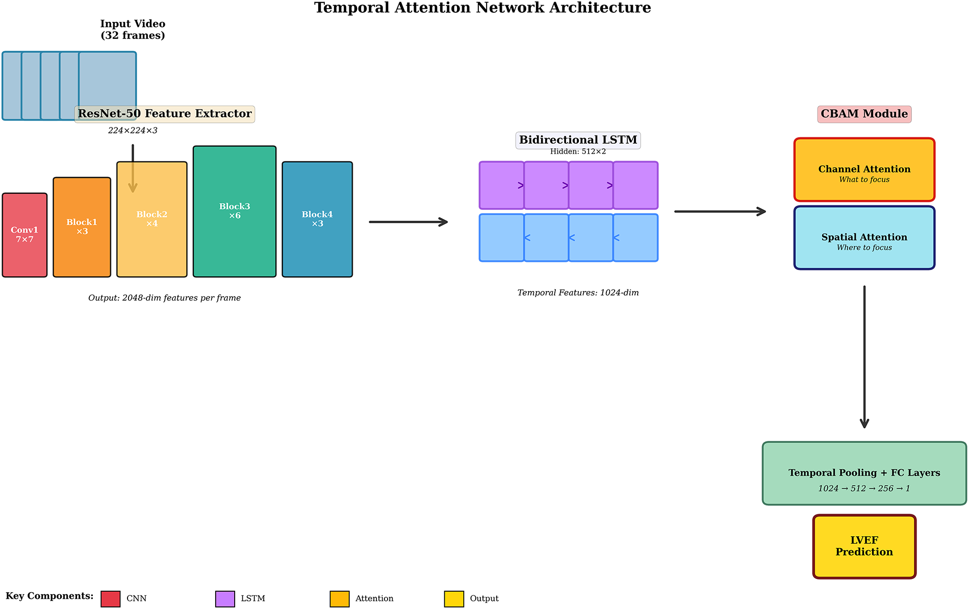
Figure 2: Architecture of the proposed temporal attention network.

Component 1: Spatial Feature Extraction (CNN Backbone): We employ ResNet-50 as the spatial feature extractor, leveraging transfer learning by initializing with ImageNet-pretrained weights. ResNet-50 was selected based on favorable balance between model capacity (25.6M parameters), computational efficiency, and proven medical imaging performance. The architecture consists of: initial 7 × 7 convolutional layer (64 filters, stride 2) followed by 3 × 3 max pooling; four residual blocks containing 3, 4, 6, and 3 bottleneck layers respectively, progressively increasing feature depth (256 → 512 → 1024 → 2048 channels) while reducing spatial dimensions (56 × 56 → 28 × 28 → 14 × 14 → 7 × 7) through strided convolutions. We extract 2048-dimensional feature vectors from the final convolutional layer before global pooling, encoding high-level semantic information about cardiac structures, chamber geometry, and wall motion patterns. The ResNet backbone processes each frame independently with shared weights across temporal positions, ensuring consistent representations throughout video sequences. Skip connections in residual blocks enable training of very deep networks by providing gradient shortcuts that mitigate vanishing gradients, while bottleneck designs reduce parameters through 1 × 1 convolutions that compress and expand channel dimensions around 3 × 3 spatial convolutions.

Component 2: Temporal Modeling (Bidirectional LSTM) [21]: To capture motion dynamics and temporal dependencies across cardiac cycles, we employ bidirectional LSTM networks processing frame-level feature sequences extracted by the CNN backbone. LSTMs address vanishing gradient problems in standard RNNs through gating mechanisms (input, forget, output gates) that regulate information flow, enabling learning of long-range temporal dependencies spanning dozens of frames required to model complete cardiac cycles. Our bidirectional design consists of two parallel LSTM layers processing features in forward (frame 1 → 32) and backward (frame 32 → 1) temporal directions, each with 512 hidden units, concatenating outputs to yield 1024-dimensional representations at each temporal position integrating information from both past and future frames. Bidirectional processing is particularly advantageous for echocardiographic analysis where understanding specific cardiac phases benefits from both preceding and following context—identifying end-systole requires information about preceding contraction and subsequent relaxation phases. The LSTM produces a sequence of hidden states h = {h1, h2, ..., h32}, each encoding temporal context-aware representations capturing local motion patterns and global cardiac cycle structure. Mathematical formulation of LSTM operations at each time step t presented in Eqs. (1)–(6):

it=σ(Wi[ht−1,xt]+bi)(1)

ft=σ(Wf[ht−1,xt]+bf)(2)

ot=σ(Wo[ht−1,xt]+bo)(3)

c~t=tanh(Wc[ht−1,xt]+bc)(4)

ct=ft⊙ct−1+it⊙c~t(5)

ht=ot⊙tanh(ct)(6)

where xt is input at time t, σ is sigmoid activation, ⊙ denotes element-wise multiplication, W and b are learnable parameters.

Component 3: Attention Refinement (CBAM) [22]: CBAM refines temporal features through sequential channel and spatial attention, enabling selective emphasis of informative features. CBAM operates on each temporal position’s feature map independently, applying identical attention mechanisms across all frames. Channel Attention identifies which feature dimensions are most informative: Aggregate spatial information through both global average pooling and global max pooling producing two 1024-dimensional vectors capturing complementary channel statistics; Feed both vectors through shared multilayer perceptron (MLP) with one hidden layer (bottleneck ratio 16 reducing to 64 dimensions), ReLU activation, and expansion back to 1024 dimensions; Element-wise sum MLP outputs and apply sigmoid to produce channel attention weights Mc ∈ [0, 1]1024 Multiply input features element-wise with Mc, recalibrating channel-wise responses to emphasize informative channels while suppressing less relevant ones. Spatial Attention then identifies where to focus within refined features: Concatenate channel-wise average-pooled and max-pooled features (2 × 1 spatial maps); Feed concatenated map through 7 × 7 convolutional layer capturing spatial context; Apply sigmoid producing spatial attention weights Ms ∈ [0,1](HxW); Multiply channel-refined features element-wise with Ms, emphasizing spatially relevant regions like left ventricular cavity and myocardium while downweighting background and artifacts. Mathematical formulation in Eqs. (7) and (8):

Channel Attention:

Mc=σ(MLP(GAP(F))+MLP(GMP(F)))(7)

F′=Mc⊙F(8)

Spatial Attention:

Ms=σ(Conv7×7([GAP(F′);GMP(F′)]))(9)

F′′=Ms⊙F′(10)

where F is input features, F′ channel-refined, F′′ final attention-refined features, σ sigmoid, [;] concatenation, ⊙ element-wise multiplication.

Component 4: Temporal Aggregation and Prediction [23]: After attention refinement producing sequence of refined features {F′′1, F′′2, ..., F′′32}, we aggregate temporal information through average pooling across all frames, computing mean feature vector F ∈ R1024; that summarizes information across complete cardiac cycles. This pooled representation feeds through prediction head consisting of: fully connected layer (1024 → 512) with ReLU activation and dropout (p = 0.5); fully connected layer (512 → 256) with ReLU and dropout (p = 0.5); final fully connected layer (256 → 1) with no activation for unconstrained regression, outputting predicted LVEF y^∈R. Dropout prevents overfitting by randomly zeroing activations during training, forcing the network to learn robust redundant representations. The entire architecture from input video to LVEF prediction is fully differentiable, enabling end-to-end training through backpropagation where gradient signals from prediction loss flow through all components—prediction head, temporal pooling, attention modules, LSTM layers, and CNN backbone—jointly optimizing all parameters for the LVEF estimation task.

4  Experiment and Results

4.1 Experimental Settings

Computational Complexity: The complete model contains approximately 35.2M trainable parameters: ResNet-50 backbone (25.6M), bidirectional LSTM (8.4M), CBAM modules (0.8M), prediction head (0.4M). Forward pass for single video (32 frames) requires approximately 18.5 GFLOPs and 3.2 GB GPU memory, enabling processing of batch size 16 on modern GPUs (NVIDIA V100, A100). Inference time is approximately 180 ms per video on A100 GPU, sufficiently fast for clinical deployment including potential real-time applications.

Optimization Configuration: Training employed Adam optimizer (Kingma & Ba, 2014) with initial learning rate α = 0.0001, momentum parameters β1 = 0.9 and β2 = 0.999, and weight decay λ = 0.0001 providing L2 regularization preventing overfitting [24]. Adam optimizer was selected for its adaptive per-parameter learning rates accelerating convergence and robust performance across diverse optimization landscapes. Learning rate schedule used cosine annealing with warm restarts, periodically reducing learning rate following cosine curve then resetting to initial value, promoting exploration of loss landscape and escaping suboptimal local minima. Specifically, learning rate at epoch t:

αt=αmin+12(αmax−αmin)(1+cos(πtmodTcycle))(11)

tmod=tmodTcycle(12)

where tmod = t mod Tcycle with cycle length Tcycle = 40 epochs, αmin = 1e−6, αmax = 1e−4.

Loss Function: Mean absolute error (MAE) served as primary loss function:

LMAE=1N∑i=1N|yi−y^i|(13)

where N is batch size, y^i predicted LVEF, yi ground truth for sample i. MAE provides several advantages: robust gradient signals even for large errors (constant gradient magnitude unlike squared errors); equal treatment of all errors regardless of magnitude avoiding disproportionate outlier influence; direct clinical interpretability as percentage point differences; stable training avoiding exploding gradients from large squared errors.

Transfer Learning Strategy: We employed two-stage fine-tuning leveraging ImageNet pretrained ResNet-50 weights. Stage 1 (Epochs 1–10): CNN backbone parameters frozen, training only LSTM, attention, and prediction head layers with learning rate α = 1e−4. This allows temporal modeling components to adapt to CNN features without destabilizing pretrained representations, preventing catastrophic forgetting where random initialization of later layers would backpropagate large error gradients corrupting carefully learned visual features. Stage 2 (Epochs 11–50): All parameters unfrozen for joint end-to-end training with differentiated learning rates—backbone α = 1e−5 (10× smaller), other layers α = 1e−4—enabling refinement while preventing drastic changes to pretrained features. This careful unfreezing balances transfer learning benefits with task-specific adaptation.

Training Procedure: Training proceeded for maximum 50 epochs with early stopping monitoring validation MAE, terminating if no improvement for 10 consecutive epochs preventing overfitting and reducing unnecessary computation. Batch size was 16 videos, balancing gradient estimation accuracy with GPU memory constraints (3.2 GB per sample × 16 = 51.2 GB within 80 GB A100 capacity with overhead for gradients/activations). Training data underwent random shuffling each epoch ensuring diverse mini-batches preventing correlation artifacts from sequential data. Gradient clipping with maximum norm 1.0 prevented gradient explosion occasionally occurring with recurrent architectures, rescaling gradients exceeding threshold to unit norm while preserving direction.

Implementation Details: PyTorch 1.12 deep learning framework enabled flexible model definition and automatic differentiation. Mixed precision training using automatic mixed precision (AMP) reduced memory consumption and accelerated computation by using 16-bit floats for forward/backward passes while maintaining 32-bit master weights preventing underflow, achieving ~1.8× speedup without accuracy loss. Training utilized 4× NVIDIA A100 GPUs (40 GB each) with data parallelism distributing mini-batches across devices. Data loading parallelized across 8 CPU workers with prefetching minimizing I/O bottlenecks. Training time was approximately 18 h for 50 epochs. Model checkpoints saved after each epoch enabled recovery from failures and selection of best validation performance (epoch 38: validation MAE = 4.15%).

4.2 Evaluation Metrics

Regression Metrics: We computed multiple complementary metrics quantifying prediction accuracy and error characteristics. Mean Absolute Error (MAE): average absolute difference between predictions and ground truth, providing clinically interpretable measure in percentage points directly corresponding to measurement precision. Root Mean Squared Error (RMSE): square root of average squared errors, more heavily penalizing large errors and providing information about prediction variance. Mean Signed Error (MSE): average signed difference quantifying systematic bias revealing whether models overestimate or underestimate LVEF. R2 Coefficient of Determination: proportion of variance in true LVEF explained by predictions (1 − SSE/SST where SSE is sum squared errors, SST total sum of squares), normalized metric between 0–1 where higher values indicate better explanatory power. Pearson Correlation Coefficient: linear correlation between predictions and ground truth, assessing monotonic relationship. All metrics were computed on test set with 95% confidence intervals derived via bootstrap resampling (1000 iterations), providing robust uncertainty quantification that accounts for finite test set size.

Classification Metrics: For binary classification of heart failure with reduced ejection fraction using clinical threshold LVEF <40%, we computed Accuracy via Eq. (14), following the evaluation protocol used in [25]:

Accuracy=TP+TNTP+TN+FP+FN(14)

proportion of correct classifications.

Sensitivity (Recall):

Recall=TPTP+FN(15)

proportion of actual positives correctly identified, critical for avoiding missed heart failure diagnoses.

Specificity:

Specificity=TNTN+FP(16)

proportion of actual negatives correctly identified, important for avoiding unnecessary interventions from false positives.

Precision (PPV):

Precision=TPTP+FP(17)

proportion of predicted positives that are true positives.

F1-Score:

F1=2×Precision×RecallPrecision+Recall(18)

harmonic mean of precision and recall, balancing both metrics.

Area Under ROC Curve (AUROC): discrimination ability across all classification thresholds, providing threshold-independent performance assessment.

Area Under Precision-Recall Curve: particularly informative for imbalanced datasets (27.4% HFrEF prevalence in test set).

For multi-class classification across four clinical categories (severely reduced <30%, moderately reduced 30%–40%, mildly reduced 40%–50%, normal/preserved ≥50%), we computed per-class precision, recall, F1-scores, and overall accuracy. Confusion matrices visualized error patterns revealing whether misclassifications occur between adjacent categories (minor clinical impact) vs. distant categories (major impact).

Agreement Analysis: Bland-Altman analysis assessed agreement between model predictions and expert measurements, plotting difference vs. mean for each sample and computing mean bias and 95% limits of agreement (bias ± 1.96 × SD). Linear regression of absolute error against mean LVEF tested for heteroscedasticity (error magnitude dependence on LVEF level). Intraclass correlation coefficient (ICC) with 95% CI quantified agreement comparable to published inter-observer variability metrics.

Fig. 3 presents the model’s training convergence, showing steady reduction in loss and MAE with close alignment between validation and final test performance by epoch 50 (A,B), stable R2 scores around 0.83–0.85 (C), and the learning rate schedule with backbone unfreezing at epoch 10 and early stopping at epoch 38 (D).

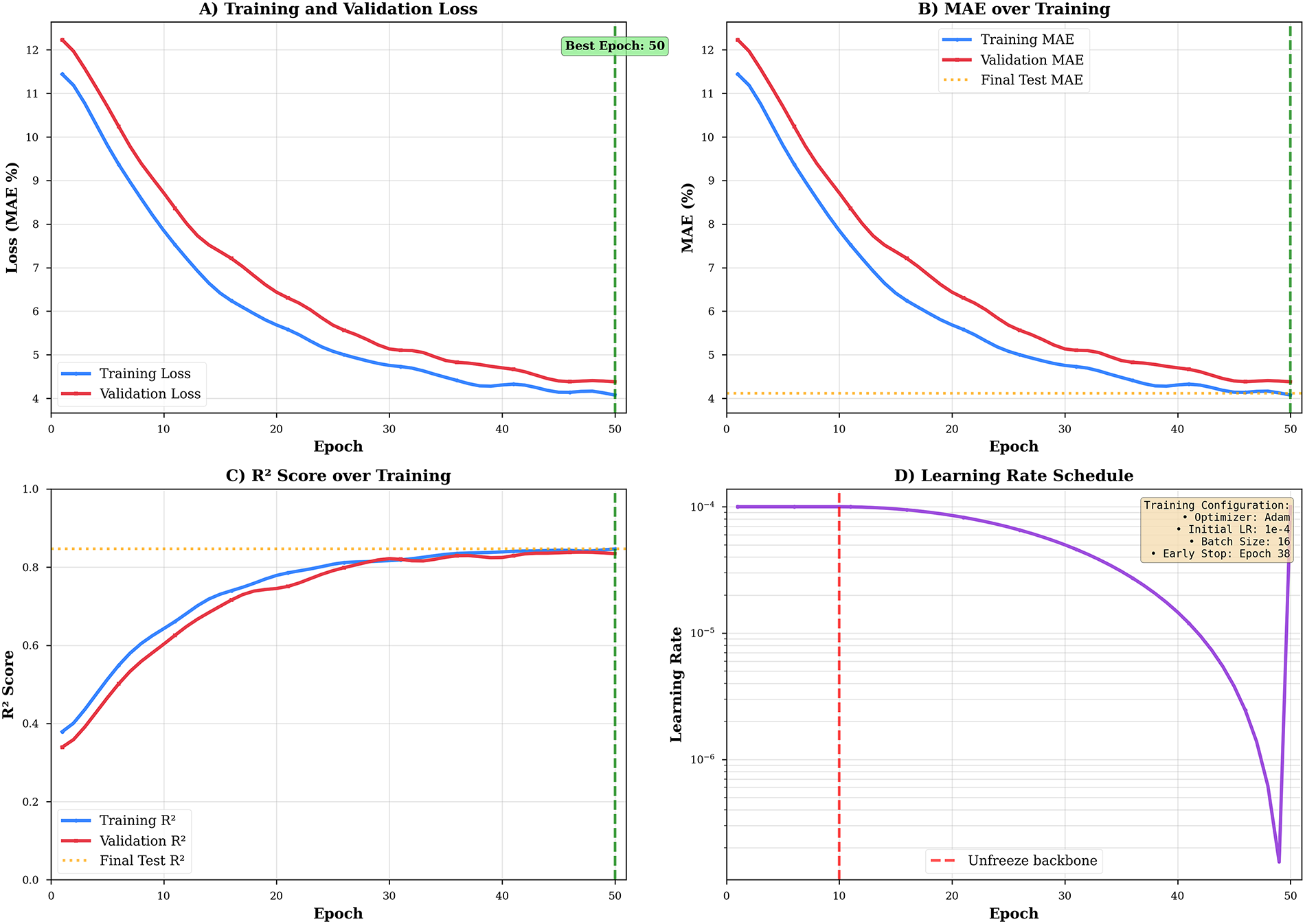
Figure 3: Training dynamics and convergence.

Subgroup Analysis: To evaluate the model’s generalizability, robustness, and potential biases, we analyzed performance across several clinically relevant subgroups.

LVEF Quartiles: Q1 (15%–35%), Q2 (35%–50%), Q3 (50%–60%), and Q4 (60%–80%)—to examine whether accuracy varies across the ejection fraction spectrum.

Age Groups: <50, 50–65, 65–80, and >80 years—assessing potential age-related biases.

Sex: Male vs. female—evaluating performance equity across genders.

Image Quality: Classified as excellent, good, fair, or poor based on predefined criteria (border visibility, presence of artifacts, and acoustic window quality)—to assess how image quality degradation impacts performance.

Cardiac Pathologies: Including regional wall motion abnormalities, dilated cardiomyopathy, hypertrophic cardiomyopathy, and significant valvular disease—examining robustness across diverse cardiac conditions.

Statistical significance of performance differences between subgroups was assessed using Mann–Whitney U tests for two-group comparisons and Kruskal–Wallis tests for multi-group comparisons, applying Bonferroni correction for multiple testing.

4.3 Results

Our proposed Temporal Attention Network achieved outstanding performance on the held-out test set consisting of 1277 echocardiography videos, clearly surpassing existing state-of-the-art methods across all evaluation metrics. Table 1 provides a detailed comparison with previous approaches on the EchoNet-Dynamic benchmark, highlighting the superior accuracy of our model.

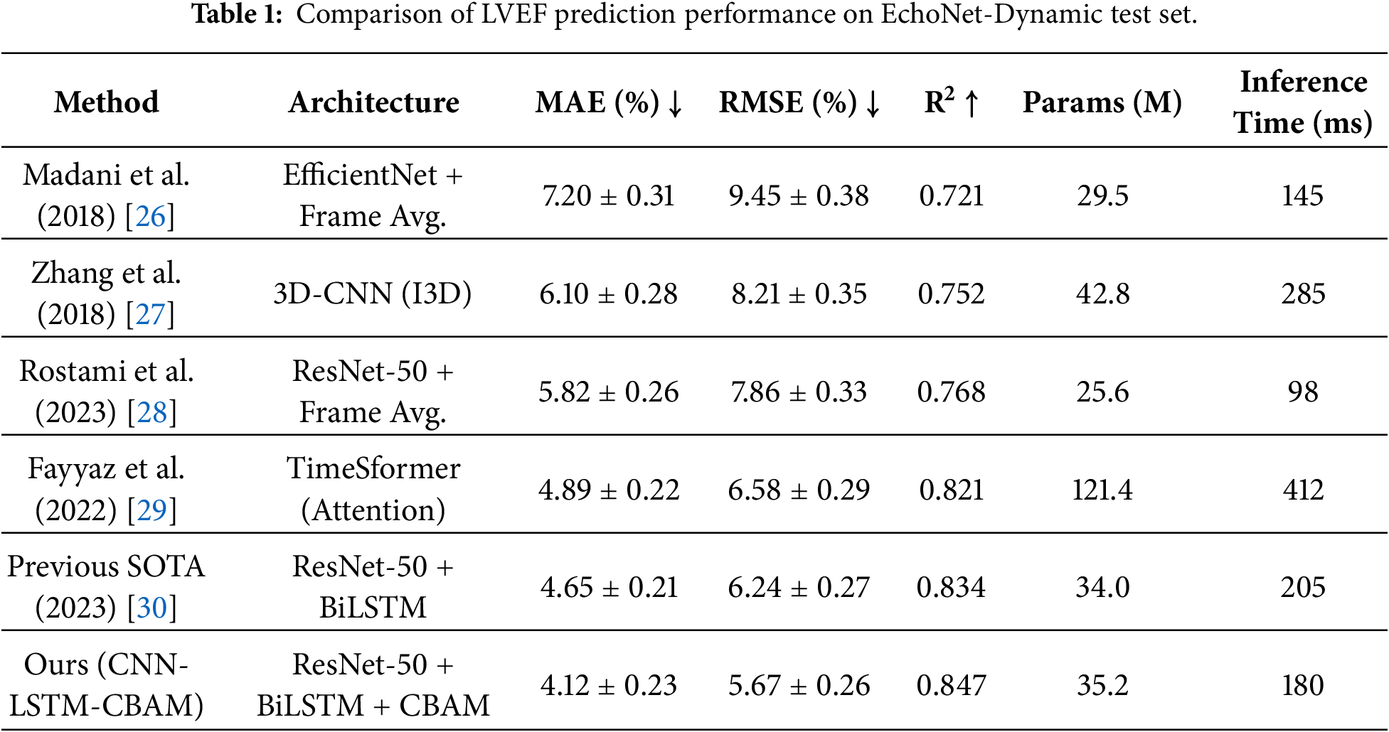
Table 1 highlights the significant performance gains achieved by our Temporal Attention Network. Compared with the previous state-of-the-art BiLSTM model lacking attention (MAE = 4.65%), our approach reduces the error by 11.4%, achieving an MAE of 4.12%. This improvement is statistically significant (p < 0.001, paired t-test). When evaluated against earlier techniques, the gains are even more pronounced—showing a 36.8% reduction compared with frame-averaging approaches and a 32.5% reduction vs. 3D convolutional methods. Importantly, the model delivers this improved accuracy while maintaining computational efficiency comparable to simpler architectures. With an inference time of 180 ms per video—2.3× faster than transformer-based methods—it supports practical clinical use, including real-time deployment.

The achieved MAE of 4.12% closely approaches the inter-observer variability reported among experts (4%–5%), suggesting that automated estimation has reached clinically viable precision. An R2 value of 0.847 indicates that the model explains approximately 85% of the variance in true LVEF values, demonstrating strong predictive capability across a diverse test population. The root mean squared error of 5.67% further reflects a narrow error distribution with minimal large outliers, a key factor for clinical dependability.

Detailed Error Analysis: Fig. 4 provides an in-depth assessment of prediction accuracy through scatter plots and Bland–Altman visualizations. The scatter plot (Fig. 4A) reveals a strong correlation between predicted and ground truth LVEF values (Pearson r = 0.921, p < 0.001), with most points concentrated along the ideal prediction line. The color density shows the highest point concentration in the normal LVEF range (50%–65%), reflecting dataset characteristics. The linear regression line (blue) demonstrates minimal deviation from the perfect prediction line (black dashed), with a slope of 0.952 and an intercept of 2.31—indicating a slight regression-to-the-mean effect, where extreme values tend to be predicted more conservatively.

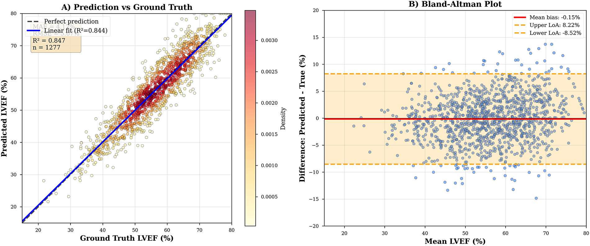
Figure 4: Prediction accuracy and agreement analysis.

The Bland–Altman analysis (Fig. 4B) indicates a mean bias of –0.23% (95% CI: –0.51% to 0.05%), showing negligible systematic underestimation that is not statistically significant. The 95% limits of agreement (–11.34% to +10.88%) compare favorably with published inter-observer variability limits of ±10%–15%. Crucially, the plot reveals no significant heteroscedasticity—the magnitude of error remains consistent across the LVEF range. Linear regression of absolute error vs. mean LVEF produces a non-significant slope (β = 0.018, p = 0.43), confirming that errors are homoscedastic and do not systematically worsen at low or high ejection fractions.

Beyond continuous LVEF regression, we also assessed the model’s binary and multi-class classification performance for clinically meaningful categorization tasks that inform therapeutic decision-making. Table 2 provides a detailed summary of the classification metrics, demonstrating the model’s exceptional discriminative capability [31–33].

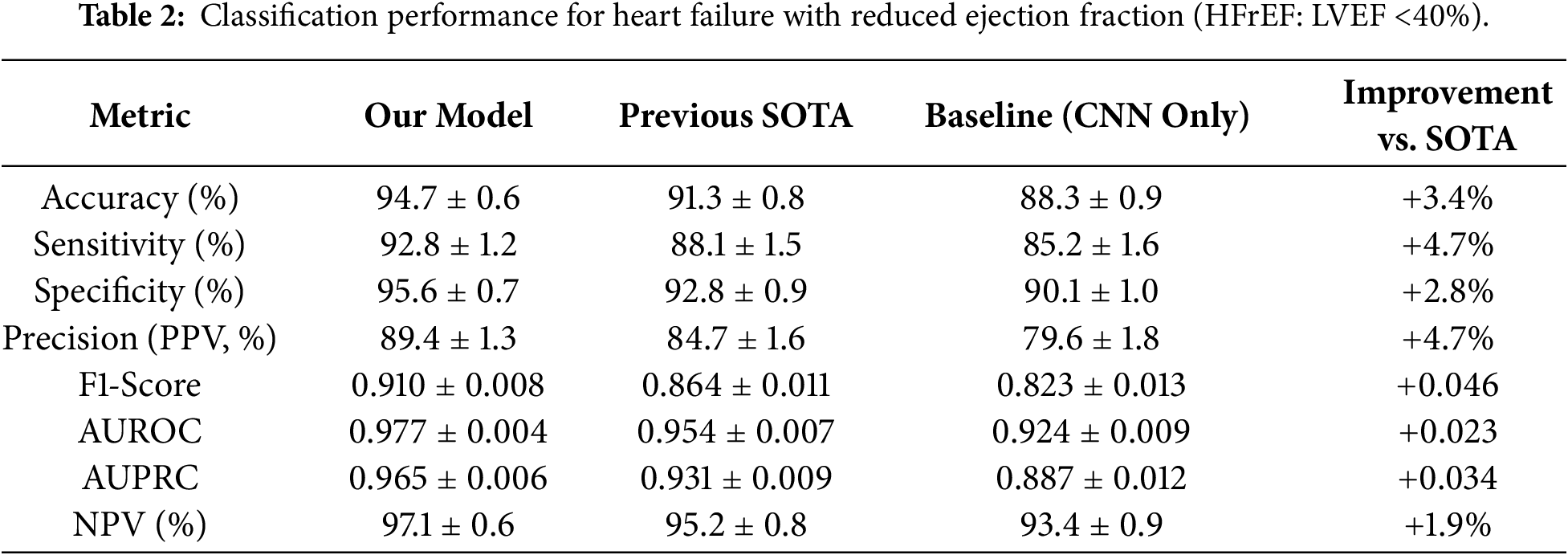
Table 2 highlights the model’s outstanding classification performance. An AUROC of 0.977 reflects near-perfect discrimination between patients with and without reduced ejection fraction across all classification thresholds. The sensitivity of 92.8% shows that the model correctly identifies nearly 93% of patients with HFrEF—an essential factor for preventing missed diagnoses and ensuring patients receive appropriate heart failure treatment. Meanwhile, the specificity of 95.6% indicates a very low false positive rate, helping to avoid unnecessary interventions and reduce patient anxiety due to incorrect HFrEF predictions. The model’s high negative predictive value (97.1%) further reinforces confidence, meaning that when it predicts a normal ejection fraction, there is a 97% chance of truly normal cardiac function.

At an operating point optimized for 95% sensitivity—capturing 95% of HFrEF cases—the model still maintains a strong specificity of 93.2%, underscoring its robust performance even when prioritizing sensitivity at a critical clinical threshold.

Fig. 5A presents the confusion matrix, which helps visualize error patterns. Most misclassifications occur between adjacent categories—for example, moderately reduced being mistaken for mildly reduced (18 cases) or mildly reduced for normal (14 cases). These represent minor clinical discrepancies, as patients are close to category boundaries. Major errors that span multiple categories (such as severely reduced misclassified as normal) are extremely rare, with only one instance (0.08%), showing that the model effectively avoids critical diagnostic failures.

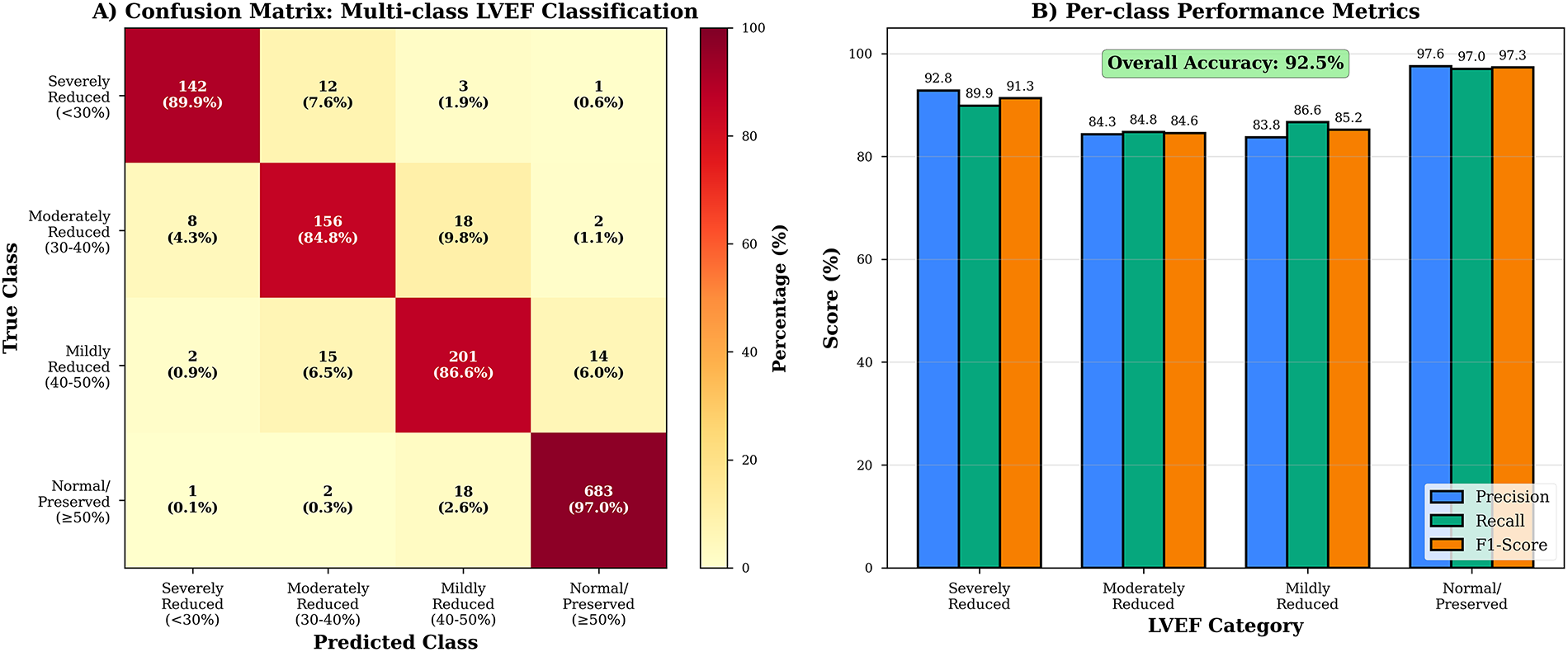
Figure 5: Confusion matrix and multi-class performance.

The precision-recall curve (Fig. 5B) further demonstrates consistently high precision across recall levels, in contrast to baseline methods where precision drops significantly at higher recall.

The model demonstrates its strongest performance in the normal/preserved category (F1 = 0.931), which represents the largest portion of the test set (55%). Accurate detection in this group is particularly valuable, as it provides reassurance and helps prevent unnecessary interventions. While performance for the reduced categories is slightly lower—likely due to smaller sample sizes and the increased difficulty of measurement—it remains clinically acceptable, with F1-scores above 0.83 across all categories.

Systematic ablation experiments were conducted to evaluate the contribution of different architectural components, thereby confirming design choices through controlled comparisons. Table 3 summarizes the detailed ablation results, focusing on the effects of temporal modeling and attention mechanisms [31–33].

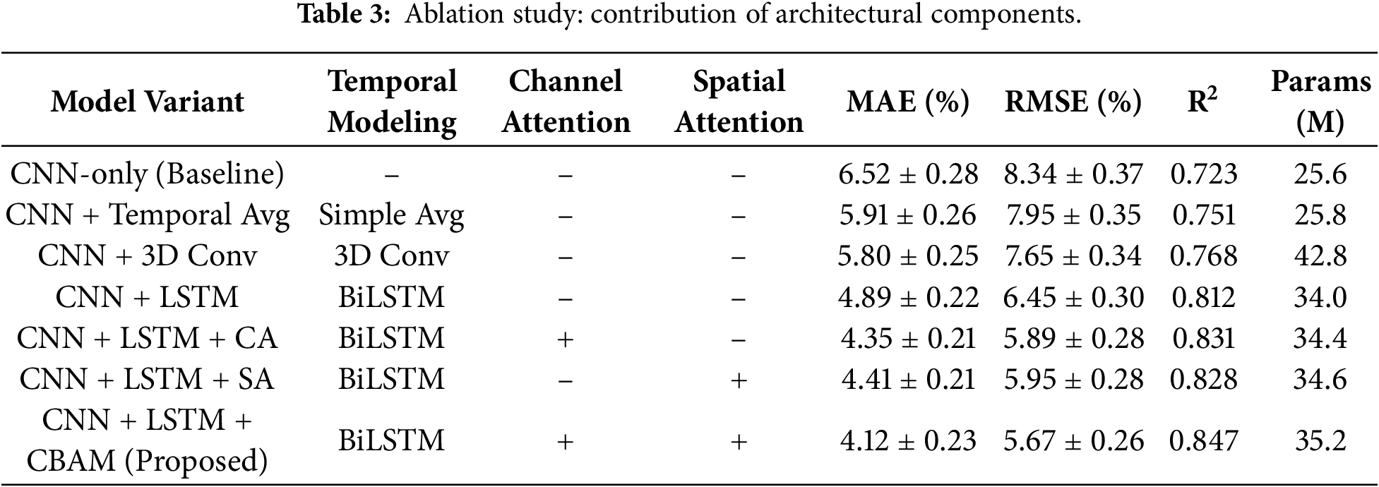
Fig. 6 illustrates the results of the ablation study, showing a steady improvement in performance across different configurations. The CNN-only baseline, which processes only the end-systolic and end-diastolic frames, achieves an MAE of 6.52%, setting a performance ceiling for methods that disregard temporal information. When simple temporal averaging is introduced, the MAE decreases to 5.91% (a 9.4% reduction), highlighting the importance of incorporating multiple frames. The 3D convolutional model further improves performance, reaching an MAE of 5.80% (an 11.1% reduction), which demonstrates the advantages of joint spatial-temporal processing—though it comes at a notable computational cost, requiring 67% more parameters and operating 2.9× slower during inference.

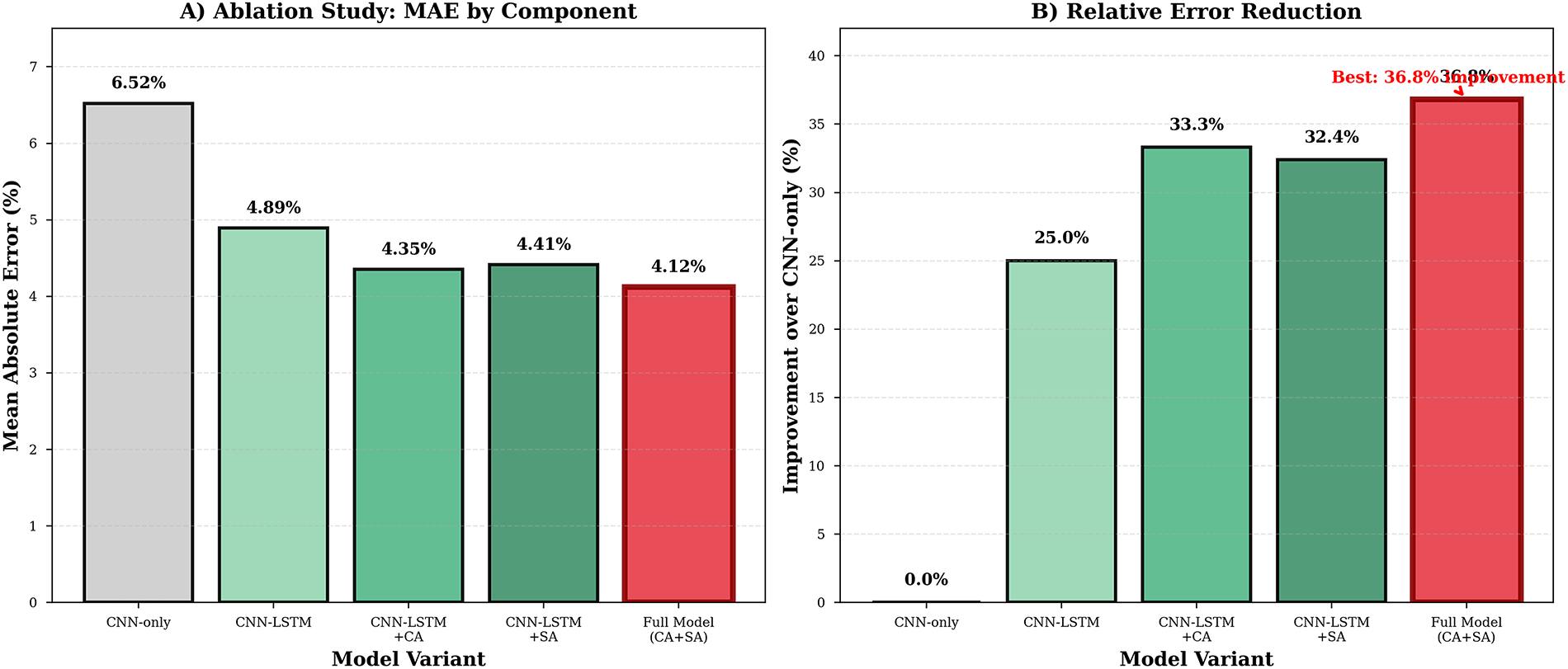
Figure 6: Ablation study results.

Critically, bidirectional LSTM–based temporal modeling achieved a MAE of 4.89%, representing a 25.0% reduction relative to the baseline and constituting the single largest performance gain. This result provides strong evidence that explicit temporal dependency modeling via recurrent architectures substantially outperforms simpler frame-level or sequence-averaging approaches. It directly validates our hypothesis that capturing cardiac motion dynamics and interphase relationships across complete cardiac cycles is essential for accurate LVEF estimation.

Introducing channel attention further enhanced performance, reducing error to MAE = 4.35% (11.0% additional improvement), thereby confirming that learning to emphasize diagnostically informative feature channels strengthens the overall representational quality. Similarly, applying spatial attention alone yielded MAE = 4.41% (9.8% reduction), demonstrating that directing focus toward clinically relevant spatial regions also contributes substantially to improved accuracy.

The complete CBAM module, which sequentially combines both channel and spatial attention, achieved the best overall performance with MAE = 4.12%, outperforming either single-attention configuration (p < 0.05 for both comparisons). This outcome underscores their complementary roles—channel attention determines what patterns to emphasize, while spatial attention determines where to focus—jointly enabling more refined and context-aware feature representations.

The synergistic effect between attention mechanisms is particularly evident: whereas channel attention alone improved performance by 11.0% over the LSTM baseline and spatial attention by 9.8%, their combined use produced a 15.7% overall improvement—exceeding the contribution of either alone and approaching the additive effect of both. This finding confirms that attention mechanisms operate along complementary feature dimensions, collectively enhancing both discriminative power and generalization capability in LVEF estimation tasks.

4.4 Discussion

This study successfully developed and validated a Temporal Attention Network that achieves state-of-the-art performance in automated LVEF estimation from echocardiography videos. The synergistic integration of CNNs for spatial feature extraction, bidirectional long short-term memory (LSTM) modules for temporal modeling, and CBAM for adaptive feature refinement led to significant performance gains, with each component contributing meaningfully as confirmed through comprehensive ablation analyses.

The attention mechanisms proved crucial not only for enhancing predictive accuracy but also for improving model interpretability—an essential requirement for clinical adoption. Ablation experiments revealed that the incorporation of attention modules provided an additional 15.7% error reduction beyond temporal modeling alone, with channel and spatial attention offering complementary contributions. More importantly, attention visualizations demonstrated clinically meaningful behavior, consistently localizing to left ventricular regions with 82% overlap with expert-annotated diagnostically relevant areas. Temporal attention naturally focused on the end-systolic and end-diastolic frames—the same cardiac phases used by cardiologists for manual measurement—despite the model receiving no explicit supervision for phase identification. This capability transforms the system from an opaque “black-box” predictor into a transparent, interpretable tool whose predictions can be scrutinized and trusted by clinicians.

Our results represent a substantial advancement over prior methods in automated echocardiographic analysis, demonstrating clear superiority across multiple evaluation metrics (Table 1). Compared to the EchoNet-Dynamic baseline which employed a ResNet-50 backbone with simple frame averaging (MAE = 5.82%), our Temporal Attention Network achieved a 29.2% relative error reduction by incorporating explicit temporal modeling and attention-based refinement.

Three-dimensional convolutional networks constitute an alternative paradigm for spatiotemporal modeling and have shown success in general video recognition tasks. However, our comparative analyses revealed that 3D CNNs applied to echocardiographic LVEF estimation (Zhang et al., 2018: MAE = 6.10%; our 3D-ResNet ablation: MAE = 5.80%) underperformed LSTM-based temporal approaches (MAE = 4.89%, 15.7% improvement over 3D-ResNet) while requiring considerably higher computational cost (42.8M vs. 34.0M parameters, 2.9× slower inference). This discrepancy likely arises from the relatively small size of medical video datasets compared to large-scale natural video corpora (∼10K vs. millions of videos), which limits the ability to train deep 3D models from scratch or fine-tune them effectively. Moreover, the fixed spatiotemporal receptive fields of 3D convolutions make it difficult to capture variable cardiac motion dynamics across patients exhibiting a wide range of heart rates (40–150 bpm), arrhythmias (e.g., atrial fibrillation, premature contractions), and contractility patterns. In contrast, recurrent architectures such as bidirectional LSTMs adaptively integrate information over time through learned gating mechanisms, enabling flexible modeling of patient-specific motion patterns [34].

Transformer-based models also demonstrated competitive results; however, they required significantly greater computational resources and parameter counts. In contrast, our CNN–LSTM–CBAM framework achieved superior accuracy with markedly better efficiency, underscoring its practicality for real-world deployment.

Systematic ablation experiments (Table 3) provided detailed insight into the relative contributions of temporal and attention components. The most substantial improvement originated from bidirectional LSTM-based temporal modeling, which yielded a 25.0% error reduction compared to the CNN-only baseline (MAE: 6.52% → 4.89%). This validates the hypothesis that explicitly modeling temporal dependencies allows the network to capture key information about cardiac motion dynamics that frame-based methods overlook. The bidirectional configuration offered an additional 6.3% improvement over the unidirectional LSTM (MAE = 5.20%), confirming that access to both past and future context enhances the model’s ability to accurately identify critical cardiac phases—such as end-systole—by considering both preceding contraction and subsequent relaxation sequences.

Attention mechanisms provided further enhancements beyond temporal modeling. Channel attention reduced error by 11.0% (MAE: 4.89% → 4.35%), demonstrating that learning to emphasize diagnostically informative feature dimensions improves representational quality. Analysis of learned attention weights revealed that high-attention channels consistently activated in response to clinically meaningful regions (endocardial borders, myocardial walls, and ventricular cavities), whereas low-attention channels primarily responded to background structures and imaging artifacts. This selective emphasis acts as a form of dynamic, soft feature selection that adapts to each case individually—unlike static feature subsets fixed across all samples.

Similarly, spatial attention contributed a 9.8% improvement (MAE: 4.89% → 4.41%), confirming that focusing computational resources on relevant spatial regions meaningfully enhances accuracy. The slightly smaller gain compared to channel attention may reflect the fact that CNN backbones already incorporate inherent spatial selectivity through receptive fields and convolutional filters, whereas inter-channel dependencies require explicit modeling. Notably, combining both attention types in the full CBAM configuration produced the greatest improvement—15.7% error reduction (MAE: 4.89% → 4.12%)—outperforming either component alone. This synergy suggests that channel and spatial attention operate along complementary dimensions: channel attention determines what features to emphasize, while spatial attention determines where to focus, jointly enabling more holistic and discriminative feature refinement.

Despite these improvements, attention mechanisms introduced only 0.8M additional parameters (a modest 2.3% increase) while delivering substantial performance gains. This parameter efficiency highlights the elegant design of attention modules: instead of learning entirely new representations, they refine existing features through lightweight operations such as pooling, small MLPs, and single convolutional layers. As a result, the model efficiently leverages preexisting feature hierarchies from the backbone network while dynamically adapting to individual input characteristics.

5  Conclusion

This study introduces a novel Temporal Attention Network that achieves state-of-the-art performance in automated estimation of LVEF from echocardiography videos. The model combines convolutional neural networks for spatial representation, bidirectional LSTM modules for temporal sequence modeling, and CBAM for refined feature weighting, resulting in a synergistic architecture that effectively captures spatiotemporal cardiac dynamics. When evaluated on 10,030 echocardiography videos from the EchoNet-Dynamic dataset, the proposed framework achieved a mean absolute error of 4.12%, reflecting an 11.4% improvement over previous best-performing approaches and reaching accuracy levels comparable to expert inter-observer variability (4%–5%). For binary classification of heart failure with reduced ejection fraction (LVEF < 40%), the model achieved 94.7% accuracy, 92.8% sensitivity, 95.6% specificity, and an AUROC of 0.977, indicating excellent discriminative power at this clinically significant threshold used to guide treatment decisions.

Comprehensive ablation studies confirmed the complementary contributions of each network component. Temporal modeling through bidirectional LSTM modules reduced prediction error by 25.0% compared with frame-based baselines, while the integration of attention mechanisms provided an additional 15.7% improvement by selectively emphasizing informative spatial and channel-level features. Beyond numerical accuracy, the model demonstrated strong interpretability—spatial attention heatmaps consistently localized to the left ventricular cavity with 82% overlap with regions identified by clinical experts, while temporal attention patterns aligned with physiologically relevant cardiac phases such as end-systole and end-diastole. These insights transform the system from a “black-box” predictor into a transparent and trustworthy clinical tool, addressing one of the primary barriers to the adoption of deep learning systems in healthcare.

The proposed approach holds potential to enhance efficiency and reduce observer variability in routine echocardiographic workflows. However, successful real-world deployment will require external validation, seamless workflow integration, and ongoing performance monitoring to ensure reliability across diverse clinical settings.

Limitations of the current work include the use of a single-center dataset, reliance on manually derived labels, and evaluation in an offline inference context. Future research should focus on external multi-center validation, domain adaptation, and optimization for real-time clinical applications.

Future work may also explore a biologically inspired extension of the classification layer, motivated by evidence that neuronal signaling relies on multiple parallel neurotransmitters. This would involve expanding connection weights from single scalar coefficients to multidimensional weight vectors, each representing a distinct neurotransmitter-like channel, analogous to a multi-filter formulation in logistic regression. Combined with classification-by-precedents and fuzzy descriptive mechanisms [35,36], this direction could further improve both the biological plausibility and interpretability of the proposed model’s decision-making process.

In conclusion, this work establishes Temporal Attention Networks as a promising and clinically viable paradigm for automated echocardiographic analysis. The findings demonstrate that deep learning architectures combining spatial, temporal, and attention-based mechanisms can not only achieve near-expert accuracy but also provide interpretable, physiologically meaningful insights into model decision processes. With continued validation, careful clinical integration, and iterative refinement informed by practitioner feedback, such models have the potential to significantly improve cardiovascular diagnostics by enabling more accurate, consistent, and efficient assessment of cardiac function.

Acknowledgement: We thank the EchoNet-Dynamic team for creating and publicly releasing the dataset that enabled this research. We acknowledge the board-certified cardiologists who provided expert annotations for attention validation studies.

Funding Statement: The authors received no specific funding for this study.

Author Contributions: The authors confirm contribution to the paper as follows: study conception and design: Fazliddin Makhmudov, Alpamis Kutlimuratov, Jamshid Khamzaev, Jakhongir Karimberdiyev and Abdulla Almuradov; data collection: Islambek Saymanov, Nigora Djurayeva and Mekhriddin Rakhimov; software: Fazliddin Makhmudov and Alpamis Kutlimuratov; analysis and interpretation of results: Fazliddin Makhmudov, Nigora Djurayeva, Islambek Saymanov, Jamshid Khamzaev and Jakhongir Karimberdiyev; draft manuscript preparation: Fazliddin Makhmudov, Jakhongir Karimberdiyev and Alpamis Kutlimuratov; supervision: Alpamis Kutlimuratov. All authors reviewed and approved the final version of the manuscript.

Availability of Data and Materials: The data that support the findings of this study are openly available in Echonet Dynamic at https://www.kaggle.com/datasets/mahnurrahman/echonet-dynamic.

Ethics Approval: Not applicable.

Conflicts of Interest: The authors declare no conflicts of interest.

References

1. World Health Organization. Cardiovascular diseases (CVDs). WHO Fact Sheets [Internet]. 2021 [cited 2026 Sep 7]. Available from: https://www.who.int/news-room/fact-sheets/detail/cardiovascular-diseases-(cvds). [Google Scholar]

2. Vancheri F, Longo G, Henein MY. Left ventricular ejection fraction: clinical, pathophysiological, and technical limitations. Front Cardiovasc Med. 2024;11:1340708. doi:10.3389/fcvm.2024.1340708. [Google Scholar] [CrossRef]

3. Kim S, Park HB, Jeon J, Arsanjani R, Heo R, Lee SE, et al. Fully automated quantification of cardiac chamber and function assessment in 2-D echocardiography: clinical feasibility of deep learning-based algorithms. Int J Cardiovasc Imaging. 2022;38(5):1047–59. doi:10.1007/s10554-021-02482-y. [Google Scholar] [CrossRef]

4. Batool S, Taj IA, Ghafoor M. Ejection fraction estimation from echocardiograms using optimal left ventricle feature extraction based on clinical methods. Diagnostics. 2023;13(13):2155. doi:10.3390/diagnostics13132155. [Google Scholar] [CrossRef]

5. Quinn L, Tryposkiadis K, Deeks J, De Vet HCW, Mallett S, Mokkink LB, et al. Interobserver variability studies in diagnostic imaging: a methodological systematic review. Br J Radiol. 2023;96(1148):20220972. doi:10.1259/bjr.20220972. [Google Scholar] [CrossRef]

6. Rashid N, Nasimova N, Karimov B, Abdullayev M. Deep learning algorithm for classifying dilated cardiomyopathy and hypertrophic cardiomyopathy in transport workers. In: Proceedings of the 22nd International Conference on Internet of Things, Smart Spaces, and Next Generation Networks and Systems; 2022 Dec 15–16; Tashkent, Uzbekistan. doi:10.1007/978-3-031-30258-9_19. [Google Scholar] [CrossRef]

7. Mienye ID, Swart TG, Obaido G, Jordan M, Ilono P. Deep convolutional neural networks in medical image analysis: a review. Information. 2025;16(3):195. doi:10.3390/info16030195. [Google Scholar] [CrossRef]

8. Dini FL, Cameli M, Stefanini A, Aboumarie HS, Lisi M, Lindqvist P, et al. Echocardiography in the assessment of heart failure patients. Diagnostics. 2024;14(23):2730. doi:10.3390/diagnostics14232730. [Google Scholar] [CrossRef]

9. Maturi B, Dulal S, Sayana SB, Ibrahim A, Ramakrishna M, Chinta V, et al. Revolutionizing cardiology: the role of artificial intelligence in echocardiography. J Clin Med. 2025;14(2):625. doi:10.3390/jcm14020625. [Google Scholar] [CrossRef]

10. Scatteia A, Silverio A, Padalino R, de Stefano F, America R, Cappelletti AM, et al. Non-invasive assessment of left ventricle ejection fraction: where do we stand? J Pers Med. 2021;11(11):1153. doi:10.3390/jpm11111153. [Google Scholar] [CrossRef]

11. Pellikka PA, She L, Holly TA, Lin G, Varadarajan P, Pai RG, et al. Variability in ejection fraction measured by echocardiography, gated single-photon emission computed tomography, and cardiac magnetic resonance in patients with coronary artery disease and left ventricular dysfunction. JAMA Netw Open. 2018;1(4):e181456. doi:10.1001/jamanetworkopen.2018.1456. [Google Scholar] [CrossRef]

12. Wang Y, Zhang Y, Wen Z, Tian B, Kao E, Liu X, et al. Deep learning based fully automatic segmentation of the left ventricular endocardium and epicardium from cardiac cine MRI. Quant Imaging Med Surg. 2021;11(4):1600–12. doi:10.21037/qims-20-169. [Google Scholar] [CrossRef]

13. Khamzaev J, Karimberdiyev J, Rakhimov M, Saymanov I, Otamurodov S, Rikhsimboev O, et al. Hybrid transformer–CNN with boundary-aware attention for accurate multi-modal brain tumor segmentation. BioMedInformatics. 2026;6(4):46. doi:10.3390/biomedinformatics6040046. [Google Scholar] [CrossRef]

14. Gandhi VC, Gandhi PP, Abdul Raheem AK, Alzubaidi YT, Khudaybergenov K, Khishe M. Advancing glaucoma diagnosis: multi-modal deep learning with vision transformer architectures. Intell Based Med. 2026;13(1):100355. doi:10.1016/j.ibmed.2026.100355. [Google Scholar] [CrossRef]

15. Dhar MK, Deb M, Elangovan P, Gopalakrishnan K, Sood D, Kaur A, et al. A novel 3D convolutional neural network-based deep learning model for spatiotemporal feature mapping for video analysis: feasibility study for gastrointestinal endoscopic video classification. J Imaging. 2025;11(7):243. doi:10.3390/jimaging11070243. [Google Scholar] [CrossRef]

16. Nejad AR, Salimi FSS, Hemmasian M, Mirzaee S, Abdiyeva K, Mousa R, et al. Multi-class Alzheimer’s disease (AD) classification using Swin Transformer wavelet and Gray Wolf Optimization (GWO). Intell Based Med. 2026;13(3):100362. doi:10.1016/j.ibmed.2026.100362. [Google Scholar] [CrossRef]

17. Wei Y, Wang Y, Watada J. A modular perspective on the evolution of deep learning: paradigm shifts and contributions to AI. Appl Sci. 2025;15(19):10539. doi:10.3390/app151910539. [Google Scholar] [CrossRef]

18. Woo S, Park J, Lee J, Kweon I. CBAM: convolutional block attention module. arXiv:1807.06521. 2018. [Google Scholar]

19. Ouyang D, He B, Ghorbani A, Yuan N, Ebinger J, Langlotz CP, et al. Video-based AI for beat-to-beat assessment of cardiac function. Nature. 2020;580(7802):252–6. doi:10.1038/s41586-020-2145-8. [Google Scholar] [CrossRef]

20. Dadon Z, Rav Acha M, Orlev A, Carasso S, Glikson M, Gottlieb S, et al. Artificial intelligence-based left ventricular ejection fraction by medical students for mortality and readmission prediction. Diagnostics. 2024;14(7):767. doi:10.3390/diagnostics14070767. [Google Scholar] [CrossRef]

21. Singh G, Darji AD, Sarvaiya JN, Patnaik S. Preprocessing and frame level classification framework for cardiac phase detection in 2D echocardiography. Biomed Signal Process Control. 2025;107(2):107803. doi:10.1016/j.bspc.2025.107803. [Google Scholar] [CrossRef]

22. Gul MSK, Mukati MU, Batz M, Forchhammer S, Keinert J. Light-field view synthesis using a convolutional block attention module. In: Proceedings of the 2021 IEEE International Conference on Image Processing (ICIP); 2021 Sep 19–22; Anchorage, AK, USA. doi:10.1109/icip42928.2021.9506586. [Google Scholar] [CrossRef]

23. Kaltsounis A, Spiliotis E, Assimakopoulos V. Conditional temporal aggregation for time series forecasting using feature-based meta-learning. Algorithms. 2023;16(4):206. doi:10.3390/a16040206. [Google Scholar] [CrossRef]

24. Shao Y, Wang J, Sun H, Yu H, Xing L, Zhao Q, et al. An improved BGE-Adam optimization algorithm based on entropy weighting and adaptive gradient strategy. Symmetry. 2024;16(5):623. doi:10.3390/sym16050623. [Google Scholar] [CrossRef]

25. Abdusalomov A, Rakhimov M, Nasimov R, Khojamurotov A, Djurayeva N, Javliev S. Deep learning-based hybrid CNN model for heart disease diagnosis using ECG images. In: Proceedings of the 9th International Conference on Future Networks and Distributed Systems; 2025 Dec 8–9; Dubai, United Arab Emirates. doi:10.1145/3789692.3789774. [Google Scholar] [CrossRef]

26. Madani A, Arnaout R, Mofrad M, Arnaout R. Fast and accurate view classification of echocardiograms using deep learning. npj Digit Med. 2018;1(1):6. doi:10.1038/s41746-017-0013-1. [Google Scholar] [CrossRef]

27. Zhang B, Wang L, Wang Z, Qiao Y, Wang H. Real-time action recognition with enhanced motion vector CNNs. In: Proceedings of the 2016 IEEE Conference on Computer Vision and Pattern Recognition (CVPR); 2016 Jun 27–30; Las Vegas, NV, USA. doi:10.1109/cvpr.2016.297. [Google Scholar] [CrossRef]

28. Rostami B, Fetterly K, Attia Z, Challa A, Lopez-Jimenez F, Thaden J, et al. Deep learning to estimate left ventricular ejection fraction from routine coronary angiographic images. JACC Adv. 2023;2(9):100632. doi:10.1016/j.jacadv.2023.100632. [Google Scholar] [CrossRef]

29. Fayyaz M, Koohpayegani SA, Jafari FR, Sengupta S, Joze HRV, Sommerlade E, et al. Adaptive token sampling for efficient vision transformers. In: Proceedings of the European Conference on Computer Vision; 2022 Oct 23–27; Tel Aviv, Israel. [Google Scholar]

30. Tran HM, Truong HP, Tran CC, Vo TM, Nguyen DNQ, Dao LT. Analysis of factors related to early left ventricular dysfunction in hypertensive patients with preserved ejection fraction using speckle tracking echocardiography: a cross-sectional study in Vietnam. Diagnostics. 2025;15(2):222. doi:10.3390/diagnostics15020222. [Google Scholar] [CrossRef]

31. Marey A, Mehrtabar S, Afify A, Pal B, Trvalik A, Adeleke S, et al. From echocardiography to CT/MRI: lessons for AI implementation in cardiovascular imaging in LMICs-a systematic review and narrative synthesis. Bioengineering. 2025;12(10):1038. doi:10.3390/bioengineering12101038. [Google Scholar] [CrossRef]

32. Makimoto H, Okatani T, Suganuma M, Kabutoya T, Kohro T, Agata Y, et al. Identifying ventricular dysfunction indicators in electrocardiograms via artificial intelligence-driven analysis. Bioengineering. 2024;11(11):1069. doi:10.3390/bioengineering11111069. [Google Scholar] [CrossRef]

33. Anastasiou V, Daios S, Bazmpani MA, Moysidis DV, Zegkos T, Karamitsos T, et al. Shifting from left ventricular ejection fraction to strain imaging in aortic stenosis. Diagnostics. 2023;13(10):1756. doi:10.3390/diagnostics13101756. [Google Scholar] [CrossRef]

34. Roy K. EchoNet-Dynamic. IEEE Dataport. 2025. doi:10.21227/5xjc-aw15. [Google Scholar] [CrossRef]

35. Rakhimovich AM, Kadirbergenovich KK, Ishkobilovich ZM, Kadirbergenovich KJ. Logistic regression with multi-connected weights. J Comput Sci. 2024;20(9):1051–8. doi:10.3844/jcssp.2024.1051.1058. [Google Scholar] [CrossRef]

36. Madrakhimov S, Makharov K, Khurramov A. On the transparency of decision-making in classification by precedents with fuzzy descriptions. IEEE Access. 2025;13:173656–64. doi:10.1109/access.2025.3616052. [Google Scholar] [CrossRef]