Adaptive Density Regularization for Pressure Stabilization in Weakly Compressible SPH Modeling of Free Surface Impact Flows

1  Introduction

Violent free surface flows pose a persistent challenge for computational modeling because the liquid interface can overturn, fragment, and reconnect while short pressure pulses develop near solid boundaries. Such dynamics appear in sloshing tanks, green water loading, dam break impact, water entry, and wave structure interaction. Mesh based finite volume and finite element solvers are mature for many incompressible flows, but strong interface deformation often requires interface capturing, remeshing, or additional volume conservation controls. Particle methods provide an alternative Lagrangian description and are widely used for engineering flows with large interface motion [1,2]. Smoothed particle hydrodynamics (SPH) was introduced as a Lagrangian meshfree method for astrophysical flows [3]. Subsequent work established the kernel approximation, particle consistency issues, and conservation properties that support engineering SPH formulations [4,5]. Free surface SPH follows the liquid interface without a separate reconstruction step [6–8]. Recent reviews summarize advances in SPH methodology, boundary treatment, and multiphase flow modeling [9,10]. Adaptive-resolution and surface-detection techniques further improve the representation of strongly deforming free surfaces [11,12]. Open source and acceleration oriented implementations have also improved the reproducibility of large free surface calculations [13–15]. Recent studies further extend SPH to coupled seepage and overtopping failure of earthen dams, large-density-ratio multiphase flows, and collective hydrodynamic interactions in fish school motion [16–18].

Weakly compressible SPH (WCSPH) is widely used because it avoids the global pressure Poisson solve required by projection particle methods. Its equation of state, however, creates a numerical vulnerability. When the artificial speed of sound is high, a small density perturbation can become a large pressure perturbation. The problem is strongest near walls and free surfaces, where kernel support is incomplete and local particle disorder is common. Incompressible and semi implicit particle formulations reduce some pressure errors through different pressure treatments, but they add solver cost and convergence requirements [19–21]. Projection based and multiphase particle methods pursue the same pressure accuracy objective from a different numerical standpoint [22,23]. WCSPH remains attractive when explicit time integration is preferred, provided that pressure oscillations can be reduced without masking the resolved impact response. WCSPH stability has been improved through kernel correction, density diffusion, particle shifting, and boundary treatment. Early consistency and conservation analyses clarified why particle disorder and incomplete support damage gradient accuracy [24,25]. Subsequent pressure evaluation and density diffusion strategies suppressed high frequency pressure noise while retaining the Lagrangian character of the method [26–28]. Other stabilization routes use generalized diffusion for incompressible SPH, particle shifting, or collision-based regularization to keep the particle distribution regular [29–32]. Existing density diffusion and particle regularization strategies can reduce pressure noise, but they may also modify density evolution, particle distribution, volume conservation, or impact load integrals [33]. This motivates an adaptive density correction for pressure evaluation that retains the diagnostic density and standard transport-density definition.

Boundary modelling is another source of uncertainty in pressure stabilization. Wall particles, ghost states, and dynamic boundary conditions determine near wall kernel support and force exchange between liquid and solid boundaries. Generalized wall boundary conditions and modified dynamic boundary conditions have reduced several persistent artifacts in SPH tank and impact simulations [34,35]. Even so, a wall pressure trace still combines physical impact, kernel truncation, and local particle disorder. A pressure regularization that ignores wall proximity information may smooth the wrong region. One that acts too strongly near walls may distort the peak load or the impulse.

The same balance appears in benchmark problems used to evaluate computational free surface models. Canonical and recent sloshing studies provide pressure histories and phase information for strongly deforming free surface motion [11,36,37]. Dam break experiments and recent particle-distribution studies provide separate checks on front propagation and transient wall loading [38,39]. Hydroelastic and slamming studies show that local impact pressure depends on both free surface morphology and near wall treatment [40,41]. Ship and tank slamming calculations make the same point for load evaluation in impact dominated simulations [42,43]. These cases are not interchangeable. A filter that improves a pressure spectrum in one configuration may degrade the impulse or peak response in another. Pressure stabilization therefore requires more than damping high frequency content; it also requires preservation of the response measures used to interpret the modeled flow.

We develop an adaptive density regularization method for pressure evaluation in WCSPH modeling of free surface impact flows. The method computes the raw summation density, a local kernel averaged density, and a blended density used only in the Tait equation of state. Particle mass, particle volume, density denominators, and diagnostic density are not overwritten by the blended pressure density. The blending coefficient is bounded and activated locally by density fluctuation, support count deviation, and wall proximity information. The correction is applied during pressure evaluation, while the underlying WCSPH density and particle state remain available for diagnostics. The contribution is threefold. First, we formulate an adaptive density blend for pressure evaluation as an equation module inserted before the momentum equation consumes pressure, and we clarify that the pressure-gradient density denominators remain the raw summation densities. Second, we use a fixed parameter protocol in which αmax, η0, and the wall proximity length are selected in a dam break calibration case before any comparison result is evaluated. Third, we compare the method with baseline WCSPH, uniform pressure density smoothing, and standard δ-SPH over complementary free surface impact configurations. The comparison uses pressure RMSE, peak pressure error, pressure impulse, high frequency pressure energy, pressure standard deviation after impact, free surface error, density fluctuation, mass conservation, runtime overhead, particle spacing sensitivity, wall proximity sensitivity, indicator-weight sensitivity, and particle field snapshots. This evidence clarifies the balance introduced by the pressure evaluation correction relative to unregularized WCSPH and stronger density evolution stabilization.

The remainder of this paper is organized as follows. Section 2 presents the four SPH formulations compared in this study, namely baseline WCSPH, uniform pressure density smoothing, adaptive density regularization, and δ-SPH. Section 3 describes the implementation sequence and the corresponding algorithm. Section 4 introduces the parameter calibration procedure, numerical cases, and evaluation metrics. Section 5 reports the sloshing pressure response, particle field comparisons, resolution and wall activation analyses, indicator-weight sensitivity, compact impact case, and scope of the method, followed by the main conclusions and future research directions in Section 6.

2  Numerical Method

2.1 Baseline WCSPH Formulation

The fluid is represented by particles with positions xi, velocities ui, masses mi, diagnostic densities ρi, and pressures pi. The baseline WCSPH solver uses a compactly supported Wendland kernel Wij=W(|xi−xj|,h) and summation density,

ρi=∑jmjWij.(1)

Pressure is evaluated with the Tait equation of state,

pi=ρ0c02γ[(ρiρ0)γ−1],(2)

where ρ0 is the reference density, c0 is the artificial speed of sound, and γ=7. The momentum equation follows the symmetric WCSPH pressure gradient form with Monaghan artificial viscosity. In the notation used here, the pressure part of the momentum equation is written as

(duidt)p=−1ρi∑j(pi+pj)∇iWijVj,Vj=mjρj.(3)

The density factors in Eq. (3), including the prefactor ρi and the particle volume Vj, are evaluated from the raw summation density. Solid boundaries are represented by wall particles.

2.2 Uniform Pressure Density Smoothing

The uniform smoothing route is included to separate the effect of density blending from the effect of adaptive activation. It uses the same local averaged density as the proposed method,

ρ¯i=∑jWijρj∑jWij,(4)

but replaces the local coefficient by a constant value,

ρip=(1−αu)ρi+αuρ¯i,(5)

where αu=0.15 in all comparisons. Pressure is evaluated from ρip through Eq. (2), while the raw summation density remains in the density denominators and particle volumes of Eq. (3). Thus, the uniform method has the same pressure evaluation branch as the adaptive method but removes the density fluctuation, neighbor deficiency, and wall proximity activation mechanisms.

2.3 Adaptive Density Regularization for Pressure Evaluation

The proposed method also changes only the density supplied to the equation of state, but the blending strength is determined locally. The pressure evaluation density is defined by

ρip=(1−αi)ρi+αiρ¯i.(6)

Pressure is evaluated by substituting ρip into the Tait equation of state. The raw summation density ρi remains the transport and diagnostic density. It is not replaced by ρip in particle mass, particle volume, density denominators in Eq. (3), position updates, or density output. The regularization therefore changes the scalar pressure values consumed by the momentum equation, but it does not replace the density field used to define particle volume or diagnostics.

The local activation is written in a bounded form. For a scalar argument z, the clipping operator is defined as

clip⁡(z,0,1)=min[max(z,0),1].(7)

The disorder activation before wall weighting is defined as

si=clip⁡(ηi−η01−η0,0,1),(8)

where η0 is an activation threshold. The adaptive coefficient is

αi=αmaxsifiw.(9)

This form gives αi=0 when the disorder indicator is below the threshold and bounds the coefficient by αmax because si∈[0,1] and fiw∈[fminw,1]. Eq. (10) defines the composite disorder indicator ηi as a weighted combination of normalized density fluctuation and neighbor-count deviation.

ηi=wρ|ρi−ρ0ρ0|+(1−wρ)|Ni−NrefNref|(10)

In Eq. (10), Ni denotes the number of fluid and wall particles contributing within the kernel support, whereas Nref=18 is the support reference used in the present two dimensional Wendland-kernel simulations. The value should not be interpreted as a universal SPH constant. It depends on the kernel, the smoothing length ratio, the support radius, the spatial dimension, and the neighbor-counting convention. The baseline setting is wρ=0.9. A larger weight is assigned to the density fluctuation because this quantity enters the equation of state directly. Near the reference state, the local pressure sensitivity satisfies ∂p/∂ρ≈c02, so a small density perturbation can generate a pronounced pressure perturbation. The support count term is retained as an indirect indicator of kernel deficiency and particle disorder.

For the rectangular tanks used here, the geometric wall distance is

di=min(xi,Lx−xi,yi,Ly−yi),(11)

where Lx and Ly are the tank length and height. The wall proximity length is Lw=(Lw/h)h, and the implemented wall factor is

fiw=fminw+(1−fminw)clip⁡(1−diLw,0,1).(12)

In Eq. (11), di is the Euclidean distance from particle i to the nearest solid wall. For the rectangular domains used here, the four walls are located at x=0, x=Lx, y=0, and y=Ly, so the nearest-wall distance reduces to the coordinate-aligned minimum in Eq. (11). The value of fiw approaches one near solid boundaries and approaches fminw away from the wall over the length scale Lw. The rectangular expression is a geometry-specific implementation. The method itself requires only the non-negative distance from particle i to the nearest solid boundary. For a general wall surface Γw, Eq. (13) defines this distance by the closest point on the surface.

di=minx∈Γw‖xi−x‖(13)

Alternatively, the wall distance can be obtained from a signed distance field ϕ as di=|ϕ(xi)|. Boundary-particle implementations can instead evaluate di from the nearest wall segment or boundary particle with its prescribed wall normal. Substituting any of these distance definitions into Eq. (12) yields the same wall factor without modifying its formulation. The calibrated method uses fminw=0.35, so fiw∈[0.35,1] and αi∈[0,αmax]. The nonzero interior floor prevents the module from switching off away from the wall. The wall distance multiplier increases activation where kernel support is most deficient. Thus, the wall term strengthens activation near deficient support without making the method wall exclusive. Table 1 summarizes the initial neighbor counts. The fully supported sloshing interior has about 21 contributing particles, whereas free surface and compact impact regions are closer to 18. We use Nref=18 as a conservative support reference for this kernel and smoothing-length setting without assigning excessive penalties to free surface particles. For other kernels, smoothing length ratios, or three dimensional simulations, Nref should be recomputed from the expected support population.

2.4 Delta-SPH Density Diffusion Baseline

The δ-SPH comparison follows the Marrone type density diffusion form used by the solver. Unlike the uniform and adaptive pressure density routes, δ-SPH modifies the density evolution equation itself. With Vj=mj/ρj, rij=xi−xj, and uij=ui−uj, the density equation adds a diffusive term

dρidt=∑jρiVjuij⋅∇iWij+δhijc0∑jψij⋅∇iWijVj(14)

The density diffusion vector is defined as follows:

ψij=−2ρj−ρi|rij|2+ϵhij2rij−⟨∇ρ⟩i−⟨∇ρ⟩j,⟨∇ρ⟩i=∑j(ρj−ρi)∇iWijVj.(15)

The corresponding momentum equation is

duidt=−1ρi∑j(pi+pj)∇iWijVj+g+αhijc0ρ0ρi∑jπij∇iWijVj,(16)

with

πij=uij⋅rij|rij|2+∈hij2.(17)

The density diffusion summation follows the neighbor interactions supplied by the same wall-particle discretization used by the WCSPH solver. The comparison therefore separates density evolution stabilization from the proposed pressure evaluation regularization under a common particle and boundary setup.

In summary, baseline WCSPH evaluates pressure directly from the raw summation density. Uniform smoothing and adaptive regularization both construct a pressure evaluation density from ρi and ρ¯i while leaving the diagnostic density and transport variables unchanged. The uniform route uses a constant blending coefficient, whereas the adaptive route computes αi from local density fluctuation, support count deviation, and wall proximity. The δ-SPH baseline instead damps density fluctuations through the density evolution equation, so it represents a stronger stabilization mechanism with a different effect on density diagnostics.

3  SPH Implementation and Algorithm

Fig. 1 summarizes the dual branch structure of the proposed method, where the pressure evaluation regularization branch is separated from the unmodified transport and diagnostics branch. The diagram also shows the point at which the regularized pressure density is discarded.

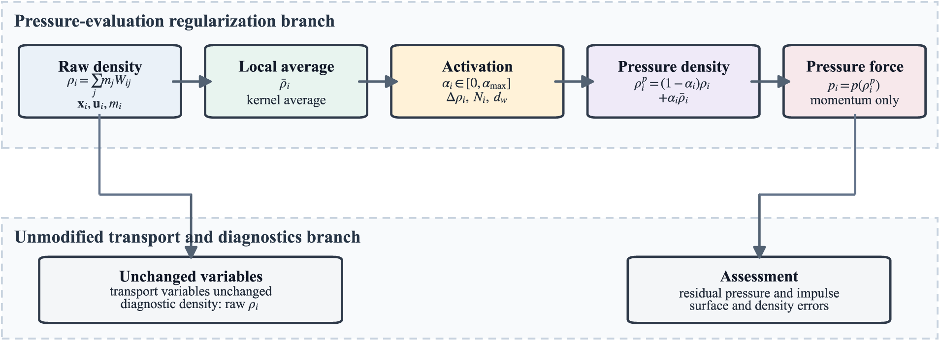
Figure 1: Schematic of the adaptive density regularization method, separating pressure evaluation from transport and diagnostics.

The simulations use the open source PySPH framework [44] as a reproducible SPH execution platform. PySPH is used as the implementation platform; the proposed contribution lies in the pressure evaluation sequence. Custom equation groups are inserted into the WCSPH solver sequence. The first group computes ρ¯i, the kernel sum normalization, and the neighbor count. The second group computes ηi, fiw, αi, and ρip. Pressure is then evaluated from ρip using the Tait equation of state. The subsequent momentum equation uses this pressure field, while all density denominators, particle volumes, acoustic speeds in artificial viscosity, and diagnostic density outputs remain evaluated from the raw summation density.

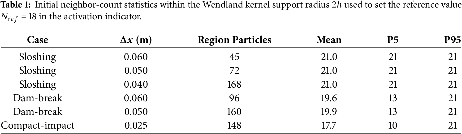
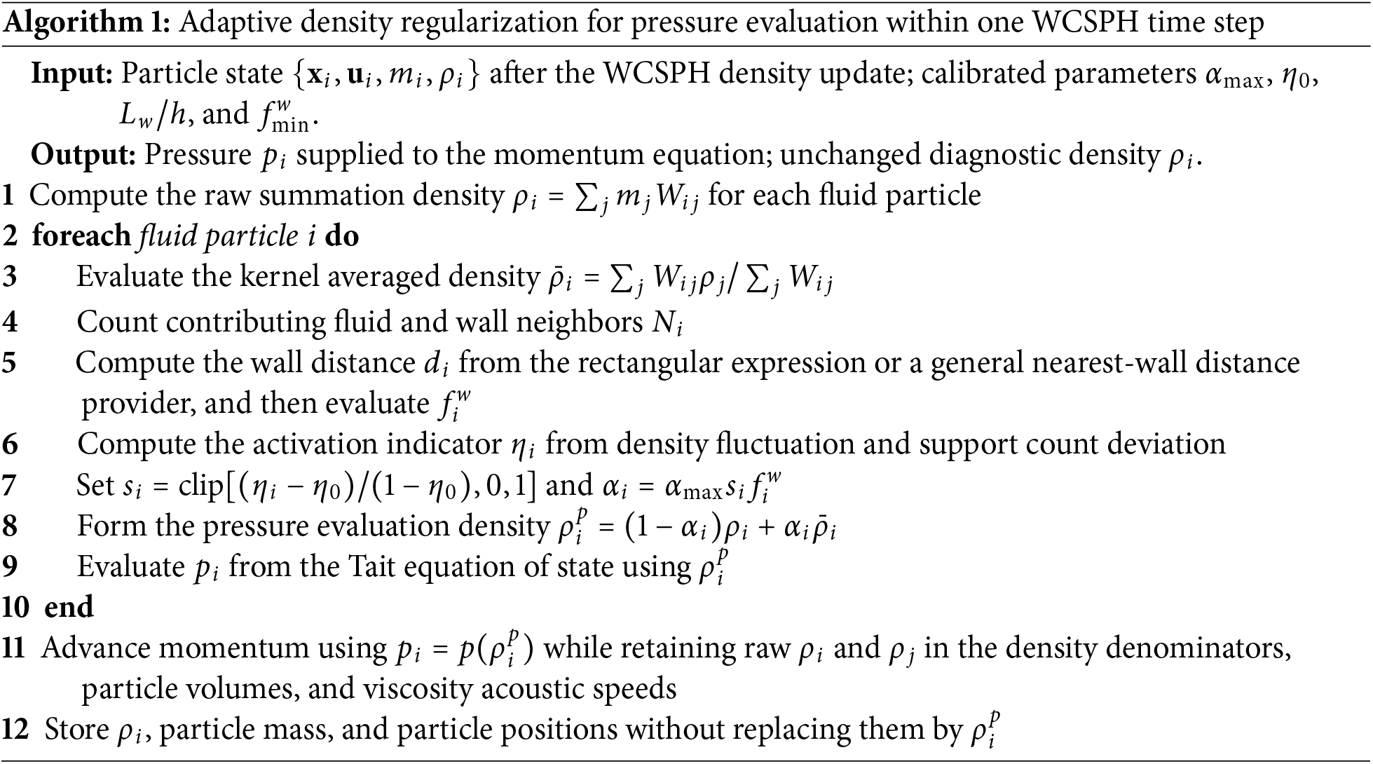
Algorithm 1 summarizes the pressure evaluation intervention. The pressure density blend exists only between the density update and the pressure evaluation. It is discarded after pressure is computed, so the output density field remains the raw summation density used by the baseline WCSPH formulation. The pairwise pressure-force operator therefore keeps the same density denominators and particle-volume definitions as the baseline solver; only the scalar pressure values entering this operator are changed. All four methods use the same particle layout, kernel, wall-particle discretization, artificial viscosity, and postprocessing definitions. The command line runner exposes the case, method, particle spacing, αmax, η0, wall proximity length, wall factor floor, wall model, and disorder-indicator weights, which makes the calibration and comparison sequence reproducible from scripts rather than reconstructed from manuscript descriptions.

4  Calibration and Computational Validation Design

4.1 Parameter Calibration

The parameter selection protocol uses a two dimensional dam break calibration case. The tank length is 2.0 m, the height is 1.2 m, and the initial water column is 0.58 m wide and 1.0 m high. The calibration particle spacing is Δx=0.06 m. The scan evaluates αmax=0.03, 0.05, and 0.10; η0=0.006 and 0.012; and Lw/h=1.5 and 2.0. The selection score combines normalized high frequency pressure energy, pressure standard deviation after impact, front position error, peak pressure change, positive pressure impulse change, an activation amplitude guard on α95,max, and a weak preference for shorter wall proximity support. Table 2 reports the selected parameters, which remain fixed in all subsequent numerical cases.

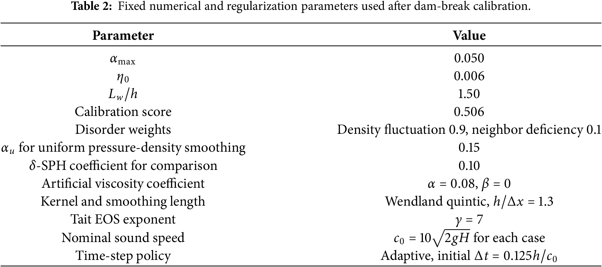
For each candidate parameter set θ=(αmax,η0,Lw/h), the calibration objective is

J(θ)=0.30E^HF+0.25σ^p+0.20E^f+0.10Δp^max+0.05ΔI^p+25.0[max(α95,max−0.003,0)0.003]2+0.20max(Lw/h−1.5,0).(18)

Here E^HF, σ^p, and E^f are the high frequency pressure energy, pressure standard deviation after impact, and front position error normalized by the baseline WCSPH calibration values. The terms Δp^max and ΔI^p are the absolute candidate to baseline changes in peak pressure and positive pressure impulse, normalized by the corresponding baseline magnitudes. The last two terms penalize broad activation and long wall proximity support. This objective selects one fixed parameter set before the sloshing, dam break, and compact impact runs are evaluated, so later comparisons do not use case specific tuning.

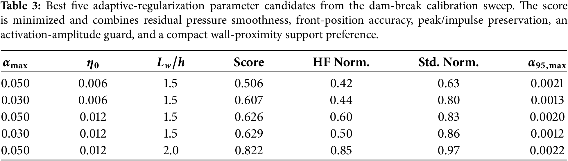
The calibration landscape is shown in Fig. 2, and Table 3 reports the five lowest score candidates. The selected setting is αmax=0.05, η0=0.006, and Lw/h=1.5. The next ranked candidates use the same compact wall support but different activation strength or threshold. Larger activation amplitudes and longer wall proximity support are penalized when they increase α95,max or broaden the correction. The selected set reduces pressure residuals while keeping the pressure density blend small and localized. The parameters are not tuned separately for the sloshing, dam break, or compact impact results. Their influence is assessed through the calibration landscape, the particle-spacing study, the wall-factor ablation, the indicator-weight sensitivity test, and the δ-SPH coefficient check reported in the Section 5.

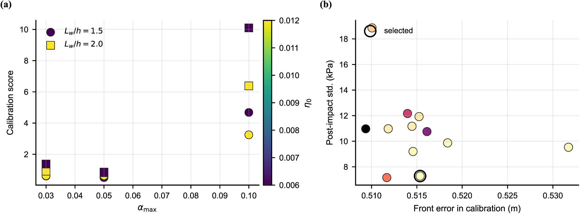
Figure 2: Dam break calibration landscape used to select the fixed adaptive regularization parameters: (a) calibration score as a function of αmax, with marker shape denoting Lw/h and color denoting η0; (b) post-impact pressure standard deviation vs. front-position error, with color denoting the calibration score and the selected setting circled.

4.2 Primary Sloshing Validation Case

The main comparison uses impulse induced sloshing in a rectangular tank of length 1.2 m and height 0.8 m. The initial water depth is 0.44 m. A horizontal velocity impulse is prescribed to the water column, with a weak vertical modulation to avoid rigid translation. Pressure probes are placed near the lower left and right side walls at y=0.12 m. The primary comparison uses Δx=0.05 m, final time 0.72 s, and the fixed calibrated parameters. Pressure RMSE, peak pressure error, pressure impulse error, and free surface height difference error are evaluated against a refined baseline SPH reference at Δx=0.04 m. A first mode sloshing reference is also plotted as a physical scale check for the pressure histories.

The impact window metrics are evaluated over the initial wall impact interval. The reported quantities are pressure time history RMSE, peak pressure error, pressure impulse error, high frequency pressure energy, pressure standard deviation after impact, free surface error, density fluctuation, mass conservation, and computational overhead. Pressure is also plotted in dimensionless form as p/(ρ0gH) and time as t(g/L)1/2.

4.3 Dam Break Case

A dam break case is retained as a second numerical case because it combines rapid front propagation, dry bed impact, and wall pressure oscillation, which are commonly used to assess free surface impact solvers [38]. The case uses the same tank and water column dimensions as the calibration stage, but changes the particle spacing to Δx=0.05 m. All regularization parameters remain fixed. The front position is compared with a shallow water front estimate, which is used as a kinematic scale reference rather than as a complete pressure benchmark. The metrics include front position RMSE, the delay for the front to reach xf=0.8L, right wall peak pressure, positive pressure impulse, high frequency pressure energy, density fluctuation, and pressure field snapshots.

4.4 Compact Water Mass Impact Case

The compact water mass impact case places a circular water patch of radius 0.18 m above the bottom wall of the same rectangular tank used for sloshing. The initial center is (0.60,0.42) m, and the water patch is assigned a downward velocity of 1.20 ms−1. The case is not intended as a surface-tension-resolved droplet benchmark. It provides a localized impact morphology for examining whether the pressure evaluation regularization changes the falling, impact, and spreading stages of a compact liquid mass. The bottom probes are located at (0.50,0.04) and (0.60,0.04) m, and the particle spacing is Δx=0.025 m.

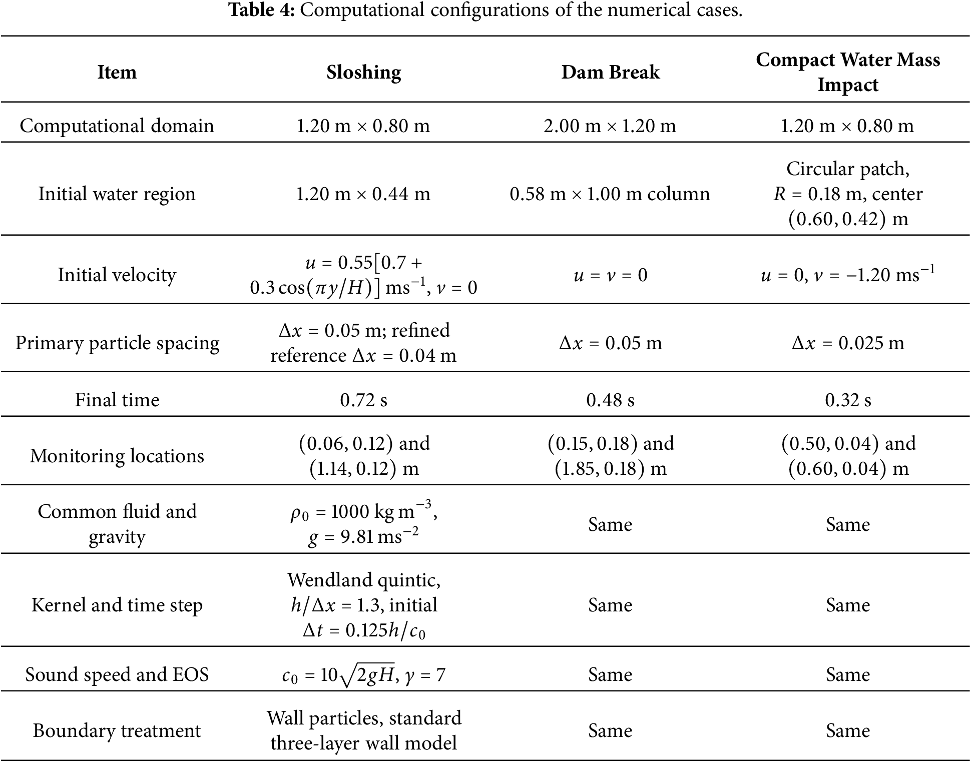
The computational configurations of the numerical cases are summarized in Table 4. All cases use the same fluid density, gravitational acceleration, Wendland kernel, smoothing length ratio, time-step policy, Tait equation exponent, wall-particle boundary treatment, and artificial-viscosity coefficient unless otherwise stated.

4.5 Evaluation Metrics

Pressure error is evaluated over the impact window [t1,t2] by comparing the simulated pressure trace p(t) with a reference trace pref(t). The pressure RMSE is defined as

ERMSE=[1Nt∑k=1Nt(p(tk)−pref(tk))2]1/2.(19)

The signed pressure impulse error is defined from the positive pressure impulse as

EI=∫t1t2max[p(t),0]dt−∫t1t2max[pref(t),0]dt∫t1t2max[pref(t),0]dt×100%.(20)

High frequency pressure energy is computed over the sloshing impact window t∈[0.15,0.55] s. For a pressure sequence pk=p(tk), a centered moving average trend with M samples is

p~k(M)=1|ℐk|∑ℓ∈ℐkpℓ,(21)

where ℐk is the available centered index set near k. The residual pressure is pk′=pk−p~k(M), and the high frequency pressure energy is

EHF(M)=1Nt∑k=1Nt(pk′)2.(22)

The reported main value uses M=7 and has units of kPa2. A separate window sensitivity check reports M=5, 7, and 11. For the spectral plot, pk′ is interpolated to a uniform time grid using the median sampling interval before computing a one sided normalized Fourier spectrum. Free surface error is measured from the tank height difference response, and density fluctuation is measured by the RMS value of (ρi−ρ0)/ρ0 over the fluid particles. These metrics are used together because pressure smoothing can improve one pressure statistic while worsening impulse conservation or free surface response.

5  Results and Model Assessment

5.1 Pressure Response in the Sloshing Validation Case

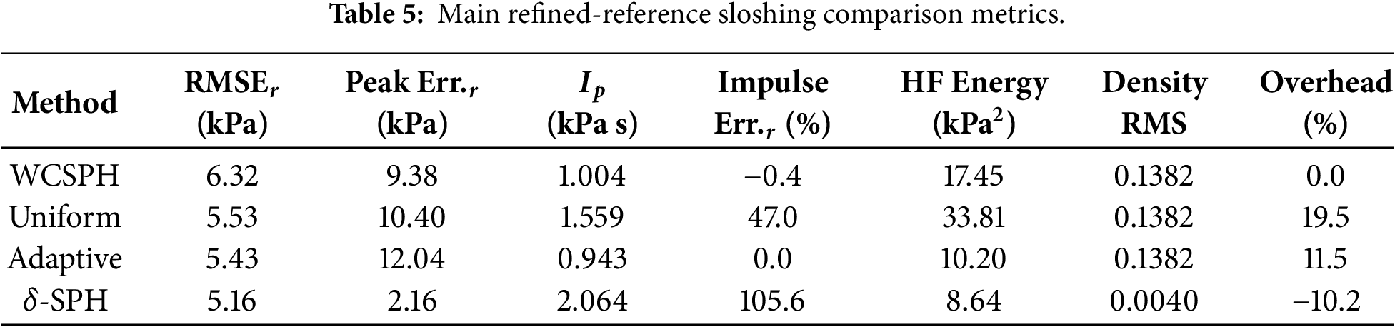
The main refined reference sloshing comparison is reported in Fig. 3 and Table 5. Against the refined SPH reference, the adaptive method reduces pressure RMSE from 6.32 to 5.43 kPa. Its main benefit appears in the high frequency part of the impact pressure signal, where the impact window energy falls from 17.45 to 10.20 kPa2, a 41.5% reduction. Uniform pressure density smoothing also lowers RMSE, but it increases residual pressure energy and produces a larger pressure impulse distortion. The tested δ-SPH configuration gives stronger high frequency damping in this sloshing case, while its signed pressure impulse error reaches 105.6%. This combination indicates that the δ-SPH trace is not dominated by an isolated pressure spike; rather, the smoothed pressure response changes the positive-pressure accumulation over the impact window. The adaptive correction therefore provides pressure smoothing with a smaller disturbance to impulse than the stronger density evolution stabilization baseline.

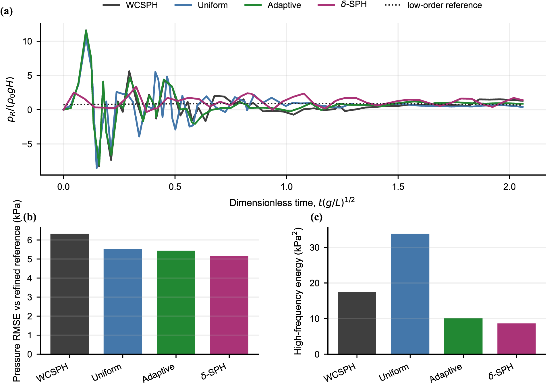
Figure 3: Main sloshing comparison among SPH stabilization methods: (a) dimensionless right-wall pressure histories; (b) pressure RMSE relative to the refined SPH reference; (c) high-frequency pressure energy. The first-mode sloshing reference in (a) is included only as a physical scale check.

The cumulative positive pressure impulse in Fig. 4 further separates pressure smoothing from load retention. The tested δ-SPH trace accumulates positive pressure more rapidly over the impact window, although its high frequency residual is smaller than that of the other methods. The adaptive curve remains closer to the refined reference accumulation while still lowering the high frequency residual pressure energy. This result supports the interpretation that the large relative impulse error of the tested δ-SPH case is a window-integrated response difference under the present coefficient and boundary setup, not a single unstable pressure excursion.

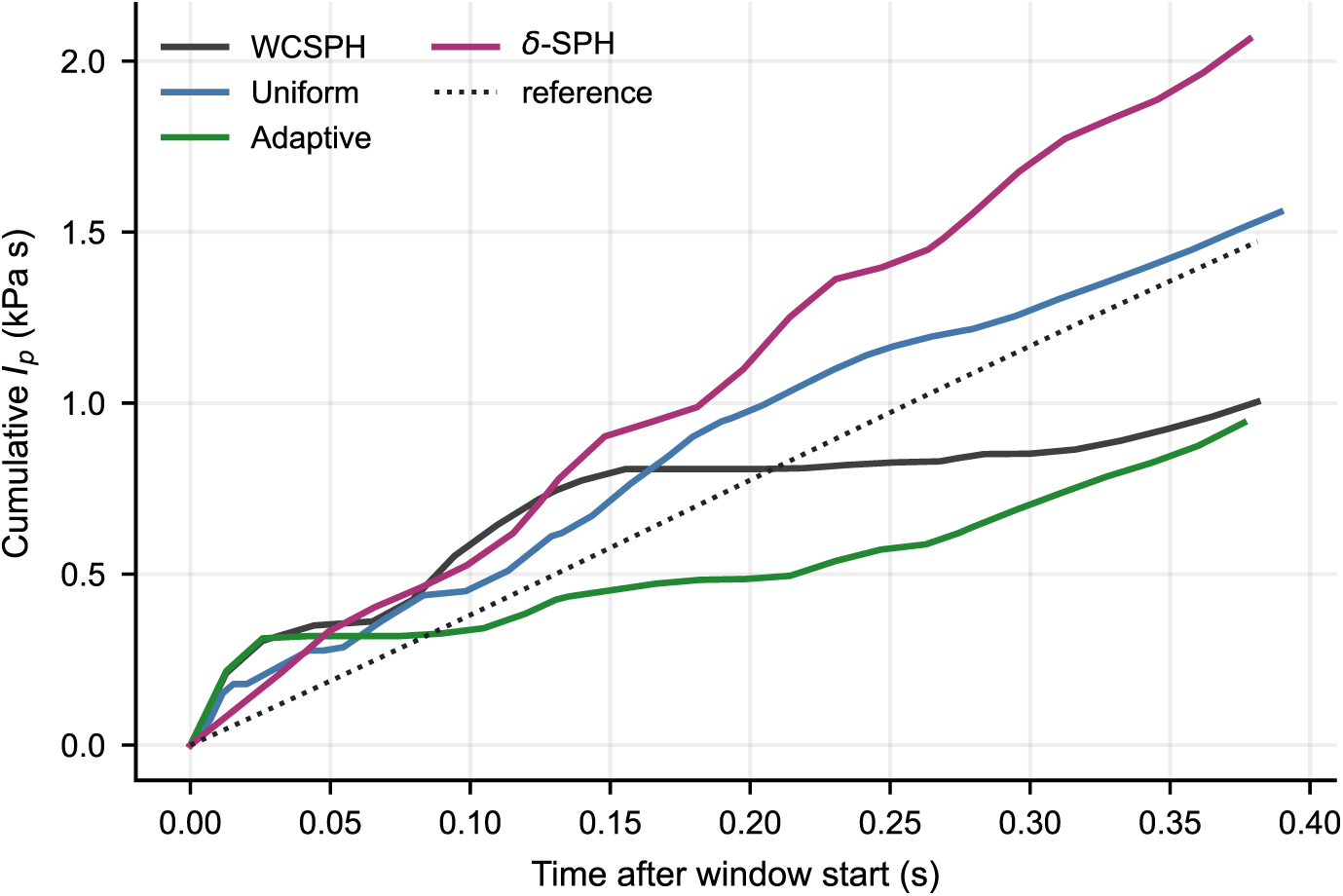
Figure 4: Cumulative positive pressure impulse in the sloshing impact window, showing the load accumulation associated with each stabilization method.

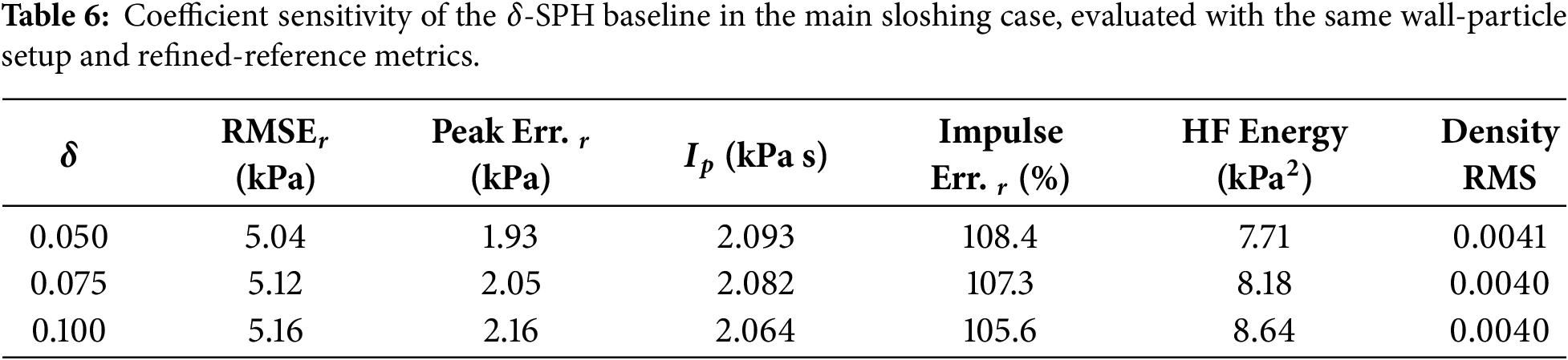
Table 6 reports a coefficient sensitivity check for the δ-SPH baseline. The purpose is not to retune the competing method for each figure, but to show how the pressure damping and impulse accumulation vary when the density diffusion coefficient is changed under the same particle spacing, wall treatment, and postprocessing window. The comparison keeps the proposed adaptive parameters fixed and uses the same refined reference metrics as the main sloshing table.

The pressure and response metrics normalized by baseline WCSPH are summarized in Fig. 5. Adaptive regularization improves refined reference pressure RMSE, high frequency energy, and smoothness after impact while keeping free surface error close to the baseline value. It does not minimize peak pressure error, as expected for a local regularization that is not fitted to peak load. Pressure impulse error is plotted separately because the baseline impulse error is close to zero and is not a stable normalization denominator. The added density averaging and activation equations increase runtime, but the overhead remains moderate in the present cases.

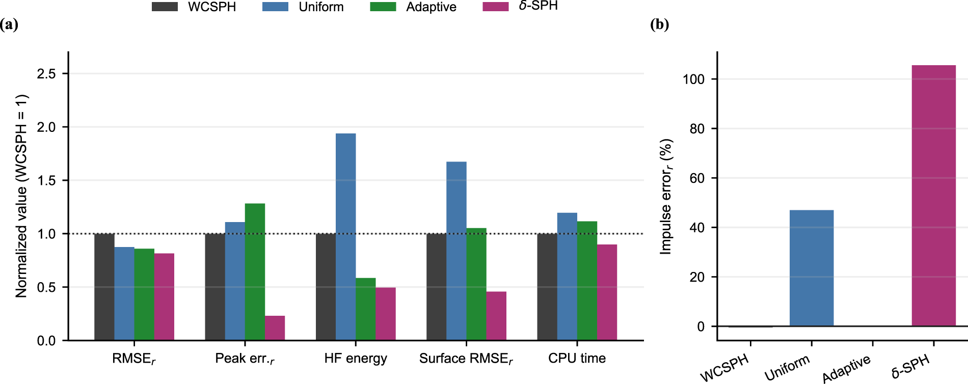
Figure 5: Normalized sloshing response metrics: (a) pressure RMSE, peak-pressure error, high-frequency energy, free-surface RMSE, and runtime normalized by the WCSPH values; (b) signed positive-pressure impulse error relative to the refined SPH reference.

The pressure smoothing and response retention balance is summarized in Fig. 6. In the sloshing case, adaptive regularization reduces high frequency pressure energy to 0.58 times the WCSPH value and keeps the refined reference impulse error at 0.0%. The tested δ-SPH configuration reduces high frequency energy further, but the impulse error increases to 105.6%. In the compact impact case, the adaptive method preserves the WCSPH peak pressure almost unchanged, whereas δ-SPH reduces it by 56.5%. These results show a moderate pressure regularization effect with stronger retention of peak and impulse measures in the present benchmark set.

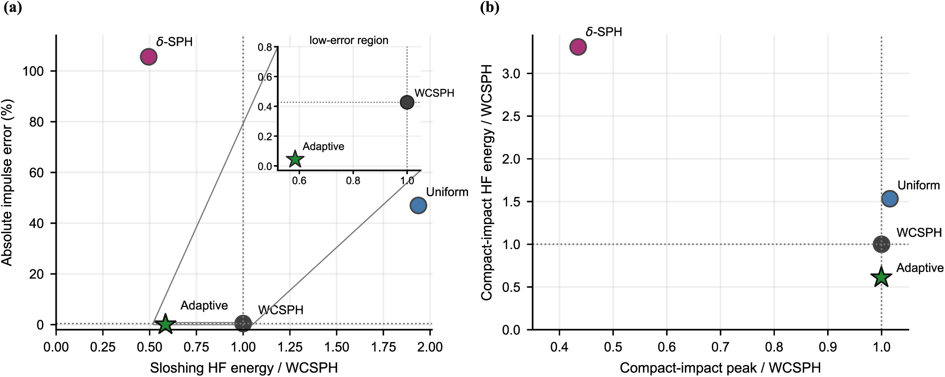
Figure 6: Balance between pressure smoothing and response retention: (a) normalized sloshing high-frequency energy vs. absolute impulse error, with an inset magnifying the low-error region; (b) normalized compact-impact peak pressure vs. high-frequency energy.

The same metrics are summarized in the diagnostic matrix in Fig. 7 as signed changes relative to WCSPH. Negative high frequency energy changes denote pressure damping, whereas values close to zero in the impulse, compact peak, and density RMS columns indicate response retention. Uniform smoothing increases high frequency energy and impulse error in this comparison. Adaptive regularization reduces high frequency energy while keeping the impulse error, compact impact peak, and density RMS close to WCSPH. The δ-SPH result gives stronger high frequency damping, but it also produces larger impulse, compact peak, and density RMS changes under the tested coefficient and wall-particle setup.

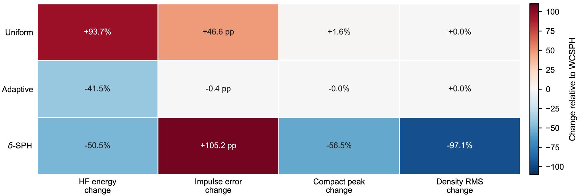
Figure 7: Signed diagnostic changes relative to WCSPH for pressure damping and response retention metrics.

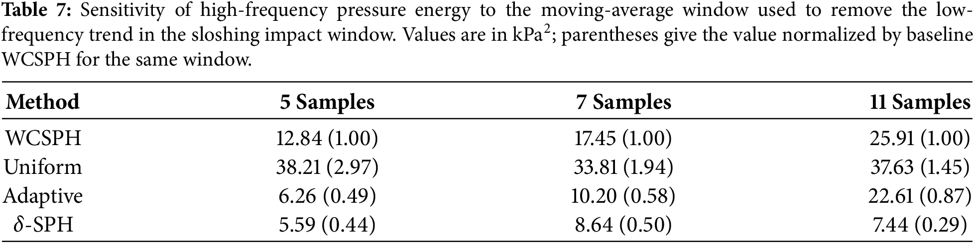
Residual pressure spectra and window sensitivity are shown in Fig. 8 and Table 7. The spectrum is computed after subtracting a centered moving average trend from the impact window pressure. Adaptive regularization gives lower residual energy than WCSPH for all three windows. The reduction weakens for the longest window because a longer moving average filter assigns more intermediate frequency content to the residual. The tested δ-SPH configuration gives an even lower residual pressure energy in this sloshing signal, whereas uniform smoothing does not. The exact reduction percentage depends on the filter window, but the direction of the adaptive effect is stable.

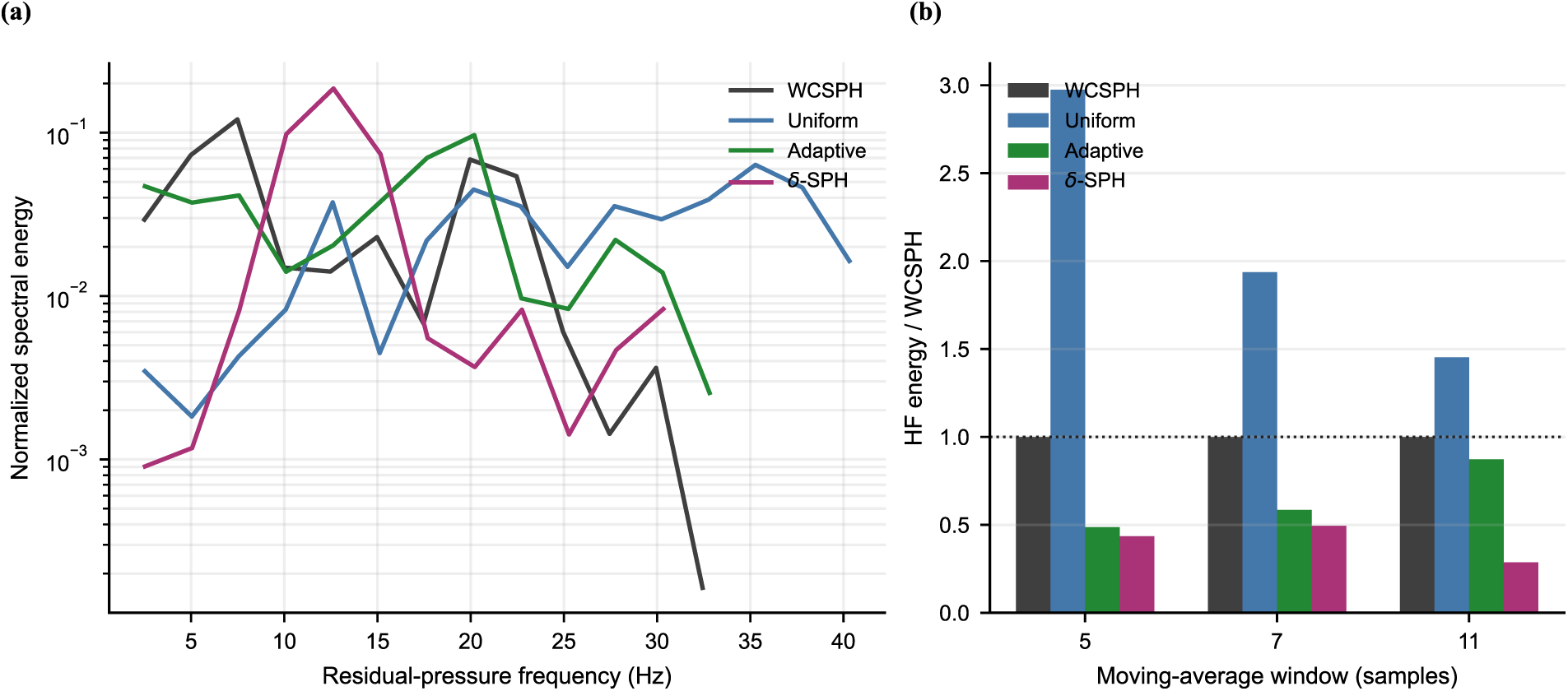
Figure 8: Sloshing impact signal diagnostics: (a) normalized residual-pressure spectra; (b) high-frequency pressure energy for moving-average windows of 5, 7, and 11 samples.

Particle level pressure fields and the corresponding flow morphology are compared in Fig. 9. All rows use the same particle spacing, time instants, and pressure color scale. Adaptive regularization preserves the global sloshing shape seen in WCSPH while reducing localized high pressure speckle relative to the more uniformly smoothed alternatives. The particle field comparison shows that the pressure improvement is not obtained by visibly changing the bulk free surface evolution.

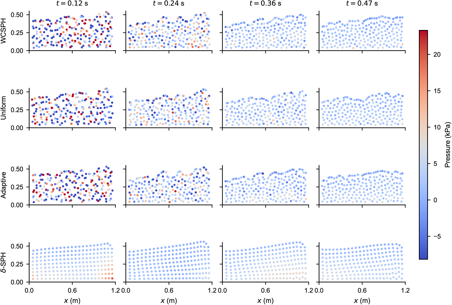
Figure 9: Particle-level pressure fields for the main sloshing case. Columns show the selected impact times, and rows show WCSPH, uniform smoothing, adaptive regularization, and δ-SPH.

Grid reconstructed pressure contours from the same particle data are shown in Fig. 10. Particle pressure is interpolated onto a fixed Cartesian grid, and grid points outside the particle supported fluid region are masked. The contours are used only for visualization; all quantitative metrics are computed from the original SPH probe and particle data. In this view, adaptive regularization reduces scattered high pressure patches while retaining a free surface envelope close to the baseline WCSPH solution.

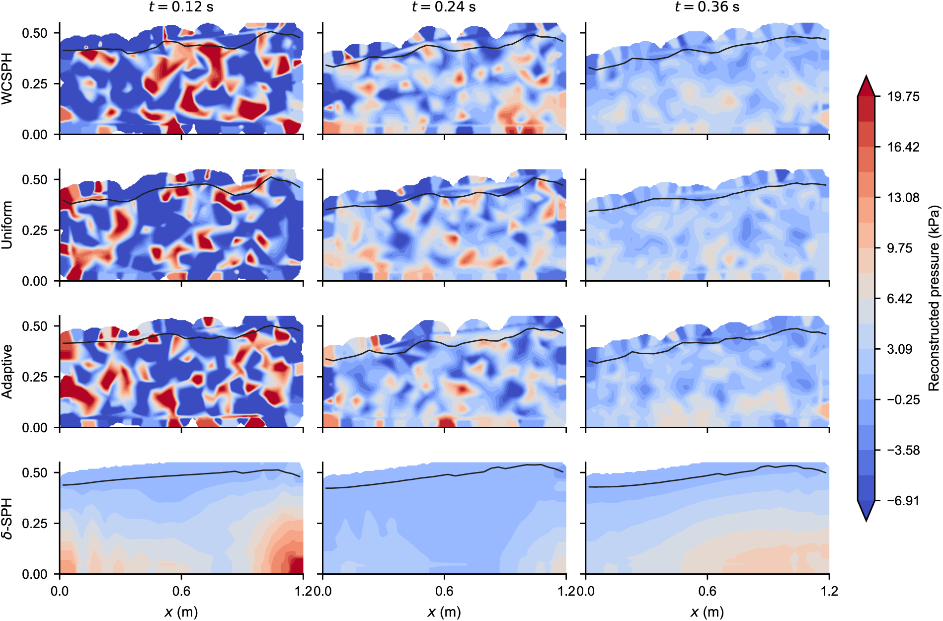
Figure 10: Grid-reconstructed pressure contours from SPH particle data in the main sloshing case. Columns show the selected impact times, and rows show WCSPH, uniform smoothing, adaptive regularization, and δ-SPH.

Extracted free surface envelopes are shown in Fig. 11. During the wall impact interval, the adaptive curve follows the WCSPH free surface morphology closely. Uniform smoothing and δ-SPH show different stabilization balances. The close agreement between the adaptive and WCSPH envelopes shows that the main change occurs in pressure evaluation rather than liquid surface motion.

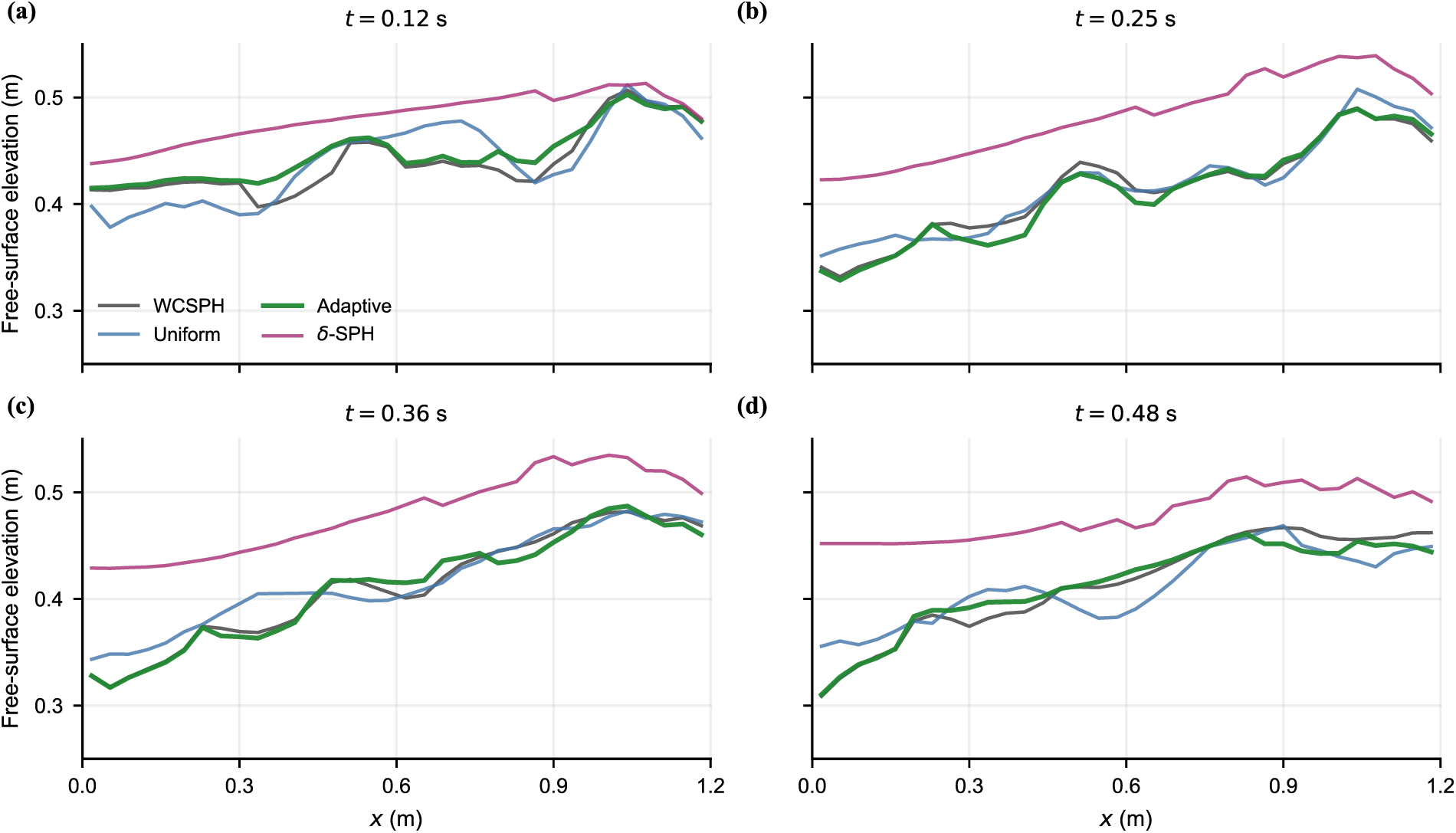
Figure 11: Extracted free-surface envelopes for WCSPH, uniform smoothing, adaptive regularization, and δ-SPH at (a) t=0.12 s, (b) t=0.25 s, (c) t=0.36 s, and (d) t=0.48 s.

The refined reference free surface error remains close to the baseline value, and mass is conserved to the reported precision because particle masses are unchanged. Mean density RMS also remains at the baseline level because the adaptive method does not replace diagnostic density. This separates the proposed module from δ-SPH. The latter gives stronger density stabilization by modifying density evolution, whereas the proposed module separates diagnostic density from pressure regularization. The computational overhead is 11.5% for this small case, mainly from the additional local density and activation equation groups.

5.2 Resolution, Wall Activation, and Secondary Cases

Resolution and wall activation sensitivity are shown in Table 8 and Fig. 12. The sloshing case is repeated at Δx=0.06, 0.05, and 0.04 m. At Δx=0.04 m, adaptive regularization reduces pressure RMSE from 3.56 to 3.24 kPa. At Δx=0.05 m and Δx=0.06 m, RMSE remains close to the baseline value, while high frequency pressure energy is reduced at all three spacings. Across the three spacings, the adaptive method reduces pressure fluctuation after impact or high frequency energy without changing particle mass or diagnostic density.

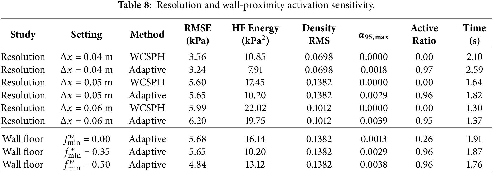
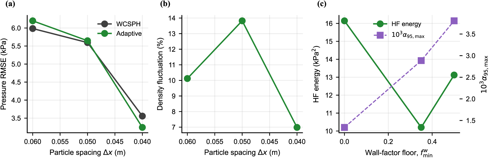
Figure 12: Particle spacing and wall activation sensitivity: (a) pressure RMSE vs. particle spacing; (b) density fluctuation vs. particle spacing; (c) high-frequency pressure energy and the 95th-percentile maximum activation vs. the wall-factor floor.

The particle spacing panel is restricted to WCSPH and the proposed pressure evaluation regularization method because the δ-SPH rows require separate interpretation. In diagnostic runs, the coarse Δx=0.06 m δ-SPH pressure trace gives an unusually small RMSE against the first-mode sloshing reference introduced in Section 4.2 as a physical scale check, but the same trace has a strongly damped pressure peak. This reflects filter and reference alignment, not monotone pressure convergence. The tested δ-SPH configuration is retained in the method comparison, dam break, and compact impact sections. The resolution panel instead assesses the proposed module relative to its underlying WCSPH route.

The wall proximity ablation varies the lower bound fminw while keeping αmax, η0, and Lw/h fixed. Setting fminw=0 confines activation mostly to particles near the wall and reduces the mean active ratio to 0.26, but high frequency pressure energy remains 16.14 kPa2. The calibrated value, fminw=0.35, gives the lowest high frequency energy, 10.20 kPa2, with α95,max=0.0029. Increasing the floor to 0.50 improves RMSE and impulse error in this case, but high frequency energy rises to 13.12 kPa2. The ablation shows that the wall proximity factor changes both the activation pattern and the pressure metrics. It is not a passive geometric multiplier.

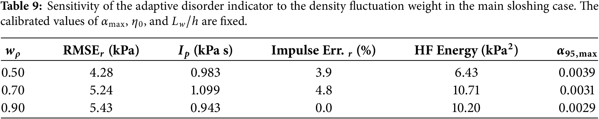
Table 9 examines the density fluctuation weight in the disorder indicator while keeping the calibrated regularization parameters fixed. Increasing wρ emphasizes the equation of state sensitive density fluctuation, whereas decreasing it gives more weight to support count deficiency. The selected value wρ=0.9 follows this density dominated interpretation and keeps the support count term as a secondary localization cue rather than a second tuning route.

Pressure and activation maps in Fig. 13 illustrate the regularization mechanism. The adaptive coefficient remains small because it is bounded by the calibrated αmax and by the local activation indicator. Nonzero regions appear near the disturbed free surface and wall impact zone, where density fluctuation, support count deviation, and wall proximity information combine. The pressure maps show local damping of pressure speckle without replacement of the bulk sloshing pattern. The active regions coincide with locations where the pressure field is most irregular, while the large scale free surface response remains close to WCSPH.

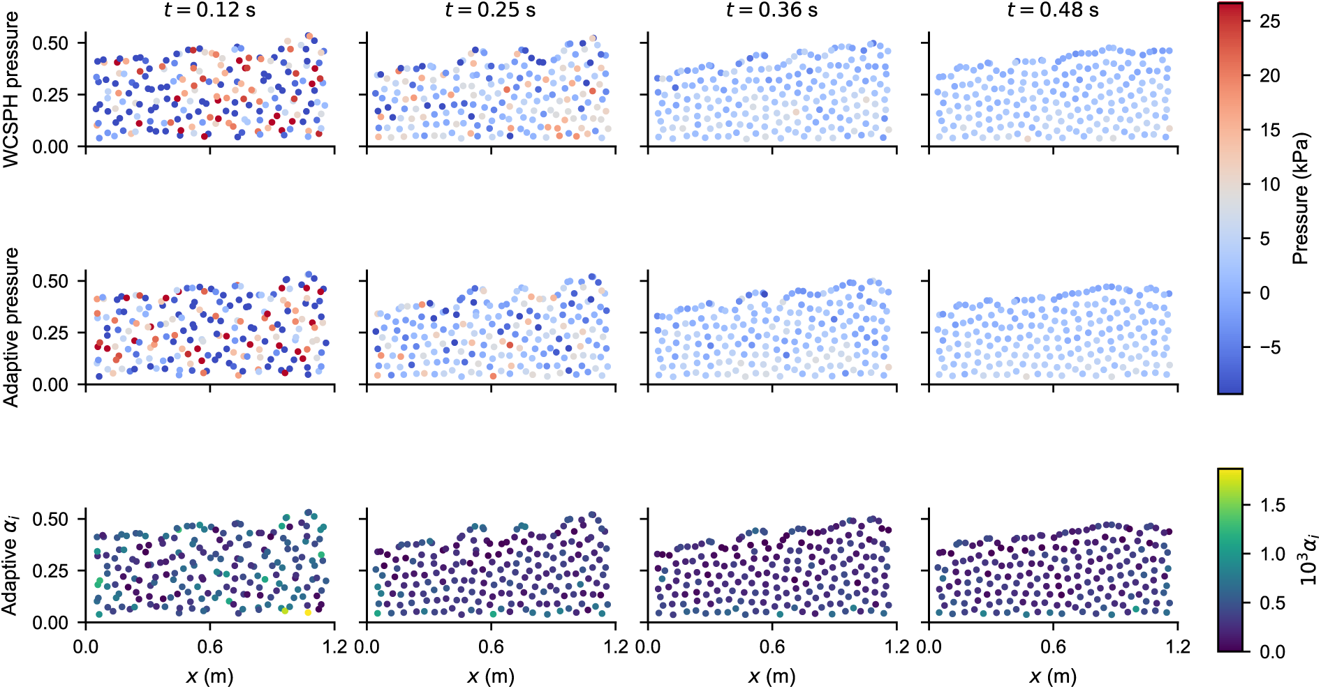
Figure 13: Sloshing pressure fields and adaptive activation maps during the wall-impact interval. Columns show the selected times; rows show WCSPH pressure, adaptive pressure, and the adaptive activation coefficient αi.

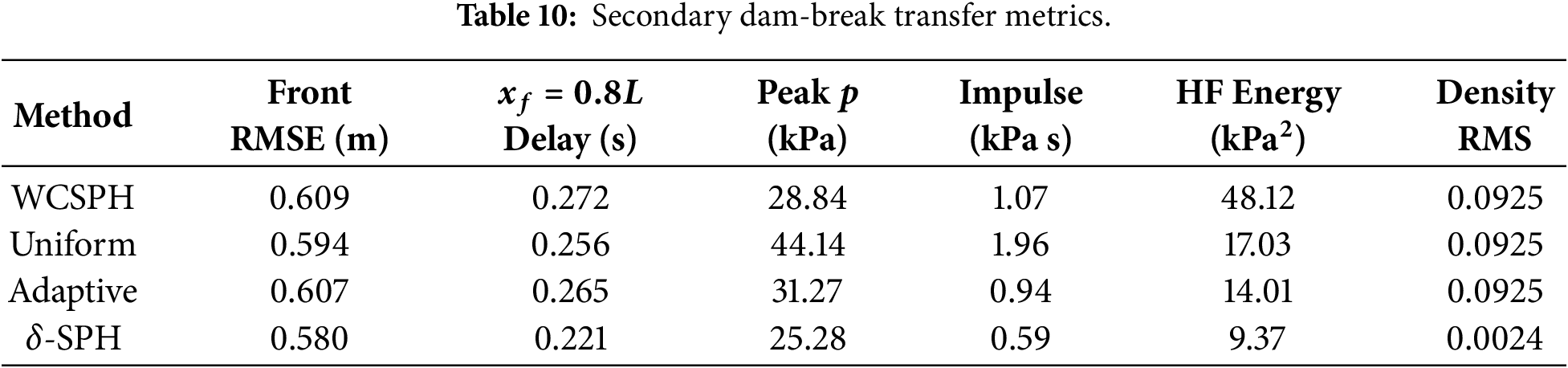
The fixed parameter result in a second free surface impact geometry is shown in Fig. 14 and Table 10. All four methods propagate the front more slowly than the shallow water estimate, as expected for the present resolved particle calculation with wall support and pressure stabilization terms. Adaptive regularization stays close to baseline WCSPH in front RMSE, arrival delay, and peak pressure, while reducing high frequency pressure energy from 48.12 to 14.01 kPa2. The tested δ-SPH configuration gives the strongest density stabilization and the lowest high frequency pressure energy in this case, but it also changes pressure impulse relative to WCSPH. The dam break results follow the same pattern as the sloshing results: adaptive regularization reduces high frequency pressure content while keeping front motion and peak pressure close to WCSPH.

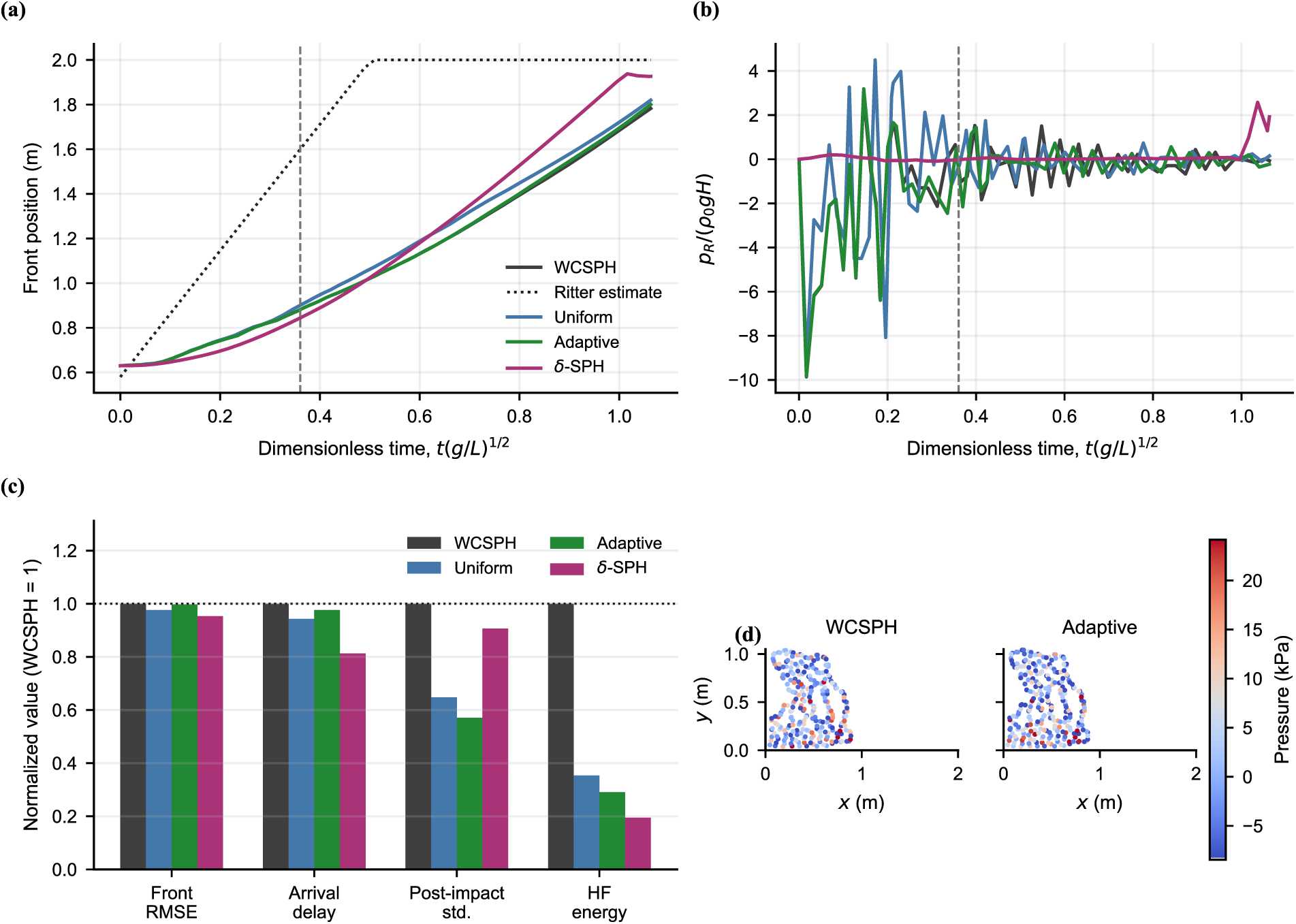
Figure 14: Dam break check: (a) front-position histories; (b) right-wall pressure histories; (c) normalized response metrics; (d) WCSPH and adaptive particle-pressure fields at the selected time.

5.3 Compact Water Mass Impact Case

The compact impact case in Fig. 15 and Table 11 gives a more localized morphology. A two dimensional circular water patch is assigned an initial downward velocity and impacts the bottom wall. Surface tension and contact angle physics are not included, so the case is not a surface tension resolved droplet benchmark. The case examines whether the pressure evaluation regularization behavior observed in sloshing and dam break flow is also obtained in a compact impact geometry.

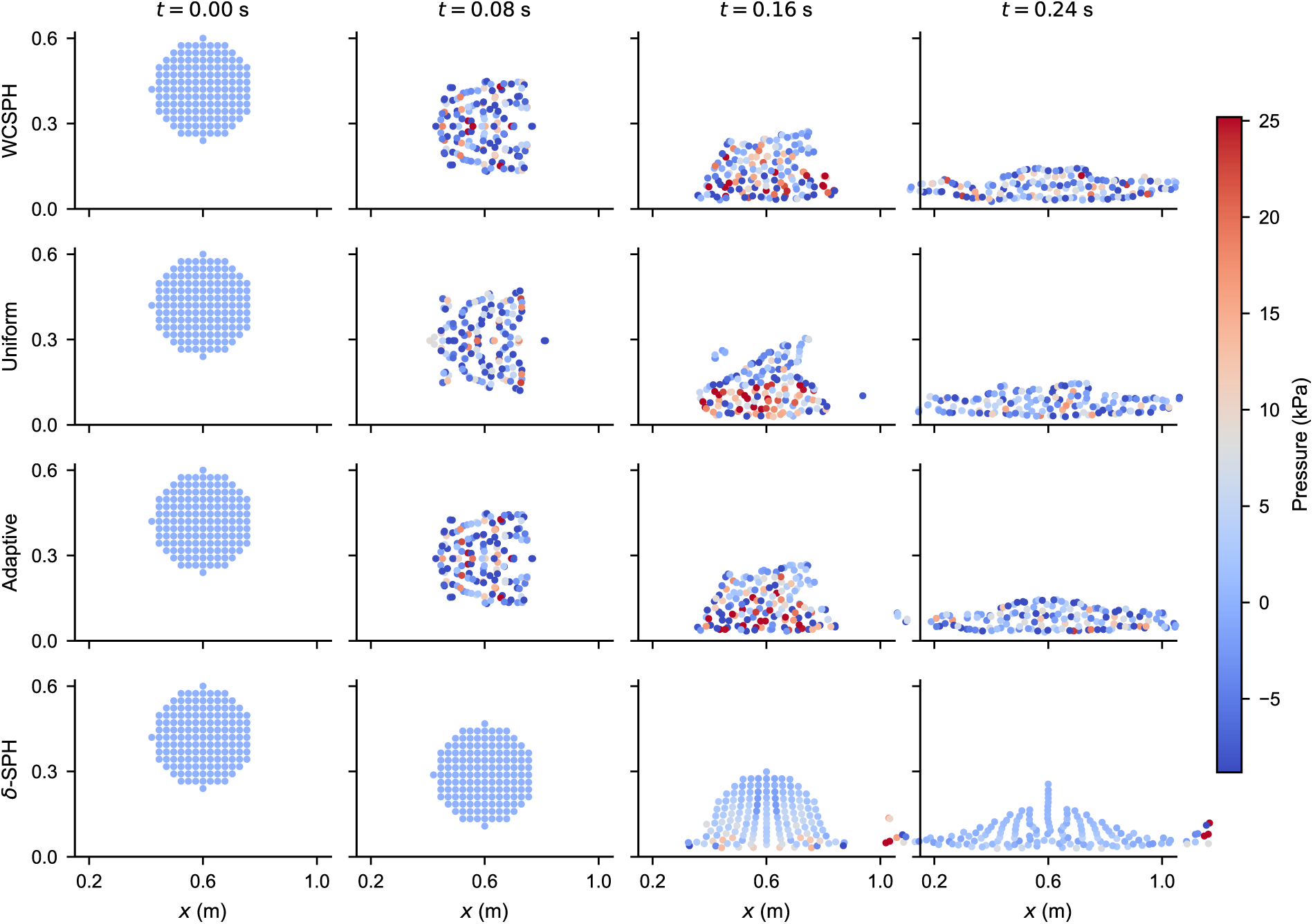
Figure 15: Compact water mass impact particle-pressure fields during falling, impact, and spreading. Columns show the selected times, and rows show WCSPH, uniform smoothing, adaptive regularization, and δ-SPH.

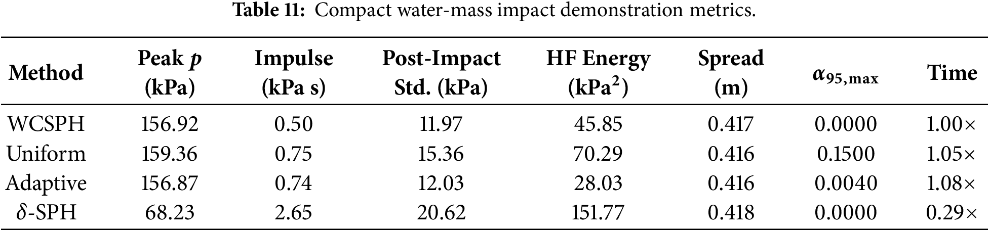
The adaptive method retains the falling, impact, and spreading stages observed in baseline WCSPH. The pressure field changes locally, while the global morphology remains close to the baseline solution. Compact impact metrics show the same balance seen in the sloshing case. Adaptive regularization keeps peak pressure close to WCSPH, whereas δ-SPH strongly lowers the peak pressure and increases the high frequency residual for this morphology. The corresponding bottom probe histories and activation maps are shown in Fig. 16. The pressure peak, residual energy, and activation maps show a local pressure correction rather than a prescribed change in bulk motion.

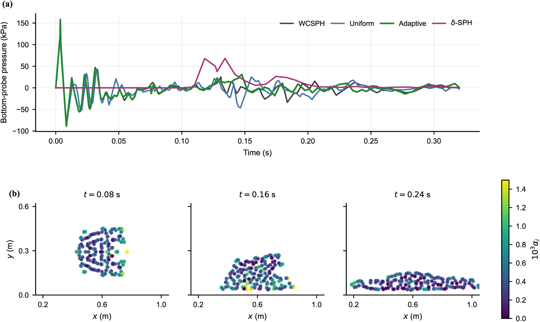
Figure 16: Compact impact response: (a) pressure histories at the two bottom probes; (b) adaptive activation maps at the selected impact times.

5.4 Scope and Balances

Across the numerical cases, the compared methods show distinct balances among pressure damping, impulse preservation, compact impact peak response, and diagnostic density retention. Adaptive regularization does not minimize every metric. Uniform smoothing attains a competitive RMSE against the refined sloshing reference, but it increases high frequency pressure energy and shifts the positive pressure impulse. The tested δ-SPH configuration gives stronger density stabilization and lower high frequency energy in the main sloshing case, whereas its refined reference impulse error is larger and its compact impact peak response departs more strongly from WCSPH. These results indicate that high frequency energy alone is insufficient for judging impact pressure stabilization. A joint assessment of damping benefit, impulse preservation, compact impact peak retention, and diagnostic density behavior characterizes the proposed module as a response preserving pressure regularization rather than a maximum damping filter.

This balance follows from the pressure evaluation design. Because ρip is introduced only in the equation of state, the method regularizes the pressure field supplied to the momentum equation without overwriting the raw density used for diagnostics, particle volume, or pressure gradient denominators. Such separation is advantageous when pressure traces contain nonphysical oscillations while free surface motion and density diagnostics remain acceptable. Activation maps further show that the correction is guided by density fluctuation, support count deviation, and wall proximity indicators instead of being imposed as a domain wide filter. Although αi remains small, the Tait equation of state amplifies density perturbations into pressure fluctuations; a limited pressure density blend can therefore reduce high frequency content without substantially changing diagnostic density statistics.

Practical use still requires attention to validation scope and geometry. The main pressure error metrics in this study are referenced to a refined SPH solution rather than a dedicated experimental pressure trace, and the first-mode sloshing reference is used only as a physical scale check. The δ-SPH comparison uses one representative coefficient in the main table, so coefficient specific impulse behavior should not be interpreted as a general limitation of δ-SPH. The coordinate aligned wall distance used for the rectangular tanks does not directly cover curved walls, internal baffles, multiply connected domains, or moving boundaries. For such geometries, the wall factor should be driven by a signed distance field, a closest surface query, or a boundary particle projection, with the wall length scale and support reference reassessed for the local support pattern. Future work should extend the same pressure regularization idea to experimental impact pressure datasets, three dimensional sloshing, hydroelastic response, multiphase flows, particle shifting schemes, and more general wall boundary formulations.

6  Conclusions

This work developed an adaptive density regularization method for pressure evaluation in WCSPH modeling of free surface impact flows. The method constructs a local kernel averaged density and blends it with the raw summation density only for pressure evaluation through the Tait equation of state, while particle mass, particle volume, pressure-gradient density denominators, and diagnostic density retain their baseline WCSPH definitions. The fixed parameter comparison shows that the proposed method reduces high frequency pressure oscillations in the sloshing validation case while keeping the free surface morphology, pressure impulse, and diagnostic density close to the baseline WCSPH solution. The dam break and compact water mass impact cases give the same qualitative response. Compared with uniform smoothing, the adaptive coefficient avoids domain wide pressure density filtering; compared with the tested δ-SPH configuration, it gives a milder correction that better preserves response related quantities in the tested configurations. Further work should extend the assessment to three dimensional impact cases, experimental pressure datasets, advanced wall models, particle shifting, hydroelastic response, multiphase effects, and general wall-distance providers for curved or baffled geometries.

Acknowledgement: Not applicable.

Funding Statement: This work was supported by the Shandong Provincial Natural Science Foundation, grant number ZR2025QC44; the Ph.D. Research Startup Foundation of Shandong University of Aeronautics, grant number 2025Y24; and the project titled Research on the General Aviation Industry Development Plan of Shandong Province, grant number BZXYQNLG202005.

Author Contributions: The authors confirm contribution to the paper as follows: conceptualization, Fan Cao and Maopeng Tian; methodology, Fan Cao and Xinlei He; software, Fan Cao; validation, Maopeng Tian and Fan Cao; formal analysis, Maopeng Tian, Fan Cao and Xinlei He; investigation, Maopeng Tian; resources, Fan Cao and Caicheng Zhu; data curation, Maopeng Tian and Fan Cao; writing—original draft preparation, Maopeng Tian and Fan Cao; writing—review and editing, Xinlei He, Fan Cao and Caicheng Zhu; visualization, Maopeng Tian; supervision, Fan Cao; project administration, Fan Cao; funding acquisition, Fan Cao. All authors reviewed and approved the final version of the manuscript.

Availability of Data and Materials: The data and scripts supporting the findings of this study are available from the corresponding author upon reasonable request.

Ethics Approval: Not applicable.

Conflicts of Interest: The authors declare no conflicts of interest.

References

1. Lyu HG, Sun PN, Huang XT, Zhong SY, Peng YX, Jiang T, et al. A review of SPH techniques for hydrodynamic simulations of ocean energy devices. Energies. 2022;15(2):502. doi:10.3390/en15020502. [Google Scholar] [CrossRef]

2. Bagheri M, Mohammadi M, Riazi M. A review of smoothed particle hydrodynamics. Comput Part Mech. 2024;11(3):1163–219. doi:10.1007/s40571-023-00679-7. [Google Scholar] [CrossRef]

3. Gingold RA, Monaghan JJ. Smoothed particle hydrodynamics: theory and application to non-spherical stars. Mon Not R Astron Soc. 1977;181(3):375–89. doi:10.1093/mnras/181.3.375. [Google Scholar] [CrossRef]

4. Monaghan JJ. Smoothed particle hydrodynamics. Annu Rev Astron Astrophys. 1992;30(1):543–74. doi:10.1146/annurev.aa.30.090192.002551. [Google Scholar] [CrossRef]

5. Monaghan JJ. Smoothed particle hydrodynamics. Rep Prog Phys. 2005;68(8):1703–59. doi:10.1088/0034-4885/68/8/R01. [Google Scholar] [CrossRef]

6. Monaghan JJ. Simulating free surface flows with SPH. J Comput Phys. 1994;110(2):399–406. doi:10.1006/jcph.1994.1034. [Google Scholar] [CrossRef]

7. Dalrymple RA, Rogers BD. Numerical modeling of water waves with the SPH method. Coast Eng. 2006;53(2–3):141–7. doi:10.1016/j.coastaleng.2005.10.004. [Google Scholar] [CrossRef]

8. Gómez-Gesteira M, Rogers BD, Dalrymple RA, Crespo AJC. State-of-the-art of classical SPH for free-surface flows. J Hydraul Res. 2010;48(sup1):6–27. doi:10.1080/00221686.2010.9641242. [Google Scholar] [CrossRef]

9. Zhang C, Zhu YJ, Wu D, Adams NA, Hu XY. Smoothed particle hydrodynamics: methodology development and recent achievement. J Hydrodyn. 2022;34(5):767–805. doi:10.1007/s42241-022-0052-1. [Google Scholar] [CrossRef]

10. Pozorski J, Olejnik M. Smoothed particle hydrodynamics modelling of multiphase flows: an overview. Acta Mech. 2023;235(4):1685–714. doi:10.1007/s00707-023-03763-4. [Google Scholar] [CrossRef]

11. Li H, Zhang X, Yang X. Numerical study of liquid sloshing using smoothed particle hydrodynamics with adaptive spatial resolution. Eng Anal Bound Elem. 2024;159(6):272–87. doi:10.1016/j.enganabound.2023.12.006. [Google Scholar] [CrossRef]

12. Liu WB, Ma DJ, Qian JZ, Zhang MY, He AM, Liu NS, et al. High-accuracy three-dimensional surface detection in smoothed particle hydrodynamics for free-surface flows. Comput Phys Commun. 2023;290(3):108789. doi:10.1016/j.cpc.2023.108789. [Google Scholar] [CrossRef]

13. Crespo AJC, Domínguez JM, Rogers BD, Gómez-Gesteira M, Longshaw S, Canelas R, et al. DualSPHysics: open-source parallel CFD solver based on smoothed particle hydrodynamics. Comput Phys Commun. 2015;187(6):204–16. doi:10.1016/j.cpc.2014.10.004. [Google Scholar] [CrossRef]

14. Domínguez JM, Crespo AJC, Gómez-Gesteira M. Optimization strategies for CPU and GPU implementations of a smoothed particle hydrodynamics method. Comput Phys Commun. 2013;184(3):617–27. doi:10.1016/j.cpc.2012.10.015. [Google Scholar] [CrossRef]

15. Barreiro A, Crespo AJC, Domínguez JM, Gómez-Gesteira M. Smoothed particle hydrodynamics for coastal engineering problems. Comput Struct. 2013;120(12):96–106. doi:10.1016/j.compstruc.2013.02.010. [Google Scholar] [CrossRef]

16. Zhang S, Zhang J, Li X, Wang J, Huang C. Mechanisms of seepage and overtopping-induced failure in earthen dams: a coupled two-layer SPH investigation. Comput Geotech. 2026;198:108344. doi:10.1016/j.compgeo.2026.108344. [Google Scholar] [CrossRef]

17. Xu X, Wang E, Li X, Yu P. An improved weakly compressible SPH method for simulating 2D multiphase flows with complex interface and large density ratios. Eng Anal Bound Elem. 2024;169:106043. doi:10.1016/j.enganabound.2024.106043. [Google Scholar] [CrossRef]

18. Wang XJ, Huang C, Yan WH, Aly AM, Zhao QL, He GP. Study on hydrodynamic characteristics of multiple fish based on smoothed particle hydrodynamics. Phys Fluids. 2024;36(11):111915. doi:10.1063/5.0236386. [Google Scholar] [CrossRef]

19. Koshizuka S, Oka Y. Moving-particle semi-implicit method for fragmentation of incompressible fluid. Nucl Sci Eng. 1996;123(3):421–34. doi:10.13182/NSE96-A24205. [Google Scholar] [CrossRef]

20. Shao S, Lo EYM. Incompressible SPH method for simulating Newtonian and non-Newtonian flows with a free surface. Adv Water Resour. 2003;26(7):787–800. doi:10.1016/S0309-1708(03)00030-7. [Google Scholar] [CrossRef]

21. Lee ES, Moulinec C, Xu R, Violeau D, Laurence D, Stansby P. Comparisons of weakly compressible and truly incompressible algorithms for the SPH mesh free particle method. J Comput Phys. 2008;227(18):8417–36. doi:10.1016/j.jcp.2008.06.005. [Google Scholar] [CrossRef]

22. Hu XY, Adams NA. An incompressible multi-phase SPH method. J Comput Phys. 2007;227(1):264–78. doi:10.1016/j.jcp.2007.07.013. [Google Scholar] [CrossRef]

23. Zhang N, Yan S, Ma Q, Guo X, Xie Z, Zheng X. A CNN-supported Lagrangian ISPH model for free surface flow. Appl Ocean Res. 2023;136(1):103587. doi:10.1016/j.apor.2023.103587. [Google Scholar] [CrossRef]

24. Randles PW, Libersky LD. Smoothed particle hydrodynamics: some recent improvements and applications. Comput Methods Appl Mech Eng. 1996;139(1–4):375–408. doi:10.1016/S0045-7825(96)01090-0. [Google Scholar] [CrossRef]

25. Bonet J, Lok TSL. Variational and momentum preservation aspects of smooth particle hydrodynamic formulations. Comput Methods Appl Mech Eng. 1999;180(1–2):97–115. doi:10.1016/S0045-7825(99)00051-1. [Google Scholar] [CrossRef]

26. Molteni D, Colagrossi A. A simple procedure to improve the pressure evaluation in hydrodynamic context using the SPH. Comput Phys Commun. 2009;180(6):861–72. doi:10.1016/j.cpc.2008.12.004. [Google Scholar] [CrossRef]

27. Antuono M, Colagrossi A, Marrone S. Numerical diffusive terms in weakly-compressible SPH schemes. Comput Phys Commun. 2012;183(12):2570–80. doi:10.1016/j.cpc.2012.07.006. [Google Scholar] [CrossRef]

28. Marrone S, Antuono M, Colagrossi A, Colicchio G, Le Touzé D, Graziani G. δ-SPH model for simulating violent impact flows. Comput Methods Appl Mech Eng. 2011;200(13–16):1526–42. doi:10.1016/j.cma.2010.12.016. [Google Scholar] [CrossRef]

29. Lind SJ, Xu R, Stansby PK, Rogers BD. Incompressible smoothed particle hydrodynamics for free-surface flows: a generalised diffusion-based algorithm for stability and validations for impulsive flows and propagating waves. J Comput Phys. 2012;231(4):1499–523. doi:10.1016/j.jcp.2011.10.027. [Google Scholar] [CrossRef]

30. Sun PN, Colagrossi A, Marrone S, Zhang AM. The δplus-SPH model: simple procedures for a further improvement of the SPH scheme. Comput Methods Appl Mech Eng. 2017;315:25–49. doi:10.1016/j.cma.2016.10.028. [Google Scholar] [CrossRef]

31. Sun PN, Colagrossi A, Marrone S, Antuono M, Zhang AM. A consistent approach to particle shifting in the δ-plus-SPH model. Comput Methods Appl Mech Eng. 2019;348(13):912–34. doi:10.1016/j.cma.2019.01.045. [Google Scholar] [CrossRef]

32. Jandaghian M, Musumari Siaben H, Shakibaeinia A. Stability and accuracy of the weakly compressible SPH with particle regularization techniques. Eur J Mech B/Fluids. 2022;94(3):314–33. doi:10.1016/j.euromechflu.2022.03.007. [Google Scholar] [CrossRef]

33. Pilloton C, Sun PN, Zhang X, Colagrossi A. Volume conservation issue within SPH models for long-time simulations of violent free-surface flows. Comput Methods Appl Mech Eng. 2024;419(9000):116640. doi:10.1016/j.cma.2023.116640. [Google Scholar] [CrossRef]

34. Adami S, Hu XY, Adams NA. A generalized wall boundary condition for smoothed particle hydrodynamics. J Comput Phys. 2012;231(21):7057–75. doi:10.1016/j.jcp.2012.05.005. [Google Scholar] [CrossRef]

35. English A, Domínguez JM, Vacondio R, Crespo AJC, Stansby PK, Lind SJ, et al. Modified dynamic boundary conditions (mDBC) for general-purpose smoothed particle hydrodynamics (SPHapplication to tank sloshing, dam break and fish pass problems. Comput Part Mech. 2022;9(5):1–15. doi:10.1007/s40571-021-00403-3. [Google Scholar] [CrossRef]

36. Delorme L, Colagrossi A, Souto-Iglesias A, Zamora-Rodríguez R, Botía-Vera E. A set of canonical problems in sloshing, part I: pressure field in forced roll—comparison between experimental results and SPH. Ocean Eng. 2009;36(2):168–78. doi:10.1016/j.oceaneng.2008.09.014. [Google Scholar] [CrossRef]

37. Zhao M, Jiao J. Smoothed-particle hydrodynamics simulation of ship motion and tank sloshing under the effect of regular waves. Fluid Dyn Mater Process. 2024;20(5):1045–61. doi:10.32604/fdmp.2023.043744. [Google Scholar] [CrossRef]

38. Lobovský L, Botia-Vera E, Castellana F, Mas-Soler J, Souto-Iglesias A. Experimental investigation of dynamic pressure loads during dam break. J Fluids Struct. 2014;48(10):407–34. doi:10.1016/j.jfluidstructs.2014.03.009. [Google Scholar] [CrossRef]

39. Pourlak M, Akbari H, Jabbari E. Importance of initial particle distribution in modeling dam break analysis with SPH. KSCE J Civ Eng. 2023;27(1):218–32. doi:10.1007/s12205-022-0304-1. [Google Scholar] [CrossRef]

40. Gotoh H, Khayyer A, Shimizu Y. Entirely Lagrangian meshfree computational methods for hydroelastic fluid-structure interactions in ocean engineering—reliability, adaptivity and generality. Appl Ocean Res. 2021;115(1):102822. doi:10.1016/j.apor.2021.102822. [Google Scholar] [CrossRef]

41. De Backer G, Vantorre M, Beels C, De Pré J, Victor S, De Rouck J, et al. Experimental investigation of water impact on axisymmetric bodies. Appl Ocean Res. 2009;31(3):143–56. doi:10.1016/j.apor.2009.07.003. [Google Scholar] [CrossRef]

42. Marrone S, Colagrossi A, Park JS, Campana EF. Challenges on the numerical prediction of slamming loads on LNG tank insulation panels. Ocean Eng. 2017;141(10):512–30. doi:10.1016/j.oceaneng.2017.06.041. [Google Scholar] [CrossRef]

43. Cheng H, Ming FR, Sun PN, Sui YT, Zhang AM. Ship hull slamming analysis with smoothed particle hydrodynamics method. Appl Ocean Res. 2020;101(4):102268. doi:10.1016/j.apor.2020.102268. [Google Scholar] [CrossRef]

44. Ramachandran P, Bhosale A, Puri K, Negi P, Muta A, Dinesh A, et al. PySPH: a python-based framework for smoothed particle hydrodynamics. ACM Trans Math Softw. 2021;47(4):1–38. doi:10.1145/3460773. [Google Scholar] [CrossRef]