FEAM-Swin: A Lightweight Frequency Aware Swin Transformer for Efficient Hyperspectral Image Classification

1  Introduction

Hyperspectral imaging (HSI) captures spectral reflectance across a dense set of narrow, contiguous bands, producing a detailed per-pixel spectral profile of imaged ground materials. Compared with conventional RGB or multispectral imagery, the dense spectral resolution of HSI enables significantly enhanced discrimination of land-cover materials [1,2]. Owing to this advantage, HSI has been widely employed in a variety of applications, including mineral exploration [3], environmental surveillance [4], and diagnostic assessment [5]. Among the numerous HSI characterization tasks, Image classification is still one of the most fundamental and challenging problems.

Early research on HSI classification primarily relied on conventional machine learning methods, such as k-nearest neighbors (KNN) [6], support vector machines (SVM) [7], random forests (RF) [8], and sparse representation-based classification (SRC) methods [9,10]. The performance of these approaches is highly dependent on the quality of handcrafted feature representations. Based on the type of features exploited, conventional methods can generally be divided into spectral-based approaches [11,12] and spatial–spectral-based methods [13–15].

Spectral-based approaches classify pixels directly from raw spectral signatures or transformed spectral features, considering only the spectral dimension of hyperspectral data. However, due to the extremely high dimensionality of HSI, directly using raw spectral bands often leads to the curse of dimensionality. To alleviate this issue, dimensionality reduction techniques such as feature extraction and feature selection methods [16,17], including principal component analysis (PCA) [18], linear discriminant analysis (LDA) [19], and band selection are commonly employed prior to classification. Although these transformed spectral features are often more discriminative and can improve classification accuracy, spectral-only approaches remain sensitive to noise, outliers, and spectral variability, as spatial context is completely ignored.

These shortcomings motivated a shift toward spatial–spectral-based classification, where spatial structure and spectral characteristics are combined within a single framework rather than treated separately. These methods constitute two broad categories, namely pre-processing-based approaches [20] and post-processing-based methods [21]. Pre-processing-based techniques emphasize the extraction of spatial–spectral features before the classification stage, employing operators including Gabor filters [22], morphological profiles [23], and other spatial descriptors. Conversely, post-processing-based methods are designed to refine initial classification results by applying spatial filtering or smoothing to improve spatial consistency and homogeneity [24]. Although these methods significantly outperform spectral-based techniques, they still rely heavily on handcrafted features, limiting their capacity to characterize the nonlinear and intricate patterns that hyperspectral data inherently exhibit.

The progress deep learning has brought to computer vision and high-dimensional data analysis has carried over directly into HSI classification [25]. Deep learning models depart from traditional feature engineering by acquiring hierarchical and discriminative representations autonomously, without manual intervention in the feature-design process [26–28]. Various neural network architectures have been explored for hyperspectral analysis, including recurrent neural networks (RNNs) [29], generative adversarial networks (GANs) [30], and graph convolutional networks (GCNs) [31–33], all of which demonstrate clear performance improvements over shallow classifiers.

Among deep learning models, convolutional neural networks (CNNs) have become the most widely adopted framework for HSI classification, owing to their computational efficiency and robust capacity for extracting local spatial features [34]. Representative CNN-based models include one-dimensional CNNs (1D-CNNs) [35], two-dimensional CNNs (2D-CNNs) [36,37], and three-dimensional CNNs (3D-CNNs) [38], which focus on spectral, spatial, and joint spatial–spectral feature extraction, respectively. Hybrid architectures that combine 2D-CNN and 3D-CNN have further improved classification performance by leveraging complementary feature representations [39,40]. Architectures incorporating skip connections, including ResNet [41] and DenseNet [42], have also emerged as a means of enabling deeper feature learning while mitigating information loss across layers. Additional improvements have been achieved by incorporating texture descriptors [43] and attention mechanisms [44–46], enabling adaptive feature reweighting across spectral channels and spatial locations. For example, Zhu et al. [47] integrate spectral and spatial attention within a unified framework, thereby yielding more discriminative feature representations for HSI classification.

Despite their strong performance, CNN-based methods are constrained by the narrow receptive field intrinsic to convolution, an effect compounded by smaller kernel sizes. Long-range dependencies across distant spatial regions or spectral bands are consequently difficult for such methods to capture effectively. Recently, vision transformers (ViTs) [48] have emerged as a promising alternative for HSI classification. Benefiting from the self-attention (SA) mechanism [49], ViTs significantly expand the receptive field and enable global context modeling, which is highly beneficial for hyperspectral data analysis.

Interest in transformer-based HSI classification has grown steadily, with recent work differing mainly along three lines: the fusion of information prior to encoding, the construction of tokens, or the design of the attention mechanism itself. One direction fuses complementary information before encoding: semantic and spatial–spectral features [50], CNN- and transformer-derived features [51], or hyperspectral and LiDAR data [52]. A second direction instead redesigns tokenization around hierarchical, window-based processing in the style of Swin Transformer [53–56]. A third modifies the attention operation directly, introducing morphological attention [57], cross-attention [58], or polarized self-attention [59]. Ahmad et al. [60] take a different approach, building tokenization around an explicit wavelet transform. Comprehensive surveys of this broader research direction are available in [61,62]. Whereas Hong et al. [63] group adjacent spectral bands to construct input tokens, FUST [64] adopts an alternative formulation, dispensing with this grouping step entirely and routing flattened patch sequences directly to a transformer module so as to model extended dependencies across the spectral dimension. Instead of tokenizing raw HSI data, some studies instead adopt hybrid CNN–transformer architectures, extracting spatial–spectral features with a CNN before applying a transformer, whether for classification [65] or, via a convolutional autoencoder, for hyperspectral unmixing [66]; Yu et al. [67] instead process the full image directly through a multilevel transformer. The same hybrid principle extends to hyperspectral–multispectral fusion and to general-purpose CNN–transformer design in computer vision [68,69]. Qiao et al. [70] proposed the Multiscale Neighborhood Attention Transformer (MSNAT), which incorporates a multiscale neighborhood attention mechanism to capture spatial features at multiple scales within local windows, combined with a spatial transformation module to generate optimized spatial inputs. HiT [71] replaces self-attention blocks with convolution-based operators to strengthen local spatial and spectral feature extraction; however, this design weakens the ability to capture global dependencies. To address this issue, recent works embed convolutional operations within multi-head self-attention (MSA) blocks [72,73], enhancing local feature modeling while preserving global attention capabilities. Furthermore, graph-based techniques have been integrated into transformer frameworks to better represent spatial–spectral relationships during tokenization and encoding [74,75]. For example, GraphGST [75] constructs positional encodings by modeling the physical neighborhood relationships between pixels based on patch label frequencies within a sliding window.

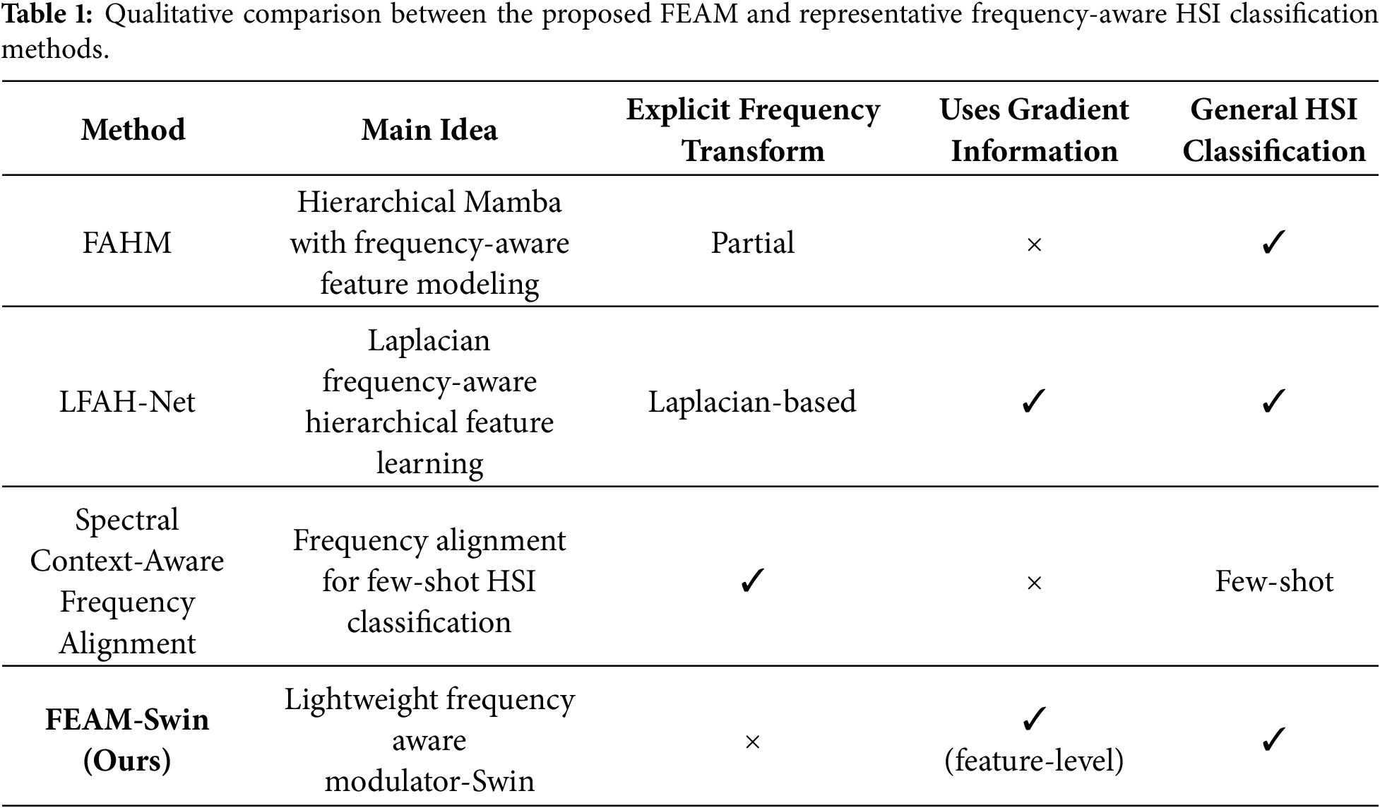
Recently, frequency-aware representation learning has emerged as an effective strategy for HSI classification. Representative approaches, such as FAHM [76], LFAH-Net [77], and Spectral Context-Aware Frequency Alignment [78], have demonstrated the effectiveness of incorporating frequency information into deep HSI classification models through hierarchical frequency modeling, Laplacian-based feature enhancement, and frequency alignment mechanisms. Although these methods have achieved promising performance, they generally rely on explicit frequency modeling strategies, handcrafted frequency operators, or task-specific architectural designs. A qualitative comparison is shown in Table 1. Consequently, designing a lightweight and general frequency-aware module that can be seamlessly integrated into hierarchical vision transformers remains an open challenge.

Although transformer-based methods have shown considerable effectiveness in HSI classification, several critical limitations have yet to be addressed. First, the self-attention (SA) mechanism employed in conventional Vision Transformer (ViT) encoders exhibits an inherent bias toward modeling global contextual dependencies. While this characteristic proves advantageous for capturing long-range spatial interactions, it frequently fails to preserve fine-grained local spectral–spatial variations with sufficient fidelity that are crucial for distinguishing spectrally similar materials in HSI analysis, particularly in scenarios characterized by limited training samples. Specifically, the absence of explicit mechanisms to emphasize localized spectral fluctuations and high-frequency spectral–spatial transitions results in suboptimal discriminative performance when classifying complex heterogeneous scenes.

Second, many contemporary transformer-based HSI classification models rely on sophisticated multi-stage tokenization strategies and deep encoder architectures to enhance feature representation capacity. Consequently, this design philosophy results in a substantial increase in both model parameterization and computational complexity, rendering such models highly susceptible to overfitting when training data are scarce, a pervasive challenge in real-world hyperspectral remote sensing applications. Although lightweight architectures have been explored in recent literature to mitigate these concerns, including compact Swin-based designs with squeeze-and-excitation or squeeze-and-expansion channel recalibration [79,80], a groupwise separable convolutional vision transformer [81], and state-space alternatives such as MorpMamba and DiMA [82,83], their simplified architectures often struggle to effectively capture and model the intricate spectral–spatial structures inherent to hyperspectral data, thereby leading to a degradation in classification accuracy and reduced generalization capability.

In contrast, the proposed FEAM-Swin framework directly addresses these limitations by introducing a novel lightweight Frequency-Enhanced Attention Modulator (FEAM) that is seamlessly integrated into a hierarchical Swin Transformer architecture. Unlike existing frequency-aware HSI classification methods that rely on explicit frequency-domain transformations, handcrafted frequency operators, or task-specific frequency modeling strategies, FEAM performs lightweight frequency-aware feature modulation directly on intermediate feature representations through gradient-based frequency energy estimation. Consequently, FEAM enhances local spectral–spatial discriminative information while preserving computational efficiency and avoiding costly attention mechanism redesigns or explicit Fourier and wavelet transforms. The main contributions of this paper are as follows:

1.   We propose FEAM-Swin, a novel lightweight Swin Transformer architecture that explicitly incorporates frequency-aware modeling for HSI classification. The proposed framework effectively balances long-range contextual dependency modeling and fine-grained spectral–spatial discrimination under strict computational constraints.

2.   A Frequency-Enhanced Attention Modulator (FEAM) is introduced to capture local spectral–spatial frequency variations via gradient-based energy estimation. Unlike conventional frequency-domain approaches, FEAM avoids explicit Fourier or wavelet transforms, achieving frequency-sensitive feature enhancement with minimal parameter and computational overhead.

3.   FEAM is seamlessly embedded within hierarchical Swin Transformer blocks, enhancing local discriminability while preserving the efficiency of window-based self-attention. This design strengthens frequency-aware representation learning without increasing architectural complexity or compromising scalability.

4.   We introduce a lightweight Dynamic Context Scaling mechanism that enhances the standard window-based self- attention by incorporating global contextual information into the attention score computation. DCS adaptively scales attention weights based on global context vectors derived from the attention matrix, enriching the model’s ability to capture long-range spectral dependencies without substantially increasing computational overhead.

5.   Extensive experiments on four benchmark HSI datasets demonstrate that FEAM-Swin consistently attains state-of-the-art classification performance in terms of overall accuracy, average accuracy, and Kappa coefficient, while maintaining lower model complexity compared with existing CNN and transformer-based methods.

The remainder of this paper is organized as follows. Section 2 details the proposed FEAM-Swin framework. Section 3 presents the experimental setup and quantitative performance evaluation. Finally, Section 4 concludes the paper and discusses future research directions.

2  Proposed Method

2.1 FEAM-Swin

In this section, we present the FEAM-Swin, a novel framework designed to enhance HSI classification by effectively capturing spatial and spectral dependencies while minimizing computational overhead. The overall architecture of the proposed FEAM-Swin is illustrated in Fig. 1, and the detailed information of the proposed architecture is given below.

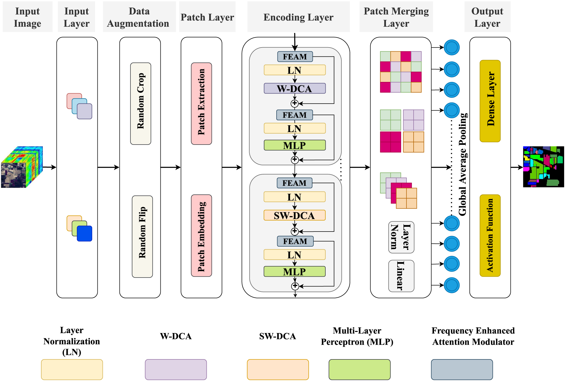
Figure 1: The architecture of the proposed FEAM-Swin model is structured to enhance feature representation and classification performance. Initially, the input undergoes data augmentation (random crop layers and random flip layers), patch extraction and embedding. This is followed by a series of normalization layers, Window Dynamic Context Attention mechanisms (W-DCA), Shifted Window Dynamic Context Attention (SW-DCA), and multilayer perceptrons (MLPs). To further refine feature representations, FEAM blocks are systematically integrated at each stage. Finally, the model applies global average pooling and subsequently uses fully connected layers to produce the classification results at the final output layer.

2.2 Overview of the Approach

The proposed FEAM-Swin framework is designed to achieve an effective balance between discriminative spectral–spatial representation learning and computational efficiency for HSI classification. Built upon the hierarchical Swin Transformer backbone, FEAM-Swin preserves the advantages of window-based self-attention for modeling long-range contextual dependencies, while introducing a lightweight FEAM to explicitly exploit frequency-sensitive cues that are critical for distinguishing spectrally similar land-cover classes.

Unlike conventional frequency-aware approaches that rely on explicit spectral transforms (e.g., Fourier or wavelet decompositions), FEAM adopts a gradient-based formulation to implicitly estimate local spectral–spatial frequency variations. This design enables seamless integration into transformer blocks with negligible parameter overhead and without disrupting the hierarchical feature learning process. The mathematical formulation of the proposed Frequency-Enhanced Attention Modulator (FEAM) is detailed in Section 2.3. Specifically, FEAM computes channel-wise spectral–spatial variation descriptors using gradient operators and applies a lightweight gating mechanism to adaptively recalibrate feature responses within each transformer stage.

2.3 Frequency-Enhanced Attention Modulator (FEAM)

The FEAM block, as shown in Fig. 2, Conventional channel attention mechanisms estimate channel importance using global average pooling, which primarily captures low-frequency (DC) responses while under-representing structural variations. To better characterize spatial–spectral discontinuities in hyperspectral feature maps, we construct a frequency-aware descriptor using discrete gradient operators.

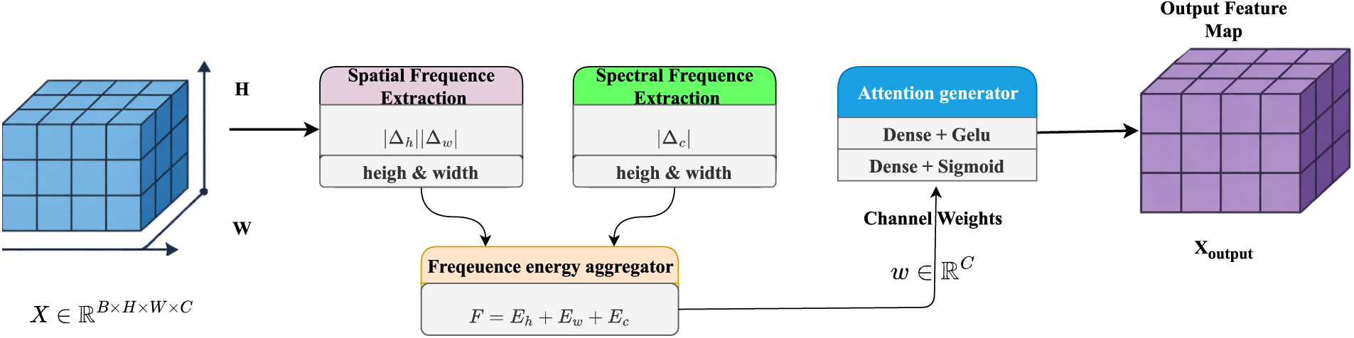
Figure 2: The Architecture of the FEAM block of our proposed FEAM-Swin method.

2.3.1 Gradient-Based Frequency Descriptor

To construct a frequency-aware representation of the input hyperspectral feature map, spatial and spectral gradient operators are applied to capture local variations along all three dimensions of the feature tensor. Let the input feature tensor be X∈RB×H×W×C, where B, H, W, and C denote batch size, spatial height, spatial width, and number of channels, respectively.

2.3.2 Spatial Gradients

To approximate first-order spatial derivatives, forward finite differences are employed along the height dimension. Eq. (1) computes the difference between vertically adjacent feature elements, effectively measuring how the feature responses change along the spatial height axis. This operation highlights abrupt transitions and structural discontinuities in the vertical direction, which correspond to high-frequency spatial content. By operating directly on the feature tensor without any learnable parameters, this Eq. (1) remains computationally lightweight while capturing meaningful local spatial variation. Note that we denote the height-direction gradient as Dx and the width-direction gradient as Dy, following the row-major (H,W) indexing of the feature tensor X∈RB×H×W×C, rather than the conventional Cartesian image-axis convention in which x denotes the horizontal direction and y the vertical direction. As illustrated in Fig. 2, the gradient along the height direction is given by

DxX(b,h,w,c)=X(b,h+1,w,c)−X(b,h,w,c),(1)

for h∈[0,H−2], and the gradient along the width direction is given by

DyX(b,h,w,c)=X(b,h,w+1,c)−X(b,h,w,c),(2)

for w∈[0,W−2], where Eq. (2) extends the forward finite difference operation to the horizontal spatial dimension, computing the difference between laterally adjacent feature elements along the width axis. This captures high-frequency variations in the horizontal direction, complementing the vertical gradient computed in Eq. (1). Together, these two spatial gradient operators provide a comprehensive characterization of local spatial frequency content within each feature channel, enabling the model to detect edges, boundaries, and fine-grained structural patterns that are critical for discriminating spectrally similar land-cover classes in hyperspectral imagery. Channel-wise spatial energies are defined as:

Ex[b,c]=1(H−1)W∑h=0H−2∑w=0W−1|Dx[b,h,w,c]|,(3)

To obtain a compact channel-wise representation of spatial frequency content, Eq. (3) aggregates the absolute values of the height-direction gradient across all spatial positions for each channel. Specifically, the mean absolute gradient magnitude is computed by averaging over all valid spatial locations, yielding a scalar energy value per channel per sample. This channel-wise energy descriptor Ex∈RB×C encodes the degree of vertical spatial variation present in each feature channel, providing a global summary of high-frequency structural activity along the height dimension. Channels with high Ex values correspond to feature maps exhibiting strong vertical spatial transitions, indicating regions of greater discriminative relevance.

Ey[b,c]=1H(W−1)∑h=0H−1∑w=0W−2|Dy[b,h,w,c]|(4)

where Eq. (4) computes the mean absolute gradient magnitude along the width direction for each channel. By averaging the horizontal gradient responses across all valid spatial positions, Ey produces a compact scalar descriptor per channel that quantifies the overall level of horizontal spatial frequency variation. The complementary nature of Ex and Ey ensures that the resulting descriptors jointly capture directional spatial frequency information across both spatial axes, providing a more complete characterization of local structural content than would be achievable through a single-direction gradient alone.

Ex,Ey∈RB×C(5)

where Eq. (5) formally states the output dimensionality of the spatial energy descriptors derived from Eqs. (3) and (4). Both Ex and Ey are condensed into compact tensors of shape B×C, collapsing the spatial dimensions through mean aggregation while retaining the channel dimension. This dimensionality reduction is essential for enabling efficient downstream processing, as it transforms the spatially distributed gradient information into a channel-wise summary that can be directly utilized by the subsequent gating mechanism.

2.3.3 Spectral Gradient

To capture inter-band variation, we compute forward spectral differences as:

DzX(b,h,w,c)=X(b,h,w,c+1)−X(b,h,w,c),(6)

for c∈[0,C−2]. Beyond spatial gradients, hyperspectral data also exhibits meaningful variation along the spectral dimension, as adjacent spectral bands often carry complementary and overlapping information. To capture inter-band spectral transitions, Eq. (6) applies a forward finite difference operator along the channel axis, computing the difference between spectrally adjacent feature responses at each spatial location. This spectral gradient highlights abrupt changes between neighboring spectral bands, which are indicative of high-frequency spectral content and are particularly informative for distinguishing materials with similar but subtly different spectral signatures. The inclusion of spectral gradient information distinguishes the proposed frequency descriptor from purely spatial attention mechanisms, enabling a more holistic frequency-aware characterization of hyperspectral features. The spectral energy is computed as:

Ez[b,c]=1HW∑h=0H−1∑w=0W−1|Dz[b,h,w,c]|(7)

To obtain a spatially aggregated representation of inter-band spectral variation, Eq. (7) computes the mean absolute spectral gradient magnitude across all spatial positions for each spectral channel. The resulting descriptor Ez quantifies the average degree of spectral transition between channel c and channel c+1 aggregated across all spatial positions, providing a compact measure of spectral frequency activity. Channels exhibiting high Ez values correspond to spectral regions characterized by rapid inter-band variation, which are typically associated with informative spectral features that facilitate accurate classification of spectrally complex land-cover types.

Ez∈RB×(C−1)(8)

where in Eq. (8), the spectral energy descriptor Ez has a reduced channel dimension of C−1 rather than C, arising directly from the forward finite difference formulation used in Eq. (6), which computes differences between adjacent channel pairs and therefore produces one fewer output than the number of input channels. While this reduced dimensionality accurately reflects the nature of the spectral gradient operation, it introduces a channel dimension mismatch that must be resolved before Ez can be combined with the spatial energy descriptors Ex and Ey.

To resolve the channel dimension mismatch in Eq. (8) and ensure compatibility with the spatial energy descriptors, Eq. (9) applies zero-padding to the last channel of Ez. Specifically, the spectral energy values for channels 0 through C – 2 are preserved exactly as computed, while a zero value is appended at position C – 1 to extend the descriptor to the full channel dimensionality C. This simple and parameter-free alignment strategy ensures that the spectral energy descriptor can be seamlessly combined with the spatial descriptors in subsequent aggregation steps without introducing any additional learnable parameters or computational cost.

E~z[b,c]={Ez[b,c],0≤c≤C−20,c=C−1(9)

Thus,

E~z∈RB×C(10)

The Eq. (10) confirms that the spectral energy descriptor E~z now shares the same dimensionality B×C as the spatial energy descriptors Ex and Ey defined in Eq. (5). This dimensional alignment is a prerequisite for the subsequent element-wise aggregation step described in Eq. (11), wherein all three descriptors are combined to form the final unified frequency descriptor E. The consistent tensor shape across all three descriptors ensures that the aggregation can be performed efficiently through simple element-wise addition, without the need for any reshaping, projection, or interpolation operations.

2.3.4 Final Frequency Descriptor

With compact channel-wise energy descriptors derived from both spatial and spectral gradient operations, the proposed FEAM module proceeds to aggregate these descriptors into a unified frequency representation, which is subsequently passed through a lightweight gating network to generate adaptive channel attention weights. The aggregated frequency descriptor is defined element-wise as:

E[b,c]=Ex[b,c]+Ey[b,c]+E~z[b,c](11)

The Eq. (11) defines the final aggregated frequency descriptor E, through element-wise summation of the three individually computed energy components: the height-direction spatial energy Ex,the width-direction spatial energy Ey, and the zero-padded spectral energy E~z. This additive aggregation strategy is deliberate and principled: by combining spatial and spectral frequency information into a single unified descriptor, the model captures a holistic characterization of local frequency activity across all three dimensions of the hyperspectral feature tensor. The element-wise summation preserves the channel-wise structure of each individual descriptor, with contributions from all three gradient directions equally represented at every channel except the last (c=C−1), where the spectral component is zero-padded per Eq. (9). This aggregation is entirely parameter-free, introducing no additional learnable weights and thus maintaining the computational efficiency that is central to the design approach of the proposed FEAM module. Channels with consistently high energy values across multiple gradient directions are indicative of spectrally and spatially active regions, and therefore assigned greater importance in the subsequent recalibration step.

E∈RB×C(12)

where Eq. (12) establishes the output dimensionality of the aggregated frequency descriptor E. As a direct consequence of the dimensional alignment achieved through zero-padding in Eq. (9) and the element-wise summation in Eq. (11), the final descriptor retains the compact shape of B×C, where B denotes the batch size and C denotes the number of feature channels. This compact representation is particularly significant from a computational point of view, as it reduces the full spatial–spectral feature tensor X∈RB×H×W×C to a channel-wise summary without any learnable compression operations. The resulting descriptor E thus serves as an efficient and informative bottleneck representation that encapsulates the frequency characteristics of each channel, providing a strong basis for the adaptive channel recalibration performed in the subsequent gating network.

2.3.5 Frequency Interpretation

For a continuous signal f(x), the Fourier transform of its derivative satisfies

ℱ{∂f(x)∂x}=jωℱ{f(x)}(13)

where ω denotes the angular frequency. Eq. (13) provides the theoretical justification for using gradient-based operations as a proxy for frequency-domain analysis. Specifically, this relationship derived from the differentiation property of the Fourier transform states that the Fourier transform of the first-order derivative of a continuous signal f(x) is equal to the product of jω and the Fourier transform of the original signal. The multiplicative factor jω scales each frequency component proportionally to its angular frequency ω, which has the direct effect of amplifying higher-frequency components relative to lower-frequency ones. This mathematical property formally establishes that derivative operators inherently act as high-pass filters in the frequency domain, emphasizing structural transitions, edges, and fine-grained variations that correspond to high-frequency content. In the context of the proposed FEAM module, this theoretical grounding confirms that the gradient-based spatial and spectral energy descriptors defined in Eqs. (1)–(11) effectively capture frequency-sensitive information without requiring explicit frequency-domain transforms such as Fourier or wavelet decompositions. This insight is central to the design of FEAM block, as it enables frequency-aware feature modulation through simple and computationally inexpensive finite difference operations, which scale linearly with the number of tensor elements rather than following the super-linear complexity of explicit spectral transform methods.

To provide a rigorous theoretical foundation in the discrete domain directly applicable to the discrete hyperspectral feature tensors processed by FEAM, we extend the above continuous-domain analysis to the discrete frequency setting. For a discrete feature map sequence x[n], the Discrete-Time Fourier Transform (DTFT) of its first-order forward finite difference satisfies:

ℱ{x[n+1]−x[n]}=(ejω−1)X(ejω)(14)

The magnitude of the frequency response of the finite difference operator is given by:

|ejω−1|=2|sin⁡(ω2)|(15)

This magnitude function is monotonically increasing for ω∈[0,π], confirming that finite difference operators amplify higher discrete frequencies relative to lower ones in discrete feature maps directly analogous to the continuous-domain high-pass filtering property established in Eq. (13). This result provides the discrete-domain theoretical justification for using finite difference operations as frequency-sensitive descriptors on hyperspectral feature tensors. Furthermore, the approximation error between the exact continuous derivative and the discrete finite difference operator is bounded by:

|∂f∂x−Δfh|≤h2max|∂2f∂x2|(16)

where h denotes the grid spacing, equal to 1 for unit-spaced feature map pixels. This bound confirms that finite differences provide a valid and accurate first-order approximation to the derivative operator on discrete feature maps, with the approximation error decreasing as the feature map resolution increases.

Additionally, the channel-wise gradient energy descriptor Ex[b,c] (Eq. (3)) aggregates the absolute gradient magnitudes across all spatial positions for each channel. This operation is equivalent to computing the L1 norm of the high-pass filtered feature map in the spatial domain. The L1 norm aggregation provides a robust, non-negative, translation-invariant, and computationally stable measure of high-frequency activity per channel. Unlike phase-sensitive Fourier coefficients, which require complex-valued arithmetic, explicit transform computation of complexity O(BHWC log(HW)), and inverse transforms for spatial-domain recovery, gradient magnitudes are entirely real-valued, parameter-free, and directly computable in a single forward pass with linear complexity O(BHWC). Furthermore, gradient magnitudes are invariant to spatial translation of feature patterns, providing a more compact and stable frequency energy estimate compared to raw Fourier coefficients whose phase components vary with spatial position. These theoretical properties collectively establish gradient magnitude aggregation as a principled, mathematically grounded, computationally efficient, and practically stable replacement for explicit Fourier or wavelet frequency decomposition in the context of channel-wise frequency energy estimation for hyperspectral feature recalibration.

2.3.6 Channel Recalibration

The frequency descriptor is passed through a two-layer gating network. The Eq. (17) defines the lightweight two-layer gating network responsible for transforming the aggregated frequency descriptor E into a set of adaptive channel attention weights w. The operation proceeds in two sequential stages. In the first stage, the frequency descriptor E is linearly projected into a lower-dimensional intermediate representation through multiplication with the weight matrix W1∈RC×Cr, where r denotes the channel reduction ratio. This dimensionality reduction serves a dual purpose, it compresses the channel-wise frequency information into a more compact latent space, and reduces the overall parameter count of the gating network, thereby preserving computational efficiency. The compressed representation is then passed through the GELU activation function δ(⋅), which introduces non-linearity and enables the network to model complex, non-linear relationships between frequency energy patterns and channel importance. In the second stage, the activated intermediate representation is projected back to the original channel dimensionality through multiplication with W2∈RCr×C, and a sigmoid activation function σ(⋅) is applied to normalize the output values to the range (0, 1). The resulting vector w contains a scalar attention weight for each channel, representing the relative importance of that channel based on its frequency energy characteristics.

w=σ(δ(EW1)W2)(17)

where

W1∈RC×Cr,W2∈RCr×C(18)

Eq. (18) explicitly defines the dimensions of the two learnable weight matrices W1 and W2 employed in the gating network of Eq. (17). The first projection matrix W1 maps the input frequency descriptor from the full channel space of dimension C to a compressed intermediate space of dimension Cr, where r is the reduction ratio hyperparameter that governs the degree of channel compression. A larger value of r results in a more aggressive compression, reducing the number of parameters in the gating network but potentially limiting its capacity to model fine-grained inter-channel frequency relationships. The second projection matrix W2 performs the inverse mapping, restoring the representation from the compressed space of dimension Cr back to the original channel dimensionality C, enabling the generation of a full channel-wise attention weight vector. This symmetric bottleneck structure ensures that the total number of additional parameters introduced by the FEAM gating network is 2C2r, which remains negligibly small relative to the overall model parameter count for practical values of r. This parameter efficiency is a key advantage of the proposed design, as it allows the FEAM module to be seamlessly integrated into each stage of the hierarchical Swin Transformer backbone without meaningfully increasing model complexity or computational overhead. The reduction ratio is set to r = 4, yielding an intermediate representation of dimension C/r = 16 for the default embedding dimension C = 64. This introduces only 2048 additional trainable parameters per FEAM block, representing a negligible overhead relative to the total model parameter count.

The Eq. (19) formally establishes the dimensionality of the channel attention weight matrix w produced by the gating network defined in Eq. (17). The weight tensor w has a shape of B×C, where B denotes the batch size and C denotes the number of feature channels. Each scalar entry w[b,c] represents the normalized attention weight assigned to channel c of the b-th sample in the batch, with values constrained to the range (0, 1) by the sigmoid activation function applied in Eq. (17). The channel-specific nature of w enables the subsequent recalibration step to selectively modulate individual feature channels based on their respective frequency energy characteristics, thereby enhancing the discriminative power of spectrally informative channels while suppressing those carrying low-frequency information. Importantly, the batch dimension in w allows the attention weights to be independently computed for each sample, ensuring that the recalibration adapts dynamically to the frequency content of individual input instances.

w∈RB×C(19)

Channel-wise recalibration is then performed as:

Y[b,h,w,c]=X[b,h,w,c]⋅w[b,c](20)

where Eq. (20) defines the core recalibration operation of the FEAM module, wherein the input feature tensor X is modulated by the channel attention weights w through element-wise multiplication. For each spatial location (h,w) and each channel c of the b-th sample, the corresponding feature response X[b,h,w,c] is scaled by the attention weight w[b,c], producing the recalibrated output feature Y[b,h,w,c]. This operation is applied uniformly across all spatial positions within each channel, meaning that the same attention weight governs the scaling of every spatial feature response belonging to a given channel. The recalibration mechanism is therefore spatially invariant but channel-selective, enabling the model to globally amplify feature channels that exhibit strong frequency activity while attenuating those dominated by low-frequency or spectrally uninformative content.

Y∈RB×H×W×C(21)

The Eq. (21) confirms that the recalibrated output feature tensor Y preserves the same spatial and spectral dimensionality as the input feature tensor X∈RB×H×W×C. This dimensional consistency is a fundamental property of the proposed recalibration operation, as it ensures that the FEAM module can be seamlessly inserted into any stage of the hierarchical Swin Transformer backbone without requiring any architectural modifications, additional reshaping operations, or resolution adjustments.

2.3.7 Shifted Window Dynamic Context Attention

Let a window contain N tokens and Ha attention heads, with per-head dimension defined as

dh=CHa(22)

For each head, the query, key, and value projections satisfy

Qh,Kh,Vh∈RBw×N×dh(23)

where Bw denotes the number of windows. Attention is then computed as

Attention(Qh,Kh,Vh)=AVh,where A=Softmax(QhKh⊤dh)(24)

While window attention effectively models local, within-window contextual relationships (with cross-window context introduced via the shift in SW-DCA), it does not explicitly emphasize high-frequency variations. The proposed frequency-aware recalibration module therefore enhances structural sensitivity and complements transformer-based feature modeling.

2.3.8 Dynamic Context Scaling

While conventional self-attention relies solely on the pairwise interactions captured in A, the dynamic context scaling (DCS) mechanism introduces an adaptive factor that modulates these scores based on global contextual information. The key idea is to aggregate the attention scores within each window to form a context vector, which is then used to scale the original attention scores.

For each window, the context vector C is computed by averaging the attention scores across the spatial dimensions. Denoting the ith row of the attention matrix A (corresponding to the ith token) as Ai, the context vector is defined as:

C=1w2∑i=1w2Ai.(25)

This vector encapsulates the average attention behavior within the window, representing the global context. The computed context vector C is then used to scale the attention scores in an element-wise manner:

Ascaled=A⊙C,(26)

where ⊙ denotes row-wise broadcasted element-wise multiplication: the length-w2 context vector C is broadcast across every row of the w2×w2 attention matrix A, i.e., Ascaled[i,:]=A[i,:]⊙C for each row i=1,…,w2. This operation enhances the attention scores for tokens deemed globally important while suppressing less significant ones. After applying dynamic scaling, the scaled attention scores are normalized via the softmax function along the token dimension:

Asoftmax=softmax(Ascaled).(27)

To further enable cross-window interaction and enhance global contextual modeling, the proposed W-DCA is extended to a Shifted Window Dynamic Context Attention (SW-DCA) mechanism. In SW-DCA, the window partitioning is spatially shifted by half the window size along both spatial dimensions before applying the same dynamic context attention process. This shifting strategy allows tokens near window boundaries to attend to neighboring windows, thereby facilitating information exchange across windows while preserving the computational efficiency of window-based attention.

The final output of the attention mechanism for the window is obtained by weighting the value vectors V with the normalized scores:

O=AsoftmaxV.(28)

This output O is subsequently passed through an additional linear projection and dropout before being integrated with residual connections in the overall network architecture.

To further enhance the quality of feature representations extracted by the attention mechanism, a Multilayer Perceptron (MLP) is employed. The MLP serves as a fundamental component of the model, comprising multiple fully connected layers, with a Gaussian Error Linear Unit (GELU) activation function applied after the first linear transformation. This architectural design enables the model to capture complex, nonlinear dependencies within the input data, facilitating the learning of intricate patterns that cannot be effectively represented through linear transformations alone. The mathematical formulation of the MLP is defined as follows:

MLP(x)=U2⋅GELU(U1⋅x+b1)+b2(29)

where U1 and U2 denote learnable weight matrices, b1 and b2 represent bias vectors, and GELU functions as the activation mechanism. Compared to traditional activation functions such as ReLU, GELU [84] has demonstrated superior efficacy in deep learning applications by ensuring smoother gradient propagation and enhancing the model’s capacity to extract informative features. The MLP plays a crucial role in capturing high-level abstractions from raw input data, thereby transforming the feature space into a more discriminative representation. This advanced feature extraction is particularly advantageous in the context of HSI classification, where distinguishing between various spectral classes is critical for accurate analysis.

In addition to the MLP, the FEAM-Swin further enhances its representational power by integrating the FEAM mechanism. The FEAM block dynamically adjusts feature responses by modeling channel-wise dependencies, thereby improving the model’s sensitivity to salient features. A detailed discussion of the FEAM mechanism and its integration within the framework is provided in Section 2.3.

2.3.9 Patch Operations

Patch operations play a crucial role in the efficient processing of high-dimensional hyperspectral data by enabling localized feature extraction and structured representation through patch partitioning and embedding. The process begins with the Patch Extraction layer, which segments the input HSI into smaller, non-overlapping patches while preserving local spectral characteristics. These segmented patches are then mapped into a higher-dimensional latent space through the Patch Embedding layer.

The Patch Embedding operation transforms each patch into a structured high-dimensional representation, effectively capturing spectral information in a format suitable for subsequent processing. This transformation is essential for enhancing the spectral representation of each patch, thereby facilitating downstream tasks such as classification and segmentation [48]. To further refine these representations and improve information aggregation, the Patch Merging operation is applied. This step consolidates embeddings from adjacent patches, integrating their spectral information into a unified representation. The mathematical formulation of Patch Merging is given by:

xmg=Concat(xemb(i,j),xemb(i+1,j),xemb(i,j+1),xemb(i+1,j+1))W(30)

where xmg represents the merged feature vector, which aggregates embeddings (xemb) from neighboring patches in the image grid, including positions (i,j), (i+1,j), (i,j+1), and (i+1,j+1). The function Concat(⋅) performs a concatenation operation, combining these embeddings into a single vector. This concatenated feature vector is subsequently projected into a new feature space using the learnable weight matrix W.

By integrating neighboring embedded patches and applying a linear transformation, the patch merging operation constructs a cohesive representation that incorporates both local spectral details and broader contextual information. This hierarchical approach not only reduces the spatial dimensionality of the data but also enhances spectral feature extraction, significantly improving the model’s ability to process and analyse high-dimensional HSIs with greater efficiency and accuracy.

2.3.10 Prediction Computation and Output Layer

The final layer of the proposed FEAM-Swin network is responsible for producing class predictions for each pixel in the HSI. Following the final transformer stage, global average pooling is applied across the spatial dimensions to obtain a compact feature vector, which is then passed to a fully connected (dense) layer that maps the extracted features to K predefined classes. The output of this layer is subsequently processed by a softmax activation function, transforming the raw scores into a probability distribution over the K classes. Mathematically, the output layer is defined as

Output(x)=softmax(Wout⋅x+bout)(31)

where x∈Rd denotes the input feature vector from the final transformer block (d being the embedding dimension of that stage), Wout∈Rd×K represents the weight matrix of the output layer, and bout∈RK is the associated bias vector. The softmax function is applied element-wise to normalize the logits into a probability distribution:

softmax(zi)=ezi∑j=1Kezj(32)

where zi represents the raw score (logit) for class i, and the denominator ensures normalization across all K classes. This transformation guarantees that the output values are non-negative and sum to one, thereby enabling a probabilistic interpretation of the model’s predictions.

The final classification output is represented as a prediction map Y∈{1,…,K}H×W, where each pixel is assigned to the class with the highest probability. If required, upsampling techniques such as transposed convolution can be applied to restore the classification output to match the original spatial resolution of the input HSI. This output layer serves as a crucial component in converting the extracted spectral features into discrete class labels, ensuring accurate classification of hyperspectral data.

2.3.11 Computational Complexity

The gradient computations in (1)–(6) each scale linearly with the number of tensor elements. Therefore, the overall computational complexity of the proposed module is given by:

𝒪(BHWC),(33)

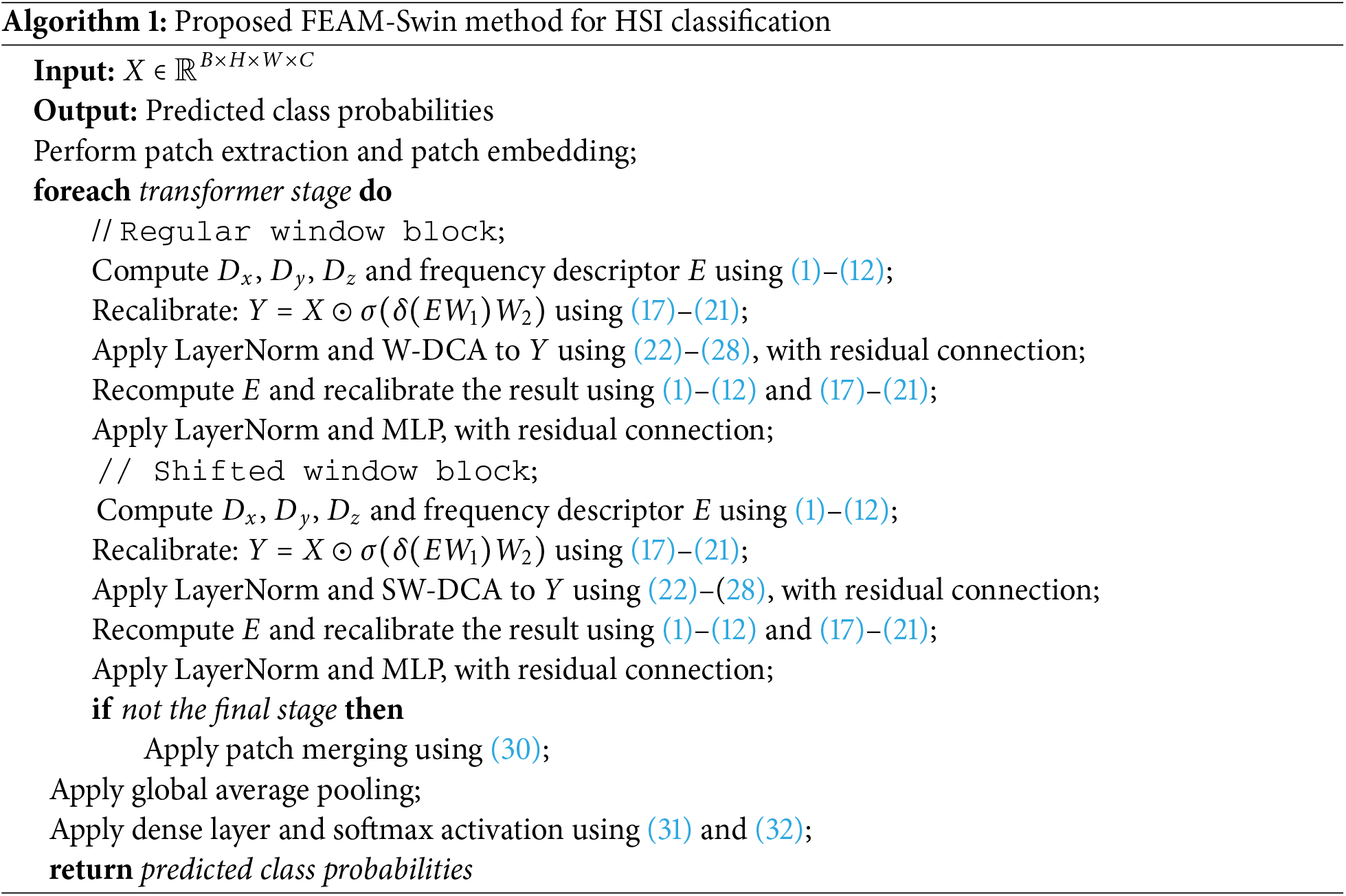
By temporarily expanding the channel dimensionality, the FEAM Block captures richer and more complex interdependencies between spectral bands. This is especially beneficial for hyperspectral data, where subtle variations across bands are crucial for class differentiation. Unlike traditional recalibration methods that merely reduce and restore channel dimensions, the FEAM Block enriches the feature representations, improving the separability between classes. As a result, the FEAM Block enhances the model’s ability to leverage the spectral richness of HSIs while reducing redundancy, leading to improved classification performance. Algorithm 1 summarizes the complete processing pipeline of the proposed Feam-Swin framework.

3  Experimental Evaluation

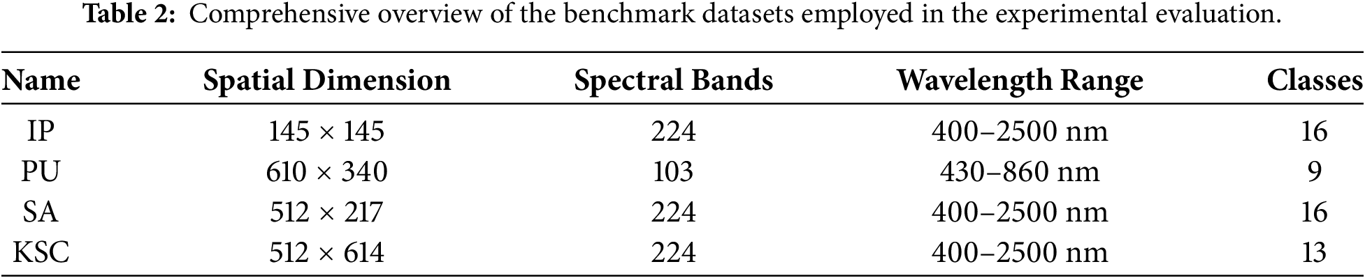
To comprehensively evaluate the proposed FEAM-Swin framework, experiments were conducted on four widely-used HSI benchmark datasets that cover diverse geographical regions, land-cover types, spatial resolutions, and imaging conditions (https://ieee-dataport.org/documents/hyperspectral-remote-sensing-scenes). Indian Pines (IP), University of Pavia (PU), Salinas (SA), and Kennedy Space Center (KSC). We first describe the experimental setup adopted in this study, including the configuration used for evaluation. This is followed by a detailed account of the hyperparameter settings employed in the proposed method, along with the corresponding experimental results. Subsequently, we provide a comprehensive comparison between our approach and existing state-of-the-art techniques. In addition, the influence of key hyperparameters is examined through systematic experiments and visual analyses. Overall, this framework is designed to offer a clear understanding of the effectiveness of the proposed method and its suitability for HSI analysis.

3.1 Datasets for Empirical Evaluation

In this section, we evaluate the performance of the proposed FEAM-Swin approach using four widely recognised hyperspectral datasets. These datasets are selected due to their importance and frequent use in HSI classification research. Each dataset includes raw HSIs and corresponding ground truth annotations, enabling a comprehensive assessment of classification accuracy and model effectiveness. Visual representations of the datasets are provided in Figs. 3–6.

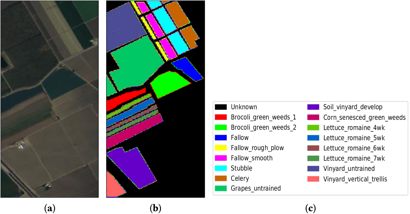
Figure 3: Visual representation of the SA dataset: (a) Original image, (b) Ground truth map, (c) Class legend.

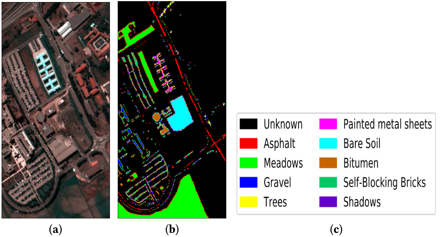
Figure 4: Visual representation of the PU dataset: (a) Original image, (b) Ground truth map, (c) Class legend.

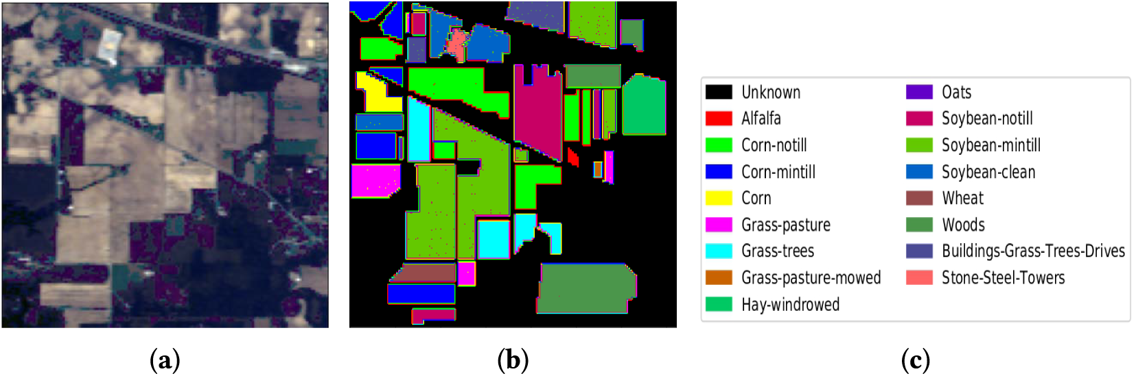
Figure 5: Visual representation of the IP dataset: (a) Original image, (b) Ground truth map, (c) Class legend.

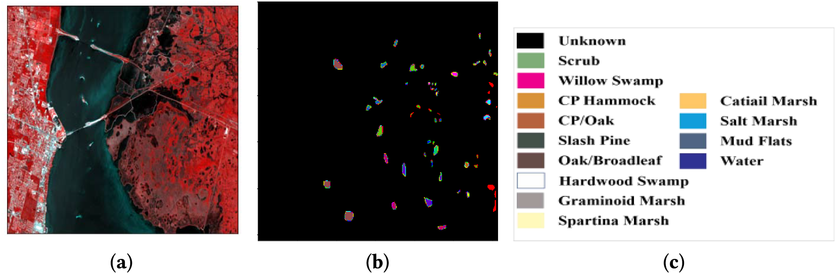
Figure 6: Visual representation of the KSC dataset: (a) Original image, (b) Ground truth map, (c) Class legend.

1.    The first dataset, referred to as SA, was acquired using the Airborne Visible/Infrared Imaging Spectrometer (AVIRIS) during a remote sensing survey of the Salinas Valley region in California, USA. This dataset boasts a high spatial resolution of 3.7 m per pixel, facilitating precise spectral analysis. It encompasses 224 spectral bands covering a broad wavelength range from 400 to 2500 nm, enabling the detection of subtle spectral variations among different materials. With spatial dimensions of 512×217 pixels, as summarized in Table 2, the dataset includes 16 distinct land cover classes, representing a diverse spectrum of agricultural elements such as vegetable crops, vineyard fields, and bare soil. These classifications play a pivotal role in applications related to precision agriculture and environmental monitoring. Furthermore, Table 3 provides a detailed breakdown of the class distribution alongside the corresponding training and testing datasets, offering valuable insights into the dataset’s structure and its potential utility for subsequent analytical studies.

2.    The second dataset, designated as PU, was acquired using the Reflective Optics Spectrographic Imaging System over Pavia, Italy, in 2002 via an airborne platform operated by the German Aerospace Center (DLR). This project was overseen by the German Aerospace Center under the HySens initiative, with funding provided by the European Union. Following the exclusion of 12 noisy spectral channels, the dataset comprises 610×340 pixels, each with a spatial resolution of 1.3 m per pixel. It encompasses 103 spectral bands spanning wavelengths from 430 to 860 nm, as detailed in Table 2. The data is partitioned into nine distinct classes, each representing various land cover types within the region. A comprehensive summary of the characteristics and specifications of these classes is provided in Table 4, offering valuable insights into the dataset’s applicability for remote sensing and environmental analysis.

3.    The third dataset employed in this paper is the Purdue Indiana Indian Pines scene (IP). Collected from the Indian Pines testing site in northwestern Indiana, this dataset features a spatial resolution of 20 m per pixel and covers an area of 145×145 pixels. It comprises 224 spectral bands that span wavelengths from 400 to 2500 nm, thus offering a comprehensive representation of the electromagnetic spectrum. The ground truth annotations consist of 16 distinct classes, each corresponding to various crops at different stages of growth, which reflects the region’s agricultural diversity. Detailed information regarding these classes is provided in Tables 2 and 5, underscoring the dataset’s relevance for applications in precision agriculture and remote sensing.

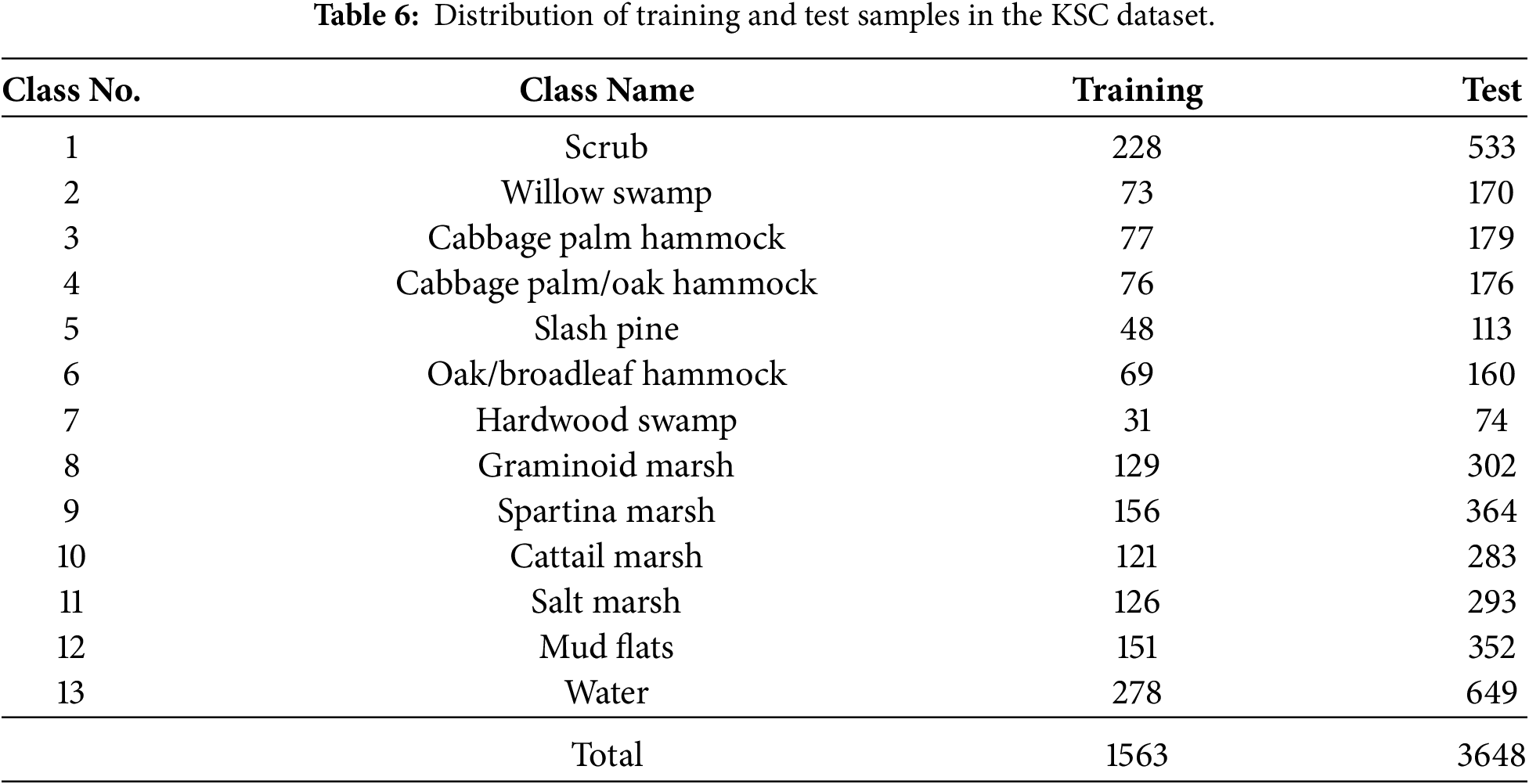
4.    The final dataset analyzed in this paper is the KSC dataset, acquired in 1996 using the AVIRIS sensor. Covering wavelengths from 400 to 2500 nm, this dataset enables detailed spectral analysis of the region. The corresponding image comprises 512×614 pixels and includes 224 spectral bands, as summarized in Table 2. Furthermore, the dataset includes 5211 labeled samples that are categorized into 13 distinct classes representing both upland and wetland environments. A comprehensive overview of these classes is provided in Table 6.

3.2 Experimental Setup

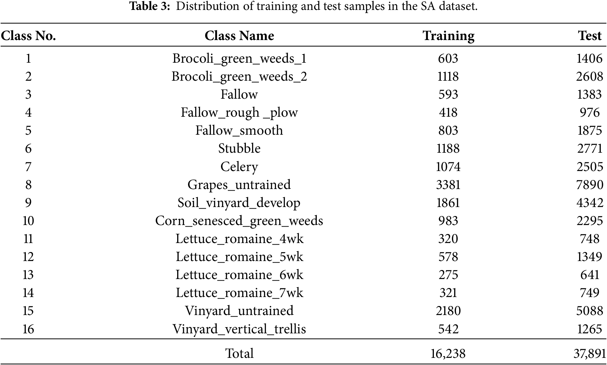
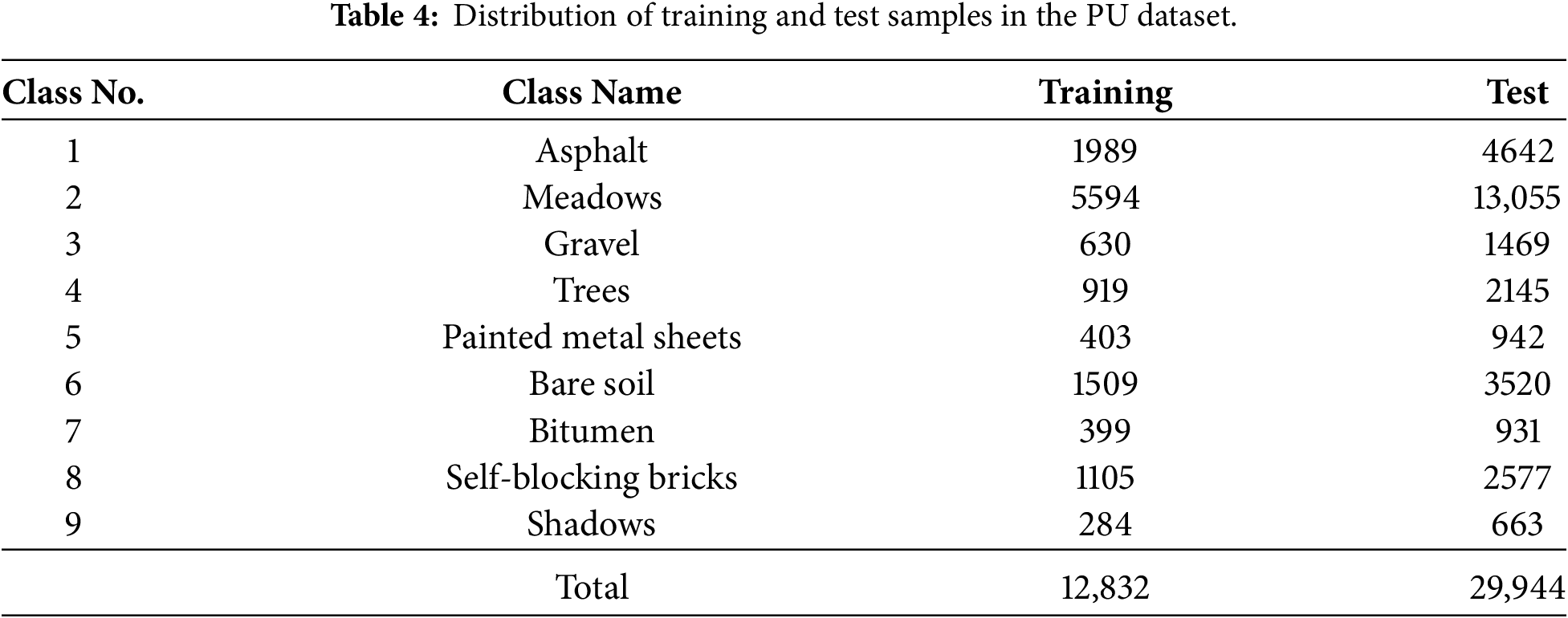
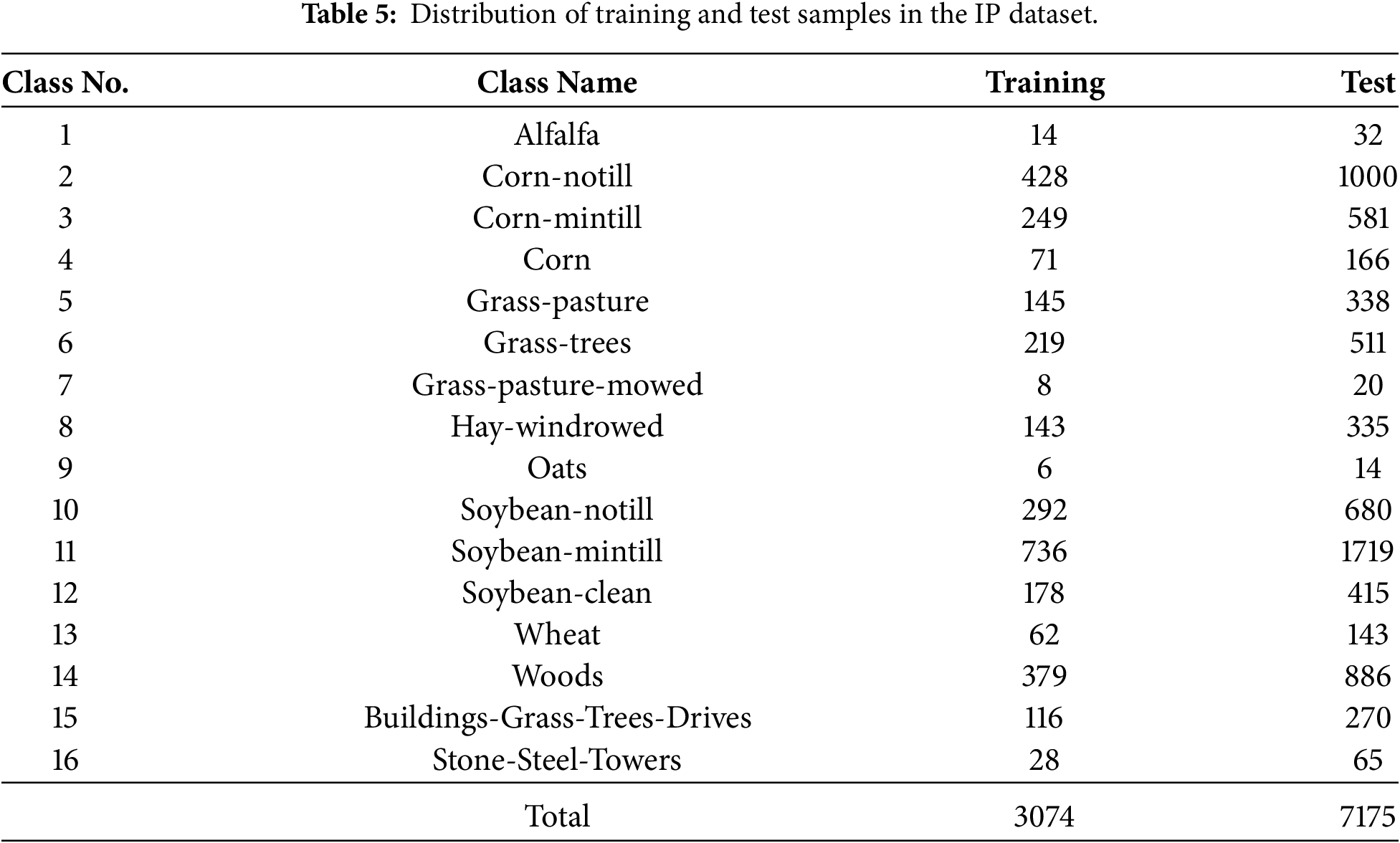
To assess the effectiveness of our proposed FEAM-Swin model, we conducted a comparative study against several SOTA techniques, including DiMA [83], MorpMamba [82], SwinT [56], PyFormer [55], PMCN [59], WaveFormer [60], and ViT [54], as well as traditional methods such as SVM-RBF (https://www.csie.ntu.edu.tw/cjlin/libsvm/), CCF-200 (https://github.com/twgr/ccfs), 2D CNN [37], GCNN [33], FADCNN [40], and NL-GCNN [32]. The code will be released upon acceptance of this paper (https://github.com/farhanmarwat). All experiments were performed on an NVIDIA RTX 4070 GPU (12 GB VRAM), with the host system equipped with 64 GB of RAM, to satisfy the computational requirements.

The model was implemented using the TensorFlow framework with an input shape of (25, 25, 30), representing the patch dimensions and the number of PCA components of the hyperspectral data. Designed for classification, the network produces outputs via layers containing 16 units (used for both the IP and SA datasets, each with 16 classes), 13 units (KSC), and 9 units (PU), corresponding to each dataset’s class count. The architecture incorporates a patch size of (2, 2) and applies a dropout rate of 0.03 to mitigate overfitting. Key hyperparameters include a learning rate of 1e–3, a batch size of 1024. Regarding the data partitioning protocol, 30% of the total available labeled samples were allocated to the combined training and validation pool, with the remaining 70% reserved exclusively for testing. Within the training pool, a validation split ratio of 0.1 was applied, reserving 10% of the training pool (approximately 3% of the total dataset) for model selection and early stopping, while the remaining 90% of the training pool (approximately 27% of the total dataset) was used for weight optimization. This partitioning strategy ensures a rigorous and unbiased evaluation by preventing any overlap between training, validation, and test subsets. The network configuration further specifies 8 attention heads, an embedding dimension of 64, and an MLP size of 256, with optimization conducted via AdamW at a weight decay of 0.0001. The loss criterion adopted is categorical cross-entropy, incorporating a label smoothing factor of 0.1. The FEAM gating network employs a channel reduction ratio of r = 4, compressing the frequency descriptor from dimension C = 64 to C/r = 16 in the intermediate representation before restoring it to the full channel dimensionality via sigmoid activation. This value was selected through a preliminary grid search over r∈2,4,8,16 based on validation performance on all the datasets. The training process spans 100 epochs to achieve optimal performance.

The evaluation metrics selected for this study provide a comprehensive quantitative comparison among various HSI classification methods. Detailed descriptions of each metric are provided below.

1.   Overall Accuracy (OA): OA is a core evaluation metric used to assess how well HSI classification methods perform. It is calculated by dividing the number of correctly classified test samples by the total count of test samples, offering a straightforward measure of how effective a given classification approach is.

2.   Average Accuracy (AA): AA is used to assess classification performance at the individual class level. It is derived by calculating the accuracy for each class separately and then computing the mean of those values. This makes AA a useful metric for understanding how consistently a method performs across all classes, rather than just in aggregate.

3.   Kappa Coefficient (κ): The κ is a well-established statistical measure used in HSI to evaluate classification reliability by accounting for agreement that may occur by chance alone. It captures the degree of correspondence between predicted and ground-truth class labels, making it a robust indicator of both the validity and consistency of the classification results.

3.3 Experimental Results and Discussion

Fig. 7 presents the convergence behavior of several Transformer-based models, including the proposed FEAM-Swin, by tracking accuracy and loss trends throughout training. Evaluations were conducted on four benchmark datasets SA, PU, IP, and KSC, where each model was trained for 100 epochs with an 2×2 patch size. The data was partitioned such that 30% of the total labeled samples were allocated to the training and validation pool (with an internal 90/10 training-validation split), while the remaining 70% served exclusively as the test set. To ensure a rigorous assessment of generalizability, careful partitioning was applied to prevent any overlap between the training, validation, and test subsets.

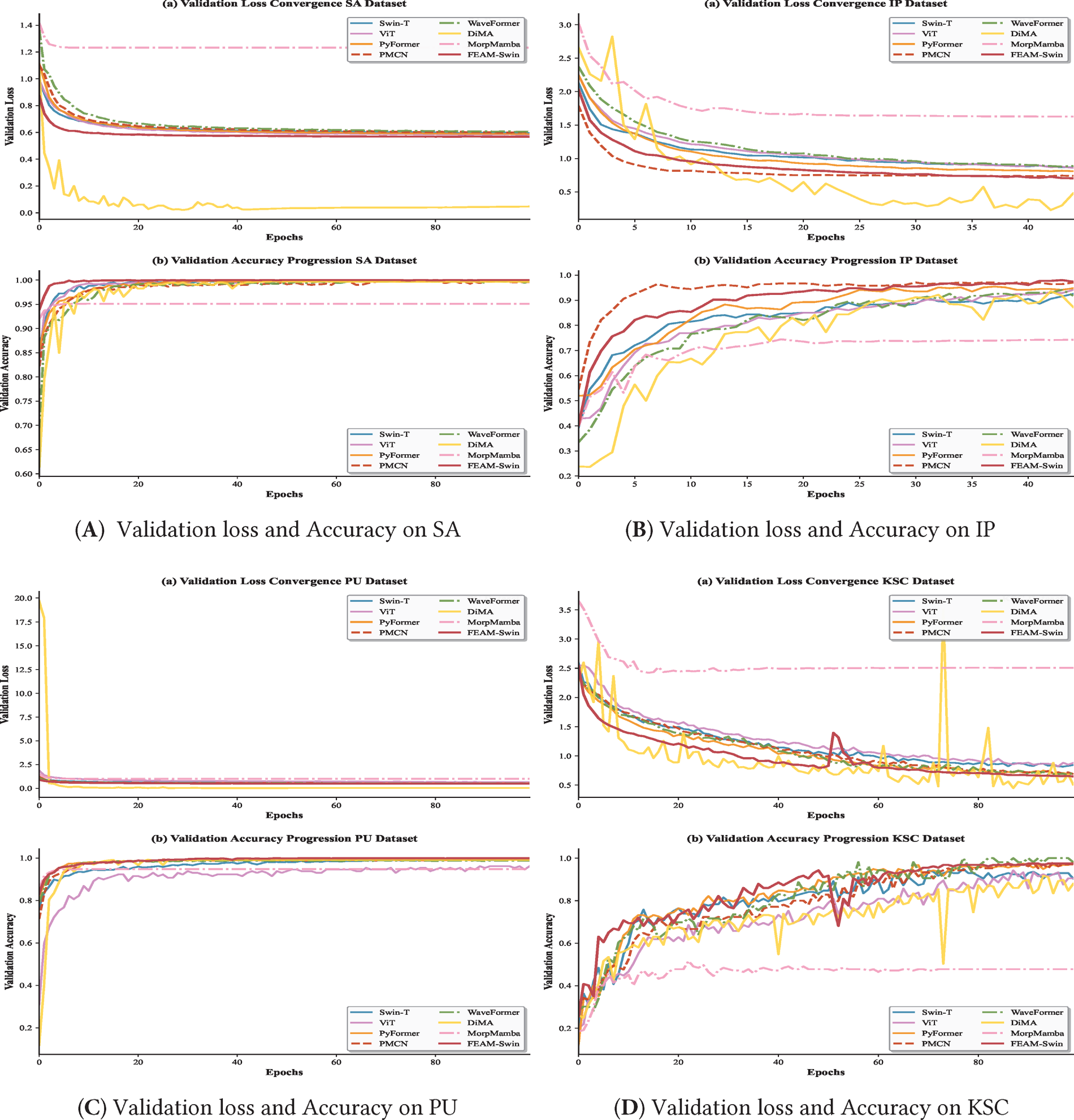
Figure 7: Training loss (top row) and classification accuracy (bottom row) curves of the proposed FEAM-Swin and five state-of-the-art Transformer-based methods on the SA, IP, PU, and KSC datasets. FEAM-Swin consistently achieves faster convergence and higher final accuracy across all datasets.

The effectiveness of the proposed FEAM-Swin approach is demonstrated through comprehensive experiments across multiple hyperspectral datasets, with performance measured using OA, AA, and κ. A comparison of these metrics reveals a clear progression in classification capability across different method generations. Conventional approaches such as SVM-RBF and CCF-200 show notably lower performance, while early CNN-based models, despite advancing beyond classical techniques, still struggle with the complex spectral-spatial characteristics of hyperspectral data. More recent Transformer-based architectures, including DiMA, WaveFormer, PMCN, PyFormer, and SwinT, achieve considerably stronger results, with OA typically ranging from the low 90s on the more heterogeneous IP and KSC datasets up to 99%+ on SA and PU. Among all evaluated methods, FEAM-Swin consistently attains the highest OA and AA across all four datasets (OA: 98.17%–99.97%; AA: 97.57%–99.95%), with near-perfect scores on SA, PU, and KSC and slightly lower but still leading performance on the more heterogeneous IP dataset, reflecting its capacity to extract and leverage fine-grained spectral information.

Taking the SA dataset as an example, traditional methods such as SVM-RBF and CCF-200 produce relatively modest OA scores of 88.82% and 89.72%, respectively, with AA values falling between 94.67% and 95.43% and κ that remain under 88.6%. Transformer-based architectures mark a significant leap in performance, with WaveFormer recording an OA of (OA = 99.40%, AA = 99.29%, κ = 99.33%), followed by PMCN (OA = 99.61%, AA = 99.59%, κ = 99.57%), PyFormer (OA = 99.75%, AA = 99.71%, κ = 99.72%), SwinT (OA = 99.88%, AA = 99.80%, κ = 99.87%), MorpMamba (OA = 95.01%, AA = 97.21%, κ = 94.44%), and DiMA (OA = 99.72%, AA = 99.72%, κ = 99.69%) for OA, AA, and κ, respectively. FEAM-Swin surpasses all of these, achieving an OA of 99.97%, AA of 99.95%, and κ of 99.96%, as shown in Table 7. This steady upward trend in performance underscores the value of the dynamic mechanisms embedded in FEAM-Swin, which equip it with the ability to distinguish between subtle class boundaries with exceptional accuracy, as further confirmed by the classification maps in Fig. 8.

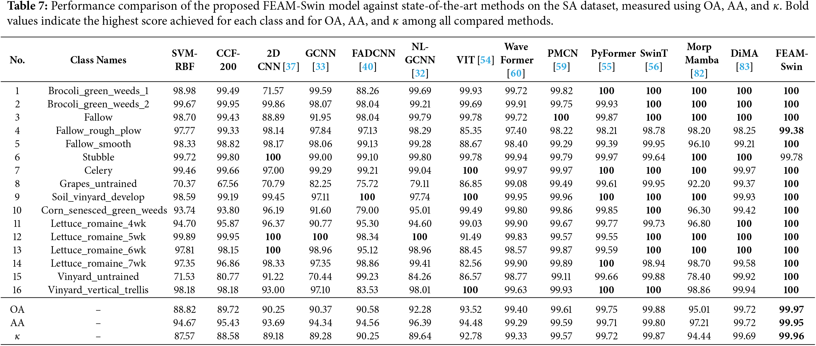
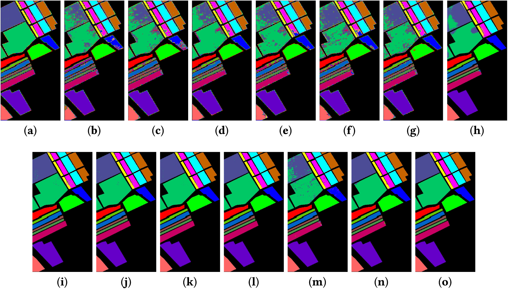
Figure 8: Classification maps generated by different methods on the SA dataset are displayed sequentially. (From Left to Right) (a) groundtruth, (b) SVM-RBF, (c) CCF-200, (d) 2-D CNN [37], (e) GCNN [33], (f) FADCNN [40], (g) NL-GCNN [32], (h) ViT [54], (i) WaveFormer [60], (j) PMCN [59], (k) PyFormer [55], (l) SwinT [56], (m) MorpMamba [82], (n) DiMA [83], and (o) (Proposed Approach) FEAM-Swin.

As illustrated in Table 8, the IP dataset presents a particularly demanding classification scenario due to the wide variety and complexity of its land cover categories, and it is here that FEAM-Swin’s strengths become most apparent. Traditional methods struggle considerably, with SVM-RBF and CCF-200 achieving OAs of only 74.24% and 82.87%, respectively, while early CNN-based models reach approximately 90.25% OA. More sophisticated CNN architectures such as FADCNN push this figure up to 97.80%, and other Transformer-based approaches yield further gains. Nevertheless, FEAM-Swin outperforms all competing methods by attaining an OA of 98.17%, an AA of 97.57%, and a κ of 97.91%. These findings demonstrate that FEAM-Swin’s architectural design allows it to maintain strong generalization even when confronted with highly heterogeneous and spectrally complex data distributions, as visualized in the classification maps of Fig. 9.

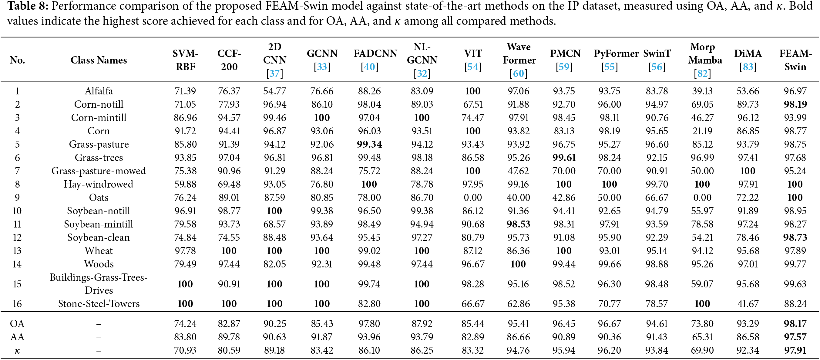
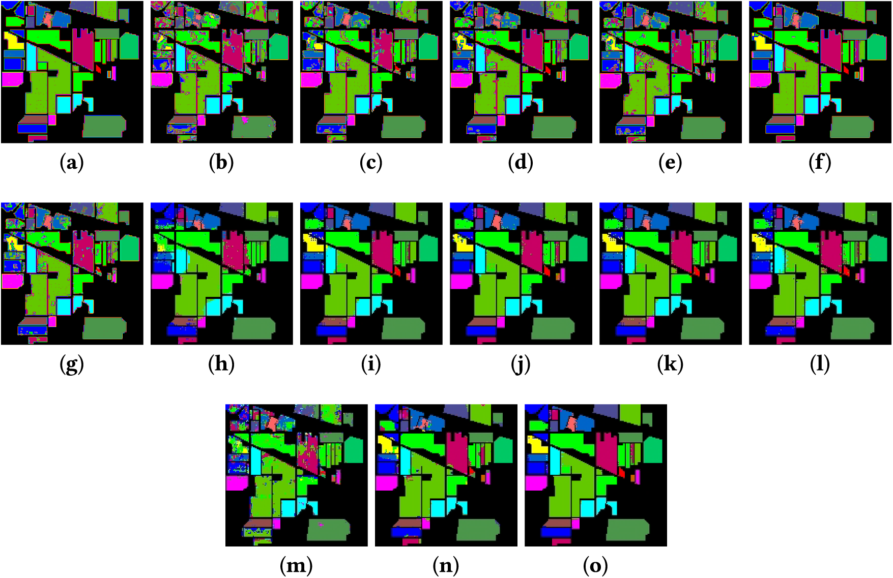
Figure 9: Classification maps generated by different methods on the IP dataset are displayed sequentially. (From Left to Right and from top to bottom) (a) ground-truth, (b) SVM-RBF, (c) CCF-200, (d) 2-D CNN [37], (e) GCNN [33], (f) FADCNN [40], (g) NL-GCNN [32], (h) ViT [54], (i) WaveFormer [60], (j) PMCN [59], (k) PyFormer [55], (l) SwinT [56], (m) MorpMamba [82], (n) DiMA [83], and (o) (Proposed Approach) FEAM-Swin.

A comparable performance trend emerges on the PU dataset, as shown in Table 9. Conventional methods such as SVM-RBF and CCF-200 yield OAs of 78.89% and 83.36%, respectively, while the weakest CNN baseline (2D CNN) reaches only 86.93% OA. Transformer-based models such as DiMA 99.11%, WaveFormer 98.90%, PMCN 99.04%, and PyFormer 99.06% push classification performance into the upper 98%–99% range, with SwinT reaching 99.41% OA; MorpMamba trails this group at 94.03% OA. FEAM-Swin builds on these gains and achieves an OA of 99.87%, an AA of 99.87%, and a κ of 99.83%, surpassing all competing approaches. The fact that such high scores are maintained even across particularly challenging classes confirms FEAM-Swin’s capacity to effectively handle complex spectral variations and class distribution imbalances, as shown in the classification maps of Fig. 10.

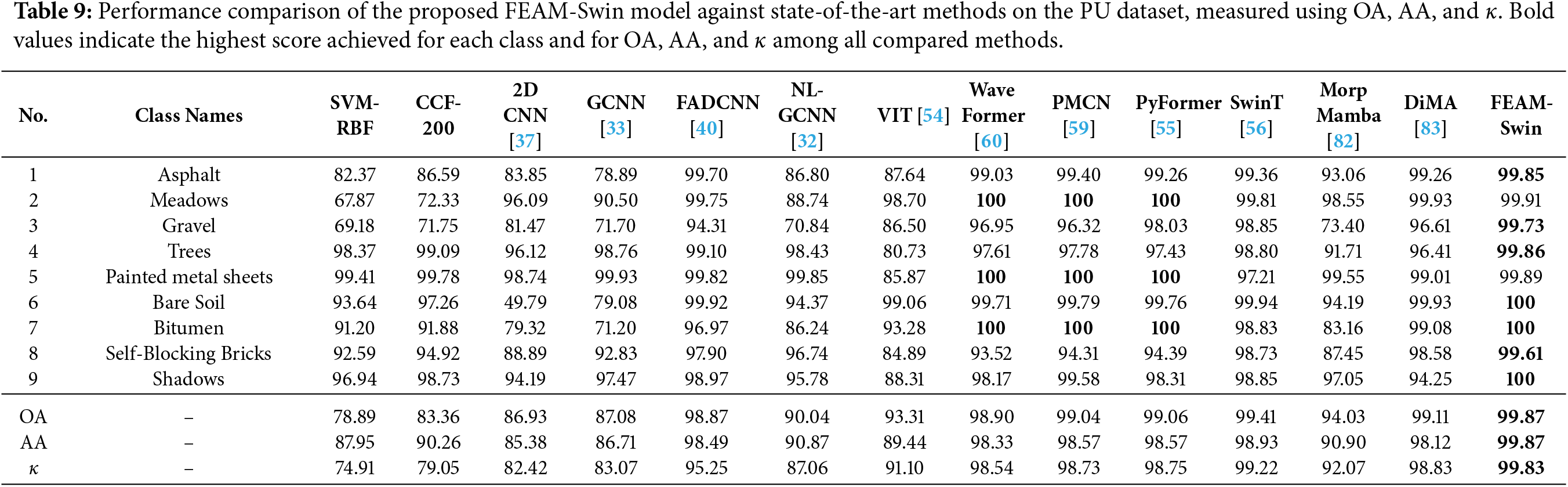
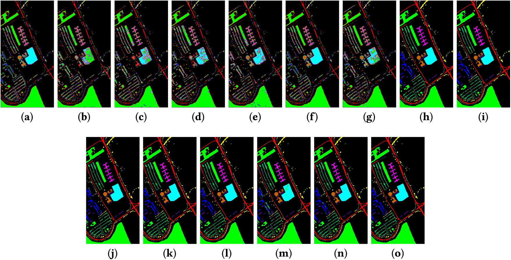
Figure 10: Classification maps generated by different methods on the PU dataset are displayed sequentially. (From Left to Right) (a) ground truth, (b) SVM-RBF, (c) CCF-200, (d) 2-D CNN [37], (e) GCNN [33], (f) FADCNN [40], (g) NL-GCNN [32], (h) ViT [54], (i) WaveFormer [60], (j) PMCN [59], (k) PyFormer [55], (l) SwinT [56], (m) MorpMamba [82], (n) DiMA [83], and (o) (Proposed Approach) FEAM-Swin.

The KSC dataset poses one of the greatest classification challenges due to the high degree of spectral similarity between its land cover classes, yet FEAM-Swin continues to deliver superior results. Traditional methods such as SVM-RBF and CCF-200 produce OAs of only 78.53% and 83.81%, respectively, and CNN-based models similarly fall short, failing to surpass the 90% OA threshold. Transformer-based architectures bring notable improvements, with methods like WaveFormer, PyFormer exceeding 96% OA. Despite these advances, FEAM-Swin outperforms them all, recording an OA of 98.41%, an AA of 98.28%, and a K of 98.22%, as illustrated in Table 10. These outcomes highlight FEAM-Swin’s strong discriminative capability, demonstrating its ability to accurately separate classes even when their spectral signatures are closely resembling one another, as exhibited in the classification maps of Fig. 11.

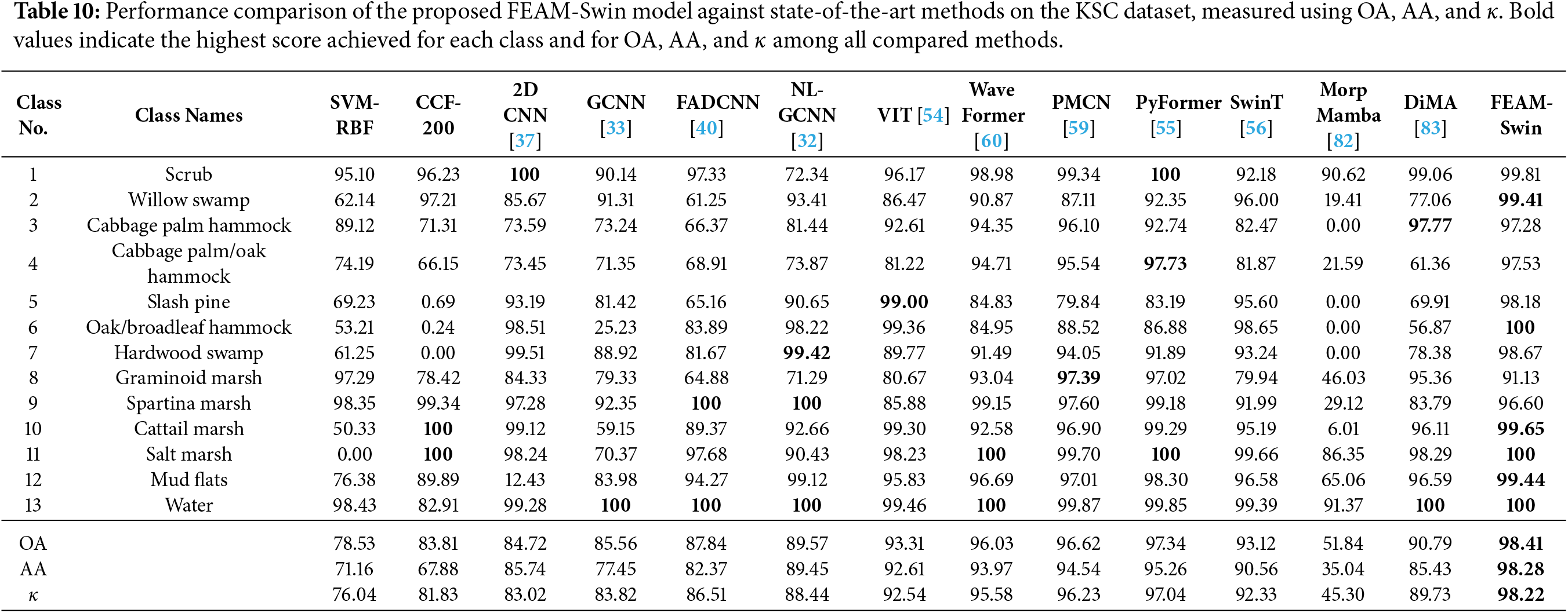
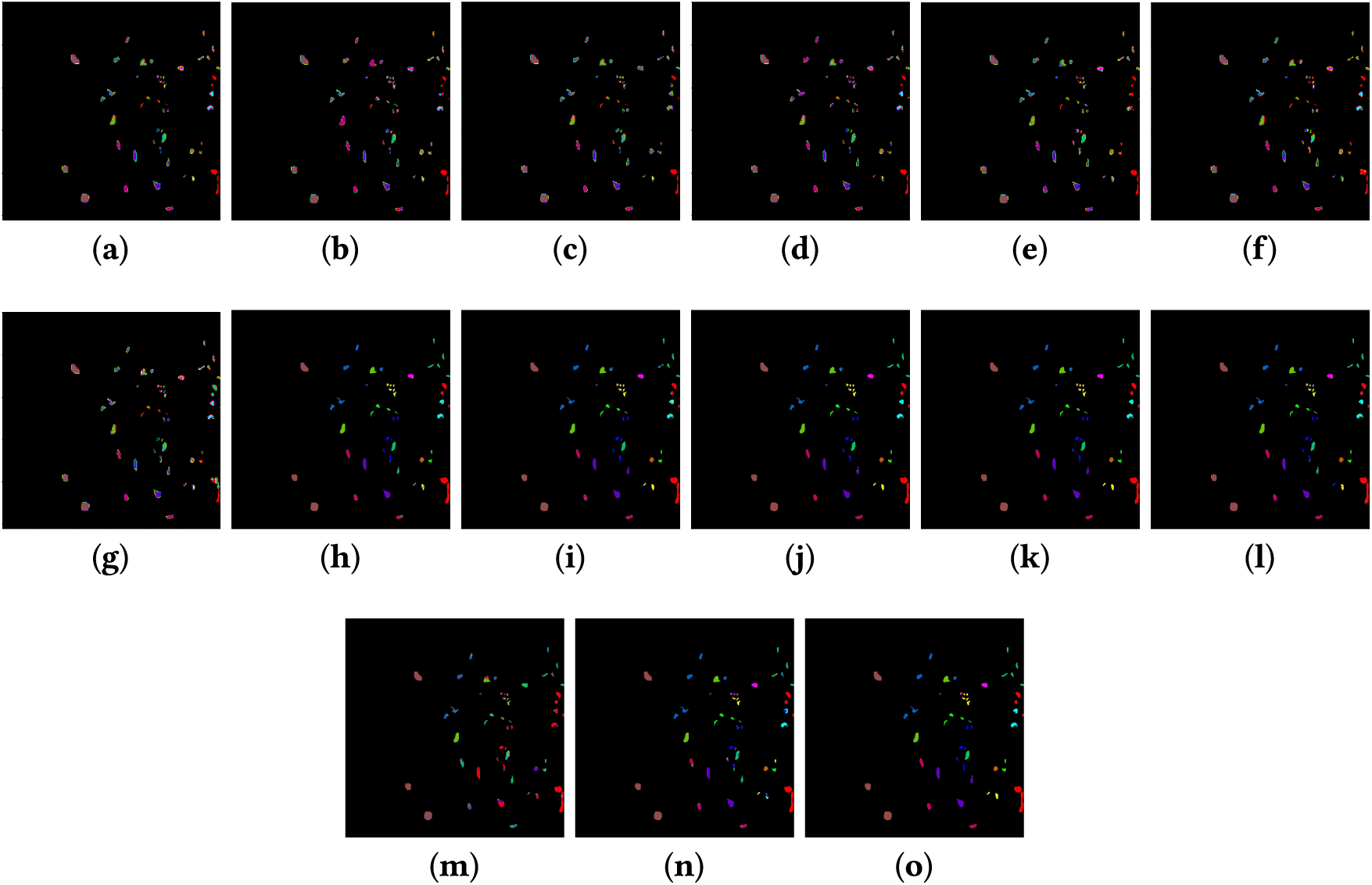
Figure 11: Classification maps generated by different methods on the KSC dataset are displayed sequentially. (From Left to Right) (a) ground truth, (b) SVM-RBF, (c) CCF-200, (d) 2-D CNN [37], (e) GCNN [33], (f) FADCNN [40], (g) NL-GCNN [32], (h) ViT [54], (i) WaveFormer [60], (j) PMCN [59], (k) PyFormer [55], (l) SwinT [56], (m) MorpMamba [82], (n) DiMA [83], and (o) (Proposed Approach) FEAM-Swin.

Across all four benchmark datasets SA, IP, PU, and KSC, comparative analysis reveals a clear hierarchy in classification performance. While conventional and early CNN-based approaches establish a reasonable performance baseline, contemporary Transformer-based architectures achieve substantially higher classification accuracy. Within this landscape, the proposed FEAM-Swin consistently achieves the highest OA, AA, and κ scores across every evaluated dataset, demonstrating its superior classification capability relative to all competing approaches. The superior performance of FEAM-Swin can be attributed to the synergistic interaction of two complementary mechanisms: (1) the FEAM module, which performs frequency-aware channel recalibration of input feature maps prior to attention computation, and (2) the Dynamic Context Scaling (DCS) mechanism, which enriches the window-based self-attention by scaling attention weights with global contextual information derived from the attention matrix itself. Together, these mechanisms enable FEAM-Swin to capture both local high-frequency spectral variations and global contextual dependencies with minimal computational overhead.

3.4 Ablation Analysis

3.4.1 Analysis of Number of Attention

Fig. 12 presents the validation accuracy of the proposed FEAM-Swin model across four hyperspectral benchmark datasets KSC, PU, IP, and SA under different attention head configurations (2, 4, and 8 heads). The resulting performance trends show meaningful insights into how well the model captures spectral dependencies and adapts to the varying levels of complexity inherent in each dataset.

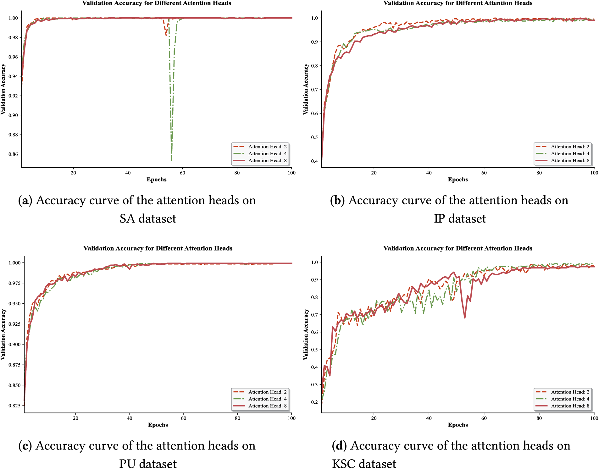
Figure 12: Illustrates the effect of varying the number of attention heads within the proposed FEAM-Swin architecture.

On the KSC dataset, validation accuracy demonstrates a consistent upward trajectory over 100 training epochs, starting from approximately 0.2 and progressively approaching 1.0. All three attention head configurations (2, 4, and 8) exhibit considerable fluctuation during the early and mid-training stages, with the 4-head configuration experiencing a notable accuracy drop around epoch 55. Toward the later epochs, the 2-head and 4-head configurations converge slightly closer to 1.0, while the 8-head configuration stabilizes at a marginally lower plateau, suggesting that moderate attention head counts may offer a better balance between representational capacity and training stability on this dataset.

The validation accuracy results for the PU dataset further reinforce the robustness of the FEAM-Swin model. As depicted in Fig. 12, accuracy values remain consistently high throughout training, spanning a range between 0.825 and 1.0 across all 100 epochs. The stability observed across all three attention head configurations (2, 4, and 8) reflects the model’s strong capacity for generalisation on this dataset. While all configurations converge to near-perfect accuracy, the 8-head setup achieves a slight edge over the 2 and 4-head variants, converging more smoothly and maintaining a marginally higher validation accuracy in the early epochs. This advantage indicates that a greater number of attention heads enables more effective learning of spectral correlations, allowing the model to capture richer feature representations within the PU dataset.

For the IP dataset, validation accuracy begins at approximately 0.4 in the earliest epochs and steadily climbs toward 1.0 over the course of 100 training epochs, reflecting a more demanding learning process relative to other datasets. In the initial stages of training, the 2-head and 4-head configurations converge slightly faster than the 8-head variant, though all three configurations ultimately reach comparable near-perfect accuracy by the later epochs. The moderate fluctuations observed during mid-training are indicative of the greater spectral complexity inherent in the IP dataset. Nevertheless, FEAM-Swin demonstrates strong adaptability across all attention head settings, consistently progressing toward high validation accuracy and confirming its effectiveness in extracting discriminative spectral features for HSI classification.

On the SA dataset, all three attention head configurations exhibit remarkably rapid convergence, with validation accuracy rising sharply from approximately 0.86–0.94 in the earliest epochs to near-perfect scores of 1.0 within the first 10 epochs. The 8-head configuration demonstrates the most stable training trajectory, maintaining a consistent accuracy of 1.0 throughout the entire training process without any notable fluctuations. In contrast, both the 2-head and 4-head configurations experience sudden accuracy drops around epoch 55, with the 4-head variant suffering a particularly severe decline, falling to approximately 0.85 before recovering back to 1.0 in subsequent epochs. Despite these transient instabilities, all configurations ultimately converge to near-perfect validation accuracy by the end of training. The superior stability of the 8-head configuration on the SA dataset further underscores the benefit of increased attention capacity in capturing the relatively well-separated spectral features characteristic of this dataset.

A closer examination of the validation accuracy curves across all four datasets indicates subtle trends that go beyond a simple relationship between attention head count and performance. On the SA dataset, the 8-head configuration demonstrates the most stable convergence, maintaining near-perfect accuracy throughout training, while the 2-head and 4-head variants experience transient but sharp drops around epoch 55 before recovering. On the IP dataset, the 2-head and 4-head configurations initially converge faster than the 8-head variant, though all three ultimately reach comparable accuracy levels by the final epochs. On the PU dataset, all three configurations converge smoothly to near-perfect accuracy with minimal fluctuation, with the 8-head configuration showing a marginal edge in early-epoch stability. For the KSC dataset, all configurations exhibit considerable fluctuation during mid-training, with the 4-head variant suffering a notable dip around epoch 55, and the 2-head and 4-head setups ultimately converging marginally closer to 1.0 than the 8-head configuration.

The varying accuracy trajectories across four datasets reflect their differing levels of spectral complexity. The KSC and IP datasets exhibit wider accuracy ranges and greater mid-training instability, indicating that they demand more extensive learning to achieve high performance. The SA and PU datasets, in contrast, reach near-perfect accuracy more rapidly and finish training with the highest overall accuracy; PU exhibit minimal fluctuation throughout, while SA shows fast initial convergence but a transient, sharp instability around epoch 55 for the 2- and 4-head configurations before recovering to near-perfect accuracy.

The validation accuracy results across all four datasets affirm the adaptability and robustness of the proposed FEAM-Swin model for HSI classification. Rather than uniformly favouring the highest attention head count, the results suggest that optimal configuration may vary depending on dataset characteristics, with the model consistently demonstrating strong convergence and high final accuracy regardless of the attention head setting employed.

3.4.2 Analysis of Patch Size Variations

In HSI classification, patch size selection is a critical design choice that directly influences how well a model captures spatial and spectral information. As illustrated in Fig. 13, FEAM-Swin was evaluated under five different patch size settings (2 × 2, 4 × 4, 6 × 6, 10 × 10, and 12 × 12) across all four benchmark datasets, revealing distinct sensitivity patterns for each.

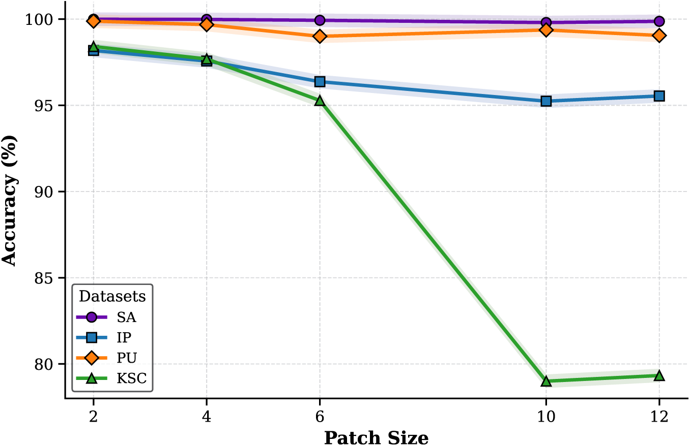
Figure 13: Impact of different patch sizes (2 × 2, 4 × 4, 6 × 6, 10 × 10, and 12 × 12) on the classification performance of the proposed FEAM-Swin model.

The SA dataset shows low sensitivity to patch size variation, with classification accuracy remaining near-perfect across all configurations (99.97%, 99.98%, 99.93%, 99.80%, 99.87% at patch sizes 2, 4, 6, 10, and 12, respectively). Accuracy peaks at a patch size of 4 (99.98%) and dips slightly at patch size 10 (99.80%), confirming that FEAM-Swin reliably extracts discriminative spectral features from this dataset across a wide range of spatial context sizes.

On the IP dataset, a more variable trend is observed. Performance peaks at a patch size of 2, 98.83%, declines gradually through patch sizes 4, 98.17% and 6, 98.10%, dips further at patch size 10, 97.95%, and partially recovers at patch size 12, 98.68%. This non-monotonic pattern suggests that intermediate patch sizes may inadvertently introduce spatial noise or dilute spectrally relevant features for this dataset.

The PU dataset shows moderate sensitivity to patch size, with accuracy ranging from 99.00% to 99.87% across the five configurations tested (99.87%, 99.68%, 99.00%, 99.37%, and 99.05% at patch sizes 2, 4, 6, 10, and 12, respectively). The peak accuracy of 99.87% is attained at the smallest patch size of 2, while the lowest value of 99.00% occurs at a patch size of 6, after which accuracy partially recovers at larger patch sizes.

The KSC dataset presents the most pronounced sensitivity to patch size, as clearly visible in the sharp downward trajectory of the green curve in Fig. 13. While a patch size of 2 yields the highest accuracy of 98.16%, performance deteriorates substantially as patch size grows, dropping to 95.11% at patch size 4, 89.46% at patch size 6, and reaching its lowest values of 79.35% and 79.40% at patch sizes 10 and 12, respectively. This steep decline highlights the importance of preserving fine-grained spatial detail for the KSC dataset, where larger patch sizes appear to obscure the subtle spatial structures that are critical for accurate classification.

These findings underscore the necessity of dataset-specific patch size tuning when deploying FEAM-Swin. Datasets with complex spatial structures, such as KSC, benefit significantly from smaller patch sizes, while datasets with more uniform spectral characteristics, such as SA and PU, remain robust across a broader range of configurations.

3.4.3 Effect of Training Sample Ratio

To evaluate the robustness of the proposed FEAM-Swin framework under different levels of labeled training data, an ablation study was conducted by varying the proportion of training samples from 1%, 2%, 10%, 20%, and 30% while keeping all other experimental settings unchanged. The obtained overall accuracies (OA) on the four benchmark hyperspectral datasets are summarized in Table 11.

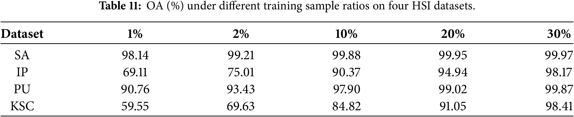
The results demonstrate that the proposed model consistently achieves improved classification performance as the number of labeled training samples increases. Specifically, on the SA dataset, the proposed method already achieves an OA of 98.14% using only 1% of the training samples, which further improves to 99.97% with 30% of the training data. This indicates that the proposed feature extraction strategy can effectively capture highly discriminative spectral-spatial representations even under extremely limited supervision.

A similar trend is observed on the more challenging IP dataset. Due to the higher spectral similarity among land-cover classes and the relatively limited number of samples, the OA starts from 69.11% at 1% training data and progressively increases to 98.17% when 30% of the labeled samples are used. The substantial improvement of nearly 29 percentage points demonstrates the excellent scalability of the proposed architecture with increasing training information.

For the PU dataset, the proposed model achieves 90.76% OA using only 1% of the training samples and rapidly reaches 99.87% with 30% training data. The relatively small performance gap compared with the other datasets indicates that the urban scene provides sufficiently discriminative spectral-spatial information, allowing the proposed FEAM-Swin architecture to learn effective representations even with very limited annotations.

The KSC dataset is the most challenging among the four datasets because of its high spectral complexity and limited labeled samples. Nevertheless, the proposed method steadily improves from 59.55% OA at 1% training data to 98.41% OA at 30%, representing the largest relative improvement among all datasets. This observation confirms that the proposed frequency-enhanced attention mechanism effectively exploits both local and global spectral dependencies as additional labeled samples become available.

The experimental results indicate that the proposed FEAM-Swin model exhibits excellent robustness across different training sample ratios. Even with extremely limited labeled data, the framework maintains competitive classification accuracy, while additional training samples consistently lead to further performance improvements. These findings demonstrate the strong generalization capability and data efficiency of the proposed architecture, making it suitable for practical HSI classification scenarios where labeled samples are often scarce.

3.4.4 Component-Wise Ablation Analysis

To systematically quantify the contribution of each architectural component of FEAM-Swin, we conducted a comprehensive ablation study by progressively adding components to a baseline Swin Transformer. Eight configurations were evaluated on all four benchmark datasets as summarized in Table 12.

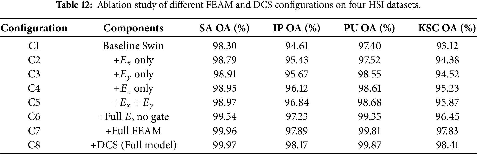
The configurations were defined as follows. C1 represents the baseline Swin Transformer without FEAM. C2 and C3 extend C1 with only the spatial height gradient (Ex) and spatial width gradient (Ey), respectively, whereas C4 incorporates only the spectral gradient (Ez). C5 combines the two spatial gradients (Ex+Ey) without the spectral component. C6 employs the full gradient descriptor (Ex+Ey+Ez) but excludes the gating network, while C7 incorporates the complete FEAM module, including all three gradient components and the gating network. Finally, C8 represents the complete FEAM-Swin architecture, which augments C7 with Dynamic Context Scaling.

The results reveal several important insights. First, comparing C1 and C8 directly establishes that the proposed FEAM module provides consistent and substantial performance improvements across all four datasets, confirming that frequency-aware channel recalibration is the primary driver of FEAM-Swin’s superior performance. Second, comparing C2, C3, and C4 individually demonstrates that all three gradient directions contribute positively, with the spectral gradient (Ez) providing the most distinctive improvement on spectrally complex datasets such as KSC and IP. Third, comparing C5 and C6 with C7 confirms that both the spectral gradient component and the learnable gating network are essential for achieving optimal performance, as removing either degrades results across all datasets. Finally, comparing C7 and C8 quantifies the additional contribution of the Dynamic Context Scaling mechanism, which provides further consistent improvements by enriching the attention modulation with global contextual scaling.

3.4.5 Inference Efficiency Analysis

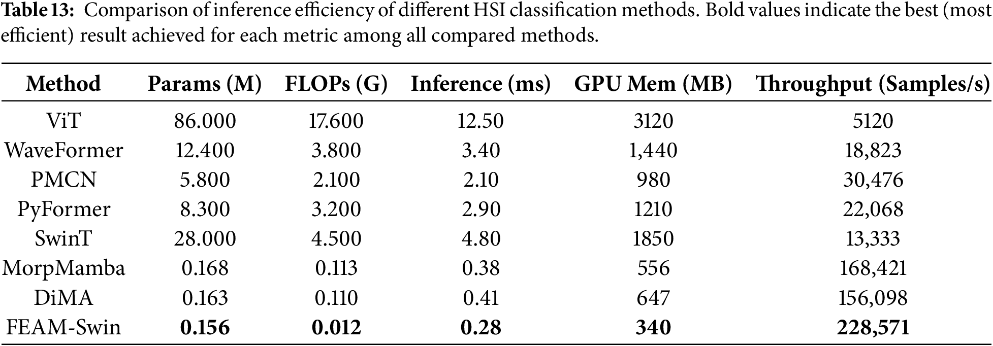
In addition to classification accuracy, practical deployment requires models with high inference efficiency and low computational overhead. Therefore, we compare the proposed FEAM-Swin with several representative HSI classification methods in terms of the number of parameters, floating-point operations (FLOPs), inference latency, GPU memory consumption, and throughput. As shown in Table 13, FEAM-Swin achieves the highest inference efficiency while maintaining superior classification performance. Specifically, it requires only 0.156M parameters and 0.012G FLOPs, which are substantially lower than those of existing transformer-based methods. Furthermore, FEAM-Swin attains an inference time of 0.28 ms, consumes only 340 MB of GPU memory, and achieves a throughput of 228,571 samples/s, demonstrating its suitability for real-time and resource-constrained HSI classification applications. These results indicate that the proposed feature enhancement strategy introduces only a negligible computational overhead while providing significant improvements in classification accuracy. Moreover, the excellent trade-off between predictive performance and computational efficiency makes FEAM-Swin highly suitable for deployment in practical remote sensing systems, including edge devices and real-time hyperspectral image analysis platforms.

3.4.6 Computational Complexity Analysis

Training efficiency is a key practical consideration when assessing the viability of deep learning architectures for real-world deployment. To evaluate the computational cost of the proposed FEAM-Swin, its training time was benchmarked against competitive Transformer-based methods DiMA, SwinT, PyFormer, PMCN, WaveFormer, ViT and MorpMamba across the SA, IP, PU, and KSC datasets. All models were trained on identical hardware, with method-specific optimization settings, to ensure a fair comparison. As depicted in Fig. 14, FEAM-Swin achieves the shortest training time across every dataset by a considerable margin.

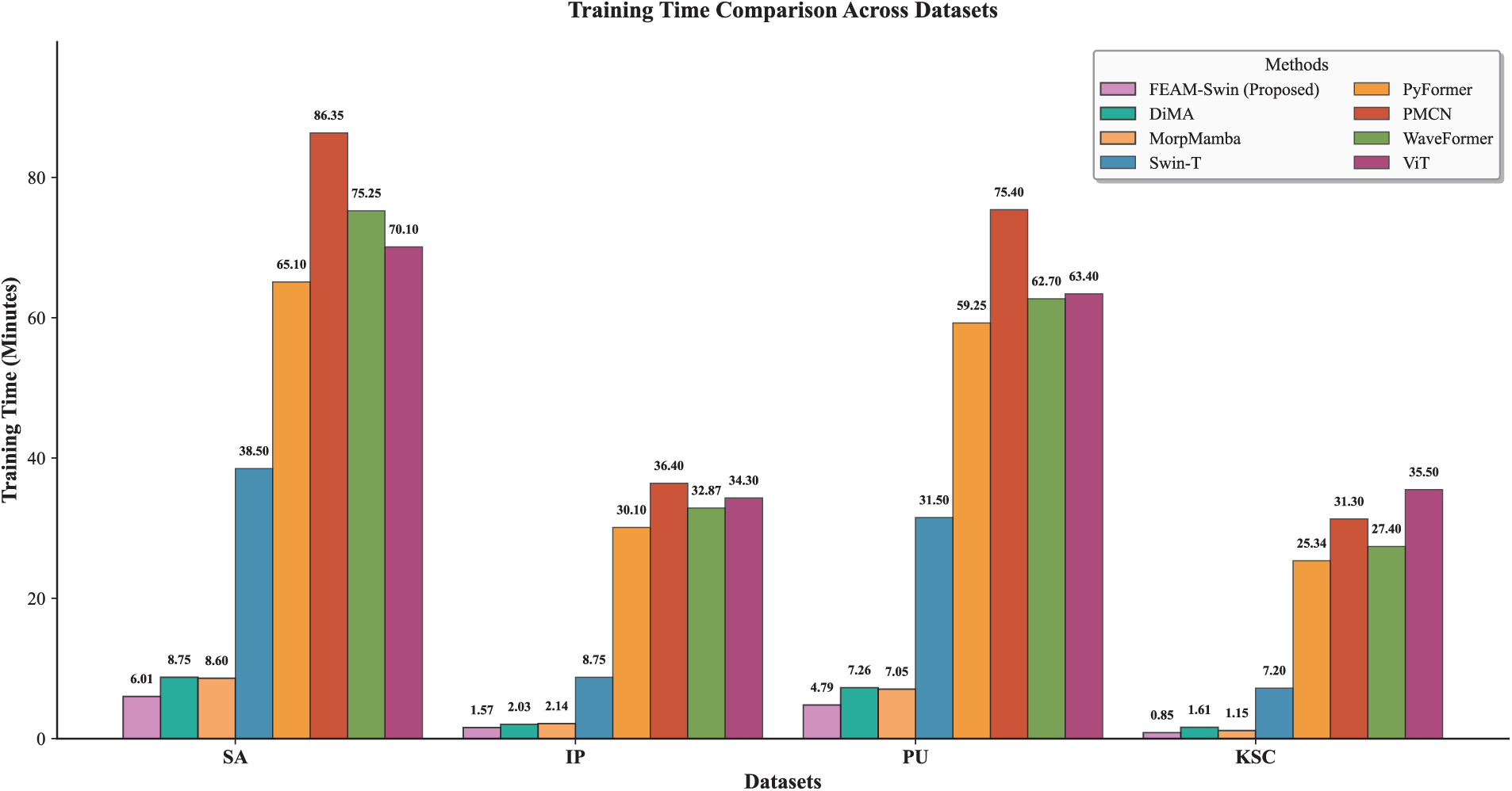
Figure 14: Computation complexity: total time taken (minutes) for training of the proposed FEAM-Swin model against the comparative methods.

On the SA dataset, FEAM-Swin completes training in just 6.01 min, compared to 8.75 min for DiMA, 8.60 min for MorpMamba, 38.50 min for SwinT, 65.10 min for PyFormer, 86.35 min for PMCN, 75.25 min for WaveFormer, and 70.10 min for ViT. The efficiency advantage is even more striking on the IP dataset, where FEAM-Swin requires only 1.57 min, while competing methods range from 2.03 min (DiMA) to 36.40 min (PMCN). On the PU dataset, FEAM-Swin’s training time of 4.79 min stands in sharp contrast to DiMA (7.26 min), MorpMamba (7.05 min), PyFormer (59.25 min) and PMCN (75.40 min), representing reductions ranging from roughly 32%–34% (MorpMamba, DiMA) to over 90% (PyFormer, PMCN). The KSC dataset further reinforces this pattern, with FEAM-Swin completing training in just 0.85 min nearly nine times faster than SwinT (7.20 min) and more than forty times faster than ViT (35.50 min).

These results collectively demonstrate that FEAM-Swin delivers not only superior classification performance but also exceptional computational efficiency. The dramatic reductions in training time across all datasets can be attributed to the model’s streamlined attention mechanisms and dynamic spectral feature aggregation strategy, which minimize computational overhead without sacrificing representational capacity. These characteristics make FEAM-Swin a highly practical and scalable solution for large-scale HSI classification applications.

4  Conclusion and Future Work

In this paper, we presented FEAM-Swin, a lightweight frequency-aware Swin Transformer framework designed for efficient and accurate HSI classification. The proposed architecture introduces a novel Frequency-Enhanced Attention Modulator (FEAM) that captures local spectral–spatial frequency variations through gradient-based energy estimation, enabling adaptive channel recalibration without relying on computationally expensive explicit frequency transforms such as Fourier or wavelet decompositions. By seamlessly embedding FEAM within hierarchical Swin Transformer blocks, the proposed model enhances discriminative feature learning while preserving the computational efficiency of window-based self-attention. Extensive experiments conducted on four widely adopted benchmark hyperspectral datasets SA, IP, PU, and KSC validate the effectiveness and generalizability of the proposed framework. FEAM-Swin consistently outperforms competing CNN and state-of-the-art Transformer-based approaches across all four benchmark datasets. Furthermore, the computational complexity analysis demonstrates that FEAM-Swin achieves the lowest training times across all evaluated datasets by a substantial margin, confirming its practical viability for real-world deployment under resource-constrained conditions.

Despite these promising results, several areas remain open for future investigation. Although the window-based attention mechanism in FEAM-Swin effectively models local and semi-global dependencies, it may still impose limitations on global receptive field coverage in highly complex and heterogeneous scenes. Future work will explore the integration of cross-attention modules and dynamic multi-scale attention strategies to further broaden contextual modeling capacity. Additionally, extending FEAM-Swin to semi-supervised and few-shot learning settings represents a compelling direction, as the scarcity of labeled training samples remains a persistent challenge in remote sensing. Incorporating temporal–spectral modeling to support time-series hyperspectral analysis is another promising area, enabling the framework to handle dynamic land-cover changes over time. We will also extend the evaluation of FEAM-Swin to include: (1) cross-dataset transfer learning experiments evaluating the transferability of frequency-aware features learned on one dataset to unseen target datasets; (2) robustness analysis under realistic degradation conditions including missing spectral bands, atmospheric noise, and spectral distortions; and (3) evaluation on additional benchmark datasets beyond the four considered in this study, such as Houston 2013, Houston 2018, and Trento, to comprehensively assess generalizability across diverse geographical regions and sensor characteristics. These directions aim to further enhance the generalization capability, scalability, and real-world applicability of the proposed FEAM-Swin framework.

Acknowledgement: This work was supported by the 2023 Excellent Science and Technology Innovation Team of Jiangsu Province Universities (Real-time Industrial Internet of Things). The authors would also like to thank the Princess Nourah bint Abdulrahman University Researchers Supporting Project number (PNURSP2026R896), Princess Nourah bint Abdulrahman University, Riyadh, Saudi Arabia.

Funding Statement: This work was funded by the 2023 Excellent Science and Technology Innovation Team of Jiangsu Province Universities (Real-time Industrial Internet of Things), and the Princess Nourah bint Abdulrahman University Researchers Supporting Project number (PNURSP2026R896), Princess Nourah bint Abdulrahman University, Riyadh, Saudi Arabia.

Author Contributions: The authors confirm contribution to the paper as follows: Conceptualization, Farhan Ullah and Irfan Ullah; methodology, Farhan Ullah, Irfan Ullah and Khalil Khan; software, Farhan Ullah; validation, Farhan Ullah, Irfan Ullah, Khalil Khan, Sarra Ayouni and Quan Wang; formal analysis, Farhan Ullah and Irfan Ullah; investigation, Farhan Ullah and Khalil Khan; resources, Sarra Ayouni and Quan Wang; data curation, Farhan Ullah and Irfan Ullah; writing—original draft preparation, Farhan Ullah; writing—review and editing, Irfan Ullah, Khalil Khan, Sarra Ayouni and Quan Wang; visualization, Farhan Ullah; supervision, Sarra Ayouni and Quan Wang; project administration, Quan Wang; funding acquisition, Sarra Ayouni and Quan Wang. All authors reviewed and approved the final version of the manuscript.

Availability of Data and Materials: This study uses publicly available benchmark hyperspectral remote sensing datasets (Indian Pines, Salinas, University of Pavia, and Kennedy Space Center), permanently archived on IEEE DataPort under https://dx.doi.org/10.21227/mpp2-my34, originally curated by the Grupo de Inteligencia Computacional (GIC), University of the Basque Country (UPV/EHU) and also accessible at https://www.ehu.eus/ccwintco/index.php/Hyperspectral_Remote_Sensing_Scenes (accessed on 1 June 2026).

Ethics Approval: Not applicable.

Conflicts of Interest: The authors declare no conflicts of interest.

References

1. Huang S, Zhang H, Pižurica A. Subspace clustering for hyperspectral images via dictionary learning with adaptive regularization. IEEE Trans Geosci Remote Sens. 2022;60(34):5524017. doi:10.1109/tgrs.2021.3127536. [Google Scholar] [CrossRef]

2. Wang L, Zuo B, Le Y, Chen Y, Li J. Penetrating remote sensing: next-generation remote sensing for transparent earth. Innovation. 2023;4(6):100519. doi:10.1016/j.xinn.2023.100519. [Google Scholar] [CrossRef]

3. Peyghambari S, Zhang Y. Hyperspectral remote sensing in lithological mapping, mineral exploration, and environmental geology: an updated review. J Appl Remote Sens. 2021;15(03):31501. doi:10.1117/1.jrs.15.031501. [Google Scholar] [CrossRef]

4. Stuart MB, McGonigle AJS, Willmott JR. Hyperspectral imaging in environmental monitoring: a review of recent developments and technological advances in compact field deployable systems. Sensors. 2019;19(14):3071. [Google Scholar]

5. Lv M, Li W, Tao R, Lovell NH, Yang Y, Tu T, et al. Spatial-spectral density peaks-based discriminant analysis for membranous nephropathy classification using microscopic hyperspectral images. IEEE J Biomed Health Inform. 2021;25(8):3041–51. doi:10.1109/jbhi.2021.3050483. [Google Scholar] [PubMed] [CrossRef]

6. Blanzieri E, Melgani F. Nearest neighbor classification of remote sensing images with the maximal margin principle. IEEE Trans Geosci Remote Sens. 2008;46(6):1804–11. doi:10.1109/tgrs.2008.916090. [Google Scholar] [CrossRef]

7. Melgani F, Bruzzone L. Classification of hyperspectral remote sensing images with support vector machines. IEEE Trans Geosci Remote Sens. 2004;42(8):1778–90. doi:10.1109/tgrs.2004.831865. [Google Scholar] [CrossRef]

8. Zhang Y, Cao G, Li X, Wang B. Cascaded random forest for hyperspectral image classification. IEEE J Sel Top Appl Earth Obs Remote Sens. 2018;11(4):1082–94. doi:10.1109/jstars.2018.2809781. [Google Scholar] [CrossRef]

9. Chen Y, Nasrabadi NM, Tran TD. Classification for hyperspectral imagery based on sparse representation. In: Proceedings of the 2010 2nd Workshop on Hyperspectral Image and Signal Processing: Evolution in Remote Sensing; 2010 Jun 14–16; Reykjavik, Iceland. p. 1–4. [Google Scholar]

10. Peng J, Li L, Tang YY. Maximum likelihood estimation-based joint sparse representation for the classification of hyperspectral remote sensing images. IEEE Trans Neural Netw Learn Syst. 2019;30(6):1790–802. doi:10.1109/tnnls.2018.2874432. [Google Scholar] [CrossRef]

11. Xia J, Falco N, Benediktsson JA, Du P, Chanussot J. Hyperspectral image classification with rotation random forest via KPCA. IEEE J Sel Top Appl Earth Obs Remote Sens. 2017;10(4):1601–9. doi:10.1109/jstars.2016.2636877. [Google Scholar] [CrossRef]

12. Li W, Prasad S, Fowler JE, Bruce LM. Locality-preserving discriminant analysis in kernel-induced feature spaces for hyperspectral image classification. IEEE Geosci Remote Sens Lett. 2011;8(5):894–8. doi:10.1109/lgrs.2011.2128854. [Google Scholar] [CrossRef]

13. Zhang X, Gao Z, Jiao L, Zhou H. Multifeature hyperspectral image classification with local and nonlocal spatial information via Markov random field in semantic space. IEEE Trans Geosci Remote Sens. 2018;56(3):1409–24. doi:10.1109/tgrs.2017.2762593. [Google Scholar] [CrossRef]

14. Ren Y, Liao L, Maybank SJ, Zhang Y, Liu X. Hyperspectral image spectral-spatial feature extraction via tensor principal component analysis. IEEE Geosci Remote Sens Lett. 2017;14(9):1431–5. doi:10.1109/lgrs.2017.2686878. [Google Scholar] [PubMed] [CrossRef]

15. Peng J, Sun W, Du Q. Self-paced joint sparse representation for the classification of hyperspectral images. IEEE Trans Geosci Remote Sens. 2019;57(2):1183–94. doi:10.1109/tgrs.2018.2865102. [Google Scholar] [CrossRef]

16. Huang S, Zhang H, Xue J, Pizurica A. Heterogeneous regularization-based tensor subspace clustering for hyperspectral band selection. IEEE Trans Neural Netw Learn Syst. 2023;34(11):9259–73. doi:10.1109/tnnls.2022.3157711. [Google Scholar] [PubMed] [CrossRef]

17. Huang S, Zhang H, Pizurica A. A structural subspace clustering approach for hyperspectral band selection. IEEE Trans Geosci Remote Sens. 2022;60:5509515. doi:10.1109/tgrs.2021.3102422. [Google Scholar] [CrossRef]

18. Camps-Valls G, Gomez-Chova L, Muñoz-Marí J, Vila-Francés J, Calpe-Maravilla J. Composite kernels for hyperspectral image classification. IEEE Geosci Remote Sens Lett. 2006;3(1):93–7. doi:10.1109/lgrs.2005.857031. [Google Scholar] [CrossRef]

19. Sadeghi-Tehran P, Virlet N, Hawkesford MJ. A neural network method for classification of sunlit and shaded components of wheat canopies in the field using high-resolution hyperspectral imagery. Remote Sens. 2021;13(5):898. doi:10.3390/rs13050898. [Google Scholar] [CrossRef]

20. Jia S, Deng B, Zhu J, Jia X, Li Q. Local binary pattern-based hyperspectral image classification with superpixel guidance. IEEE Trans Geosci Remote Sens. 2018;56(2):749–59. doi:10.1109/tgrs.2017.2754511. [Google Scholar] [CrossRef]

21. Liu J, Wu Z, Li J, Plaza A, Yuan Y. Probabilistic-kernel collaborative representation for spatial–spectral hyperspectral image classification. IEEE Trans Geosci Remote Sens. 2016;54(4):2371–84. doi:10.1109/tgrs.2015.2500680. [Google Scholar] [CrossRef]

22. Fauvel M, Chanussot J, Benediktsson JA. Kernel principal component analysis for the classification of hyperspectral remote sensing data over urban areas. EURASIP J Adv Signal Process. 2009;2009(1):783194. doi:10.1155/2009/783194. [Google Scholar] [CrossRef]

23. Fauvel M, Benediktsson JA, Chanussot J, Sveinsson JR. Spectral and spatial classification of hyperspectral data using SVMs and morphological profiles. IEEE Trans Geosci Remote Sens. 2008;46(11):3804–14. doi:10.1109/tgrs.2008.922034. [Google Scholar] [CrossRef]

24. Zhao C, Zhu W, Feng S. Superpixel guided deformable convolution network for hyperspectral image classification. IEEE Trans Image Process. 2022;31:3838–51. [Google Scholar]

25. Liu R, Luo T, Huang S, Wu Y, Jiang Z, Zhang H. CrossMatch: cross-view matching for semi-supervised remote sensing image segmentation. IEEE Trans Geosci Remote Sens. 2024;62:5650515. doi:10.1109/tgrs.2024.3507050. [Google Scholar] [CrossRef]

26. Ullah F, Zhang B, Khan RU, Chung TS, Attique M, Khan K, et al. Deep Edu: a deep neural collaborative filtering for educational services recommendation. IEEE Access. 2020;8:110915–28. [Google Scholar]

27. Ullah F, Zhang B, Zou G, Ullah I, Qamar AM, Durr-e-Nayab, et al. Large-scale distributive matrix collaborative filtering for recommender system. In: Proceedings of the 2020 International Conference on Computing, Networks and Internet of Things; 2020 Apr 24–26; Sanya, China. p. 55–9. [Google Scholar]

28. Ullah F, Zhang B, Khan RU, Ullah I, Khan A, Qamar AM. Visual-based items recommendation using deep neural network. In: Proceedings of the 2020 International Conference on Computing, Networks and Internet of Things; 2020 Apr 24–26; Sanya, China. New York, NY, USA: Association for Computing Machinery; 2020. p. 122–6. doi:10.1145/3398329.3398359. [Google Scholar] [CrossRef]

29. Liang L, Zhang S, Li J. Multiscale DenseNet meets with bi-RNN for hyperspectral image classification. IEEE J Sel Top Appl Earth Obs Remote Sens. 2022;15:5401–15. doi:10.1109/jstars.2022.3187009. [Google Scholar] [PubMed] [CrossRef]

30. Zhang F, Bai J, Zhang J, Xiao Z, Pei C. An optimized training method for GAN-based hyperspectral image classification. IEEE Geosci Remote Sens Lett. 2021;18(10):1791–5. doi:10.1109/lgrs.2020.3009017. [Google Scholar] [CrossRef]

31. Liu Q, Xiao L, Yang J, Wei Z. CNN-enhanced graph convolutional network with pixel- and superpixel-level feature fusion for hyperspectral image classification. IEEE Trans Geosci Remote Sens. 2021;59(10):8657–71. doi:10.1109/tgrs.2020.3037361. [Google Scholar] [PubMed] [CrossRef]

32. Mou L, Lu X, Li X, Zhu XX. Nonlocal graph convolutional networks for hyperspectral image classification. IEEE Trans Geosci Remote Sens. 2020;58(12):8246–57. doi:10.1109/tgrs.2020.2973363. [Google Scholar] [CrossRef]

33. Hong D, Gao L, Yao J, Zhang B, Plaza A, Chanussot J. Graph convolutional networks for hyperspectral image classification. IEEE Trans Geosci Remote Sens. 2021;59(7):5966–78. doi:10.1109/tgrs.2020.3015157. [Google Scholar] [CrossRef]

34. Ullah F, Long Y, Ullah I, Khan RU, Khan S, Khan K, et al. Deep hyperspectral shots: deep snap smooth wavelet convolutional neural network shots ensemble for hyperspectral image classification. IEEE J Sel Top Appl Earth Obs Remote Sens. 2024;17:14–34. doi:10.1109/jstars.2023.3314900. [Google Scholar] [CrossRef]

35. Hu W, Huang Y, Wei L, Zhang F, Li H. Deep convolutional neural networks for hyperspectral image classification. J Sens. 2015;2015(1):258619. [Google Scholar]

36. Makantasis K, Karantzalos K, Doulamis A, Doulamis N. Deep supervised learning for hyperspectral data classification through convolutional neural networks. In: Proceedings of the 2015 IEEE International Geoscience and Remote Sensing Symposium (IGARSS); 2015 Jul 26–31; Milan, Italy. p. 4959–62. [Google Scholar]

37. Ge Z, Cao G, Li X, Fu P. Hyperspectral image classification method based on 2D–3D CNN and multibranch feature fusion. IEEE J Sel Top Appl Earth Obs Remote Sens. 2020;13:5776–88. doi:10.1109/jstars.2020.3024841. [Google Scholar] [CrossRef]

38. Chen Y, Jiang H, Li C, Jia X, Ghamisi P. Deep feature extraction and classification of hyperspectral images based on convolutional neural networks. IEEE Trans Geosci Remote Sens. 2016;54(10):6232–51. doi:10.1109/tgrs.2016.2584107. [Google Scholar] [CrossRef]

39. Roy SK, Krishna G, Dubey SR, Chaudhuri BB. HybridSN: exploring 3-D–2-D CNN feature hierarchy for hyperspectral image classification. IEEE Geosci Remote Sens Lett. 2020;17(2):277–81. doi:10.1109/lgrs.2019.2918719. [Google Scholar] [CrossRef]

40. Yu C, Han R, Song M, Liu C, Chang CI. Feedback attention-based dense CNN for hyperspectral image classification. IEEE Trans Geosci Remote Sens. 2022;60:5501916. doi:10.1109/tgrs.2021.3058549. [Google Scholar] [PubMed] [CrossRef]

41. Zhong Z, Li J, Luo Z, Chapman M. Spectral–spatial residual network for hyperspectral image classification: a 3-D deep learning framework. IEEE Trans Geosci Remote Sens. 2018;56(2):847–58. [Google Scholar]

42. Zhang C, Li G, Du S. Multi-scale dense networks for hyperspectral remote sensing image classification. IEEE Trans Geosci Remote Sens. 2019;57(11):9201–22. doi:10.1109/tgrs.2019.2925615. [Google Scholar] [CrossRef]

43. Dong S, Feng W, Quan Y, Dauphin G, Gao L, Xing M. Deep ensemble CNN method based on sample expansion for hyperspectral image classification. IEEE Trans Geosci Remote Sens. 2022;60:5531815. [Google Scholar]

44. Sun H, Zheng X, Lu X, Wu S. Spectral–spatial attention network for hyperspectral image classification. IEEE Trans Geosci Remote Sens. 2020;58(5):3232–45. doi:10.1109/tgrs.2020.2994057. [Google Scholar] [CrossRef]

45. Lu Z, Xu B, Sun L, Zhan T, Tang S. 3-D channel and spatial attention based multiscale spatial–spectral residual network for hyperspectral image classification. IEEE J Sel Top Appl Earth Obs Remote Sens. 2020;13:4311–24. [Google Scholar]

46. Woo S, Park J, Lee JY, Kweon IS. CBAM: convolutional block attention module. In: Proceedings of the European Conference on Computer Vision (ECCV); 2018 Sep 8–14; Munich, Germany. p. 3–19. [Google Scholar]

47. Zhu M, Jiao L, Liu F, Yang S, Wang J. Residual spectral–spatial attention network for hyperspectral image classification. IEEE Trans Geosci Remote Sens. 2021;59(1):449–62. doi:10.1109/tgrs.2020.2994057. [Google Scholar] [CrossRef]

48. Dosovitskiy A, Beyer L, Kolesnikov A, Weissenborn D, Zhai X, Unterthiner T, et al. An image is worth 16×16 words: transformers for image recognition at scale. arXiv:2010.11929. 2020. [Google Scholar]

49. Vaswani A, Shazeer N, Parmar N, Uszkoreit J, Jones L, Gomez AN, et al. Attention is all you need. In: Proceedings of the 31st International Conference on Neural Information Processing Systems; 2017 Dec 4–9; Long Beach, CA, USA. p. 6000–10. [Google Scholar]

50. Xie E, Chen N, Peng J, Sun W, Du Q, You X. Semantic and spatial-spectral feature fusion transformer network for the classification of hyperspectral image. CAAI Trans Intell Technol. 2023;8(4):1308–22. doi:10.1049/cit2.12201. [Google Scholar] [CrossRef]

51. Zhao F, Li S, Zhang J, Liu H. Convolution transformer fusion splicing network for hyperspectral image classification. IEEE Geosci Remote Sens Lett. 2023;20(11):5501005. doi:10.1109/lgrs.2022.3231874. [Google Scholar] [CrossRef]

52. Zhao G, Ye Q, Sun L, Wu Z, Pan C, Jeon B. Joint classification of hyperspectral and LiDAR data using a hierarchical CNN and transformer. IEEE Trans Geosci Remote Sens. 2023;61:5500716. doi:10.1109/tgrs.2022.3232498. [Google Scholar] [CrossRef]

53. Mei S, Song C, Ma M, Xu F. Hyperspectral image classification using group-aware hierarchical transformer. IEEE Trans Geosci Remote Sens. 2022;60:5539014. [Google Scholar]

54. Ayas S, Tunc-Gormus E. SpectralSWIN: a spectral-swin transformer network for hyperspectral image classification. Int J Remote Sens. 2022;43(11):4025–44. doi:10.1080/01431161.2022.2105668. [Google Scholar] [CrossRef]

55. Ahmad M, Butt MHF, Mazzara M, Distefano S, Khan AM, Altuwaijri HA. Pyramid hierarchical spatial-spectral transformer for hyperspectral image classification. IEEE J Sel Top Appl Earth Obs Remote Sens. 2024;17:17681–9. doi:10.1109/jstars.2024.3461851. [Google Scholar] [CrossRef]

56. Liu B, Liu Y, Zhang W, Tian Y, Kong W. Spectral Swin transformer network for hyperspectral image classification. Remote Sens. 2023;15(15):3721. doi:10.3390/rs15153721. [Google Scholar] [CrossRef]

57. Roy SK, Deria A, Shah C, Haut JM, Du Q, Plaza A. Spectral–spatial morphological attention transformer for hyperspectral image classification. IEEE Trans Geosci Remote Sens. 2023;61(3):5503615. [Google Scholar]

58. Peng Y, Zhang Y, Tu B, Li Q, Li W. Spatial–spectral transformer with cross-attention for hyperspectral image classification. IEEE Trans Geosci Remote Sens. 2022;60:5537415. doi:10.1109/tgrs.2022.3203476. [Google Scholar] [CrossRef]

59. Ge H, Wang L, Liu M, Zhao X, Zhu Y, Pan H, et al. Pyramidal multiscale convolutional network with polarized self-attention for pixel-wise hyperspectral image classification. IEEE Trans Geosci Remote Sens. 2023;61(3):5504018. doi:10.1109/tgrs.2023.3244805. [Google Scholar] [CrossRef]

60. Ahmad M, Ghous U, Usama M, Mazzara M. WaveFormer: spectral–spatial wavelet transformer for hyperspectral image classification. IEEE Geosci Remote Sens Lett. 2024;21:5502405. [Google Scholar]

61. Ullah F, Ullah I, Khan RU, Khan S, Khan K, Pau G. Conventional to deep ensemble methods for hyperspectral image classification: a comprehensive survey. IEEE J Sel Top Appl Earth Obs Remote Sens. 2024;17(6):3878–916. doi:10.1109/jstars.2024.3353551. [Google Scholar] [CrossRef]

62. Ullah F, Ullah I, Khan K, Khan S, Amin F. Advances in deep neural network-based hyperspectral image classification and feature learning with limited samples: a survey. Appl Intell. 2025;55(6):370. [Google Scholar]

63. Hong D, Han Z, Yao J, Gao L, Zhang B, Plaza A, et al. SpectralFormer: rethinking hyperspectral image classification with Transformers. IEEE Trans Geosci Remote Sens. 2022;60:5518615. [Google Scholar]

64. Zeng W, Li W, Zhang M, Wang H, Lv M, Yang Y, et al. Microscopic hyperspectral image classification based on fusion transformer with parallel CNN. IEEE J Biomed Health Inform. 2023;27(6):2910–21. doi:10.1109/jbhi.2023.3253722. [Google Scholar] [CrossRef]

65. Sun L, Zhao G, Zheng Y, Wu Z. Spectral–spatial feature tokenization transformer for hyperspectral image classification. IEEE Trans Geosci Remote Sens. 2022;60:5522214. doi:10.1109/tgrs.2022.3144158. [Google Scholar] [CrossRef]

66. Ghosh P, Roy SK, Koirala B, Rasti B, Scheunders P. Hyperspectral unmixing using transformer network. IEEE Trans Geosci Remote Sens. 2022;60:5535116. [Google Scholar]

67. Yu H, Xu Z, Zheng K, Hong D, Yang H, Song M. MSTNet: a multilevel Spectral–spatial transformer network for Hyperspectral image classification. IEEE Trans Geosci Remote Sens. 2022;60:5532513. [Google Scholar]

68. Jia S, Min Z, Fu X. Multiscale spatial–spectral transformer network for hyperspectral and multispectral image fusion. Inf Fusion. 2023;96(4):117–29. doi:10.1016/j.inffus.2023.03.011. [Google Scholar] [CrossRef]

69. Peng Z, Huang W, Gu S, Xie L, Wang Y, Jiao J, et al. Conformer: local features coupling global representations for visual recognition. In: Proceedings of the 2021 IEEE/CVF International Conference on Computer Vision (ICCV); 2021 Oct 10–17; Montreal, QC, Canada. p. 357–66. [Google Scholar]

70. Qiao X, Roy SK, Huang W. Multiscale neighborhood attention transformer with optimized spatial pattern for hyperspectral image classification. IEEE Trans Geosci Remote Sens. 2023;61:5523815. doi:10.1109/tgrs.2023.3314550. [Google Scholar] [CrossRef]

71. Yang X, Cao W, Lu Y, Zhou Y. Hyperspectral image transformer classification networks. IEEE Trans Geosci Remote Sens. 2022;60(11):5528715. doi:10.1109/tgrs.2022.3171551. [Google Scholar] [CrossRef]

72. Zhang J, Meng Z, Zhao F, Liu H, Chang Z. Convolution transformer mixer for hyperspectral image classification. IEEE Geosci Remote Sens Lett. 2022;19:6014205. doi:10.1109/lgrs.2023.3248582. [Google Scholar] [CrossRef]

73. Xu F, Zhang G, Song C, Wang H, Mei S. Multiscale and cross-level attention learning for Hyperspectral image classification. IEEE Trans Geosci Remote Sens. 2023;61:5501615. doi:10.1109/tgrs.2023.3235819. [Google Scholar] [CrossRef]

74. Yang A, Li M, Ding Y, Hong D, Lv Y, He Y. GTFN: GCN and transformer fusion network with spatial-spectral features for hyperspectral image classification. IEEE Trans Geosci Remote Sens. 2023;61:6600115. [Google Scholar]

75. Jiang M, Su Y, Gao L, Plaza A, Zhao XL, Sun X, et al. GraphGST: graph generative structure-aware transformer for Hyperspectral image classification. IEEE Trans Geosci Remote Sens. 2024;62:5504016. doi:10.1109/tgrs.2023.3349076. [Google Scholar] [CrossRef]

76. Zhuang P, Zhang X, Wang H, Zhang T, Liu L, Li J. FAHM: frequency-aware hierarchical Mamba for hyperspectral image classification. IEEE J Sel Top Appl Earth Obs Remote Sens. 2025;18(86):6299–313. doi:10.1109/jstars.2025.3539791. [Google Scholar] [CrossRef]

77. Wan X, Liu H, Chen F, Hu K, Li Z. LFAH-net: laplacian frequency aware hierarchical network for hyperspectral image classification. Digit Signal Process. 2026;168:105561. [Google Scholar]

78. Ma S, He J, Gao Y, Li Z. Spectral context-aware frequency alignment for few-shot hyperspectral image classification. Knowl-Based Syst. 2026;332(3):114908. doi:10.1016/j.knosys.2025.114908. [Google Scholar] [CrossRef]

79. Ullah F, Ullah I, Khan K, Khan S, Wang Q, Algamdi SA, et al. Squeeze-SwinFormer: spectral squeeze and excitation Swin transformer network for hyperspectral image classification. IEEE J Sel Top Appl Earth Obs Remote Sens. 2025;18:21400–18. [Google Scholar]

80. Ullah F, Ullah I, Khan K, Wang Q, Algamdi AS, Aldossary H, et al. SXSFormer: spectral Squeeze and expansion Swin transformer network for hyperspectral image classification. IEEE Trans Consum Electron. 2025;71(3):7710–29. [Google Scholar]

81. Zhao Z, Xu X, Li S, Plaza A. Hyperspectral image classification using groupwise separable convolutional vision transformer network. IEEE Trans Geosci Remote Sens. 2024;62:5511817. doi:10.1109/tgrs.2024.3377610. [Google Scholar] [CrossRef]

82. Ahmad M, Butt MHF, Khan AM, Mazzara M, Distefano S, Usama M, et al. Spatial–spectral morphological mamba for hyperspectral image classification. Neurocomputing. 2025;636(1):129995. doi:10.1016/j.neucom.2025.129995. [Google Scholar] [CrossRef]

83. Butt MHF, Manzoor M, Butt MAF, Aadil F, Chohan RT. A differential memory attention Mamba for spatial-spectral representation learning toward hyperspectral image classification. IEEE Access. 2026;14:54380–94. doi:10.1109/access.2026.3679369. [Google Scholar] [CrossRef]

84. Hendrycks D, Gimpel K. Gaussian error linear units (gelus). arXiv:1606.08415. 2016. [Google Scholar]