A GIS Based Earthquake Hazard Pattern Identification Implementing the Local Site-Specific Parameters and the Historical Seismicity

1  Introduction

The recurring earthquakes in the tectonically active Himalayan Mountain range bring about significant damage to the adjoining Indo-Gangetic plains (IGP). The accumulated stress caused by the convergence of the Indian and Tibetan plates is frequently released in the form of large earthquakes [1]. Apart from its proximity to the Himalayas, IGP is made up of the heavy alluvium of the Ganga River [2]. The IGP and the piedmont alluvial zone of the Himalayan Foreland Basin South of HFT are tectonically active [3–7]. Structures play a crucial role in producing the earthquakes that follow with high damage intensity [8–12]. The Himalayan earthquakes, namely Gorkha (25 April 2015, Mw 7.8), Kashmir (8 October 2005, Mw 7.6), Assam (15 August 1950, Mw 8.5–8.7), Bihar-Nepal (15 January 1934, Mw 8.4), Kangra (4 April 1905, Mw 7.8), and Shillong (12 June 1897, Mw 8.2–8.3), resulted in substantial damage and a high death toll in both the IGP and the Himalayas [13]. A similar observation was noted in [14] regarding the Nepal-Bihar earthquake of 26 August 1833, which had a magnitude of 7.5–7.9 Mw. In this context, the Bihar plains of IGP suffered terrible consequences from the 6.6 Mw earthquake in 1988 and the 7.3 Mw earthquake in 2015. All these earthquakes occurred at the India-Nepal boundary.

The Probabilistic seismic hazard assessment (PSHA) for the entire Indian subcontinent was performed [15,16], and similar assessments were also conducted for IGP, the peninsular Indian region and specific cities in India by various researchers [17–20]. Recent years have seen the development of multi-criteria decision-making (MCDM) techniques, which have led to seismic hazard assessment that considers several site-specific parameters that increase the potential of damage. Ref. [21] utilized thematic GIS layers such as Digital Elevation Model (DEM), slope, Earthquake magnitude, epicenter location, and distance to faults to create the seismic hazard map. An MCDM approach based on machine learning was applied [22–26] for earthquake disaster mitigation utilizing factors such as Shear wave, faults, lithology, amplification factor, soil type, and Peak Ground Acceleration (PGA). In this study, the dynamic parameters such as earthquake magnitude and PGA were not considered for the analysis; however, including the effect of individual earthquakes can result in the event-based hazard map. The study of the side effect is an important task as it amplifies the ground shaking, resulting in increased damage intensity during an earthquake. It can modify the amplitude, frequency, and duration of bedrock motion when it reaches the surface [27]. Historical seismicity data compiled from [28–31] shown in Table 1 explains the earthquakes from 1833 to 2015 and their destruction extent.

In this study, an effort was made to identify the spatial variability of the damage intensity considering the site-specific parameters and the historical location of the regions where high damage intensity was observed. In past studies, dynamic parameters such as earthquake magnitude and the generated PGA were also considered, which makes the hazard map event-based. In the present study, different machine learning (ML) models, such as Logistic Regression, Decision Tree, Random Forest, and K-Neighbor, have been employed to investigate the seismic hazard pattern in North Bihar. The region has a history of earthquakes and induced hazards. The historical damage locations in the study area from the 1833 Nepal-Bihar earthquake to the 2015 earthquake were considered and the site-specific information such as lithology, proximity to the fault, soil texture, groundwater, and shear wave on those locations was used as training data for the ML models. The resultant hazard map shows a hazard distribution pattern in North Bihar. The prepared earthquake hazard maps can be utilized for earthquake hazard zonation and identifying the locations that are at risk during future earthquakes.

2  Study

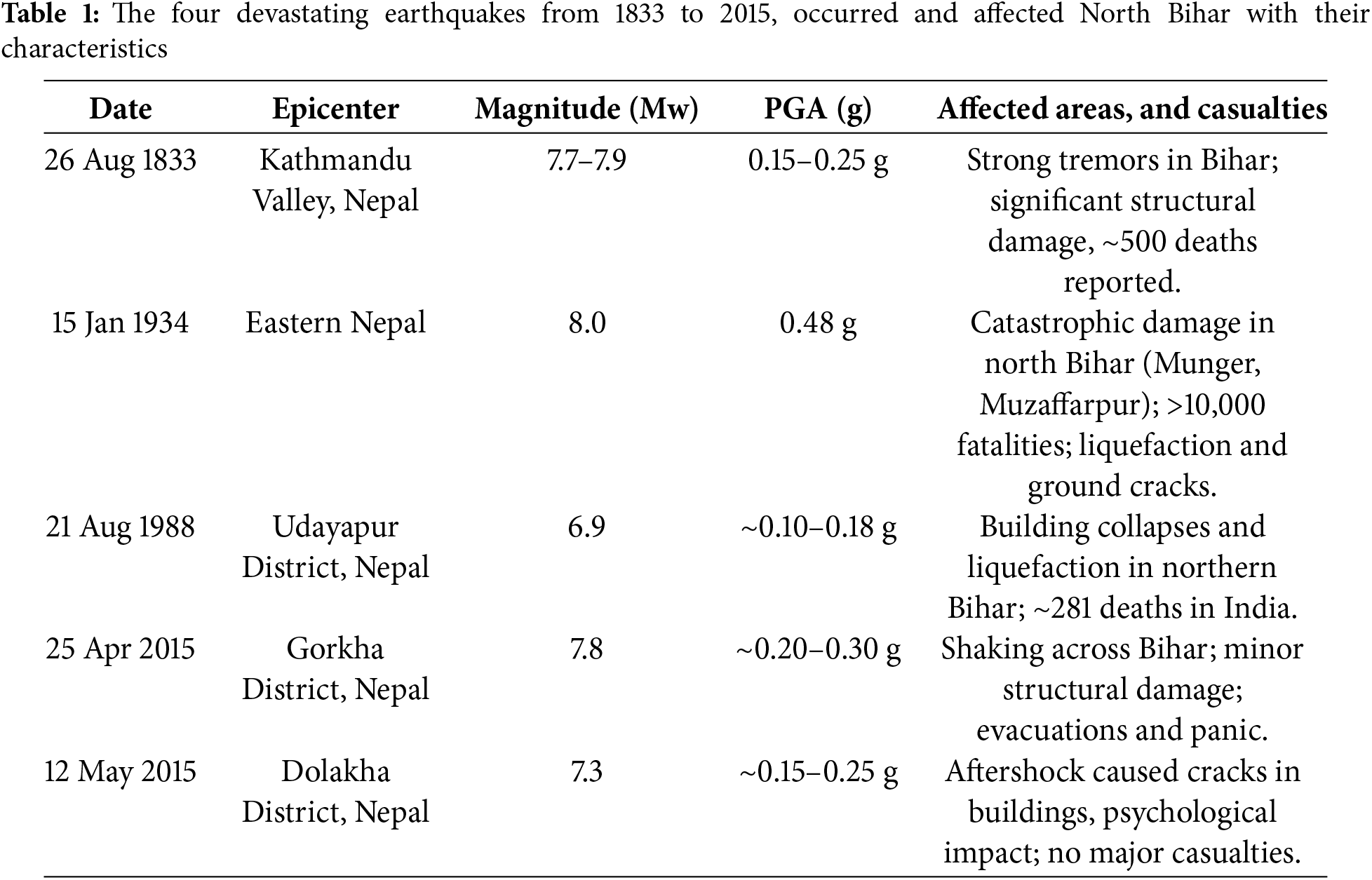
The study area is in the North Bihar region bounded by 27.49°N, 83.81°E to 25.24°N, 88.28°E and is part of the world’s largest alluvial plain, IGP. The IGP has been characterized by several discernible, large scale and micro-scale geomorphic features [32]. Two morpho-stratigraphic units have been recognized in the Indo-Gangetic Plains: the upper Newer Alluvium, also known as the Khadar, and the lower Older Alluvium, also known as the Bhangar or Bangar. Many geological structures and faults, such as the West Patna Fault (WPF), East Patna Fault (EPF), Munger-Saharsa ridge, Gandak fault, etc., are present in the study area. All the faults are spread over North Bihar, and during earthquakes, the structures transfer energy that results in enhanced damage intensity along with the faults. The geological structures influence and control the seismic hazard pattern (Fig. 1).

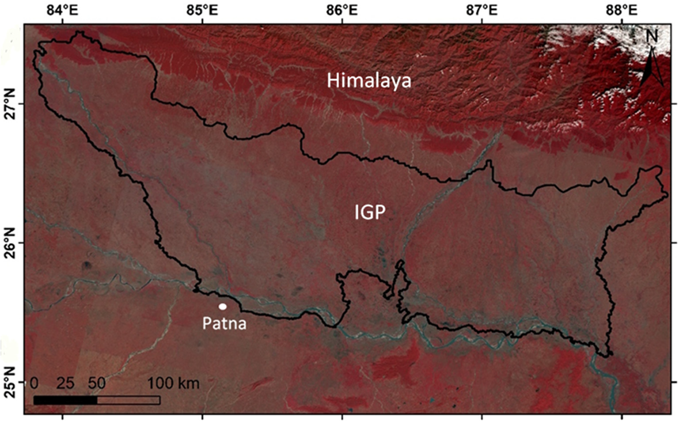
Figure 1: The location of study area shown as False color composites image of Landsat 8 satellite (OLI)

The study area consists of six drainage basins, namely Gandak, Burhi Gandak, Bagmati, Kamla, Kosi, and Mahananda basin. The Gandak and Mahananda basins are very highly active while Kamla basin is relatively least active, and the remaining basins are moderately active. North Bihar has recorded significant liquefaction events during 1934 and 1988 earthquakes.

3  Methodology & Materials Used

3.1 Training Data Selection

This study aims to identify site amplification during earthquakes by analyzing locations of historical earthquake-induced damage. Generally, characteristics of ground shaking are shaped by numerous factors, including seismic source effects, proximity to the fault, local soil conditions, topography, and near-fault influences [33]. Multiple side-specific ground motion models have been developed to predict the seismic source and propagation of seismic wave impact. However the most important and challenging factor is the site effects. Site-specific parameters significantly change locally and influence the hazard distribution. In this work, the sites frequently observing higher damage intensity during previous earthquakes (1934, 1988, 2015 mainshock, and 2015 major aftershock) were considered as training data for training and testing the ML models.

The Modified Mercalli Intensity (MMI) data during the 1934 and 1988 earthquakes were collected from the historical earthquake catalogue. The intensity values for the 2015 Nepal earthquake mainshock and aftershock were extracted using the isoseismal map provided by the United States Geological Survey (USGS), which can be utilized for recent earthquakes. The damaged regions were put together (shown in Fig. 2), and the locations that are common in a minimum of two earthquakes have been recorded and used as training data for ML models.

Figure 2: The Landsat FCC image showing locations of damage sites used as training data for the model, the size of the circles represents damage intensity of individual location in an earthquake

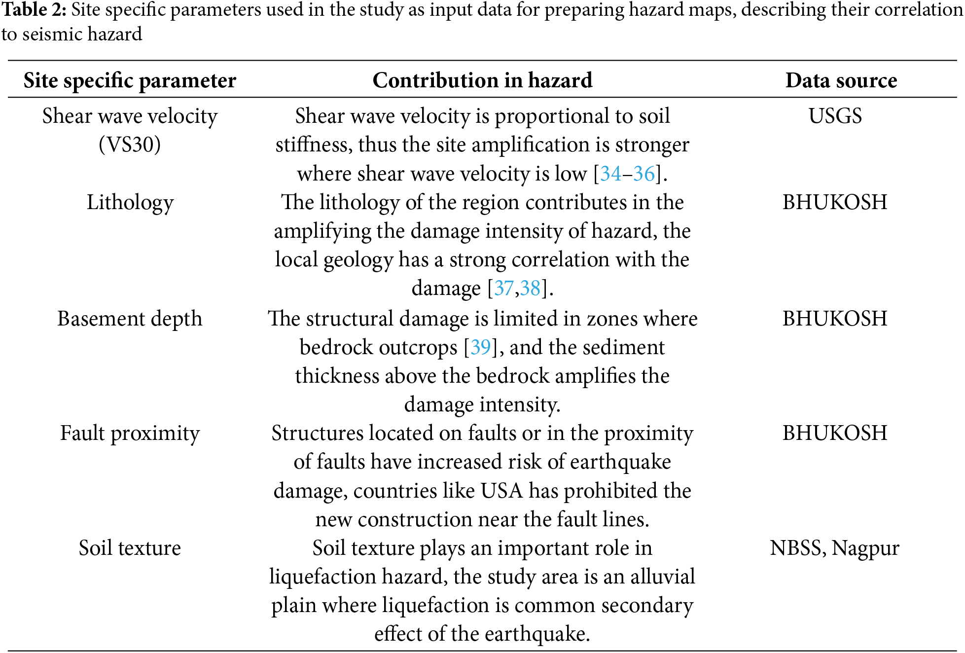
A total number of 152 samples were identified for the analysis, of which 70% were used for training, 15% were used for testing, and the remaining 15% were used for validation purposes. This study considers various site effects, including time-averaged shear wave velocity VS3, soil texture, distance from the fault, bedrock depth, and lithology. Table 2 outlines the relationship between these site-specific parameters and seismic hazard.

3.2 Machine Learning Models

3.2.1 Decision Tree

A Decision Tree can be used for classification as well as regression tasks. It is one of the most important tools in supervised learning algorithms. Tree split algorithms are critical for building decision trees in these approaches, as they rely on quantitative metrics during training to produce an efficient tree structure. The decision tree methodology is frequently employed in data mining to establish classification systems using multiple covariates or to develop prediction algorithms for a target variable. This approach categorizes a population into branch-like segments, forming an inverted tree comprising a root node, internal nodes, and leaf nodes. Being non-parametric, the algorithm adeptly handles large, intricate datasets without necessitating a complex parametric framework. The equation of this algorithm is given below.

Given data Qm available at node m with nm samples and tm as the threshold for node m, the classification and regression tree algorithm for classification may be expressed as follows:

G(Qm,tm)=nmLeftnmH(QmLeft(tm))+nmRightnmH(QmRight(tm))(1)

where H represents the measure of impurities within the left and right subsets at node m, which can be either entropy or Gini impurity. ‘nm’ denotes the count of instances in the left and right subsets at node m.

To select the parameter, we can write as:

tm=tmH(Qm,tm)(2)

3.2.2 K-Nearest Neighbors (KNN)

The simplest classifier available in Machine Learning is the Nearest Neighbor Classifier. It functions by locating the closest neighbors to a given query example and utilizing them to ascertain the class of the query. This classification approach holds significant importance, as concerns regarding slow runtime performance are less prevalent nowadays due to the abundance of computational power available. The KNN classifier, also referred to as an instance-based classifier, operates on the principle that the classification of unknown instances relies on comparing them to known instances using a distance or similar function. Its primary goal is to ensure that instances distant from each other in the instance space, as defined by the appropriate distance function, are less likely to belong to the same class compared to instances situated closer together.

3.2.3 Random Forest

The random forest algorithm proposed by [40] has been extremely successful as a general-purpose classification and regression method. The approach, which combines several randomized decision trees and aggregates their predictions by averaging, has shown excellent performance in settings where the number of variables is much larger than the number of observations. The output of these trees is aggregated into a single output using voting for classification problems or averaging for regression problems (Fig. 3).

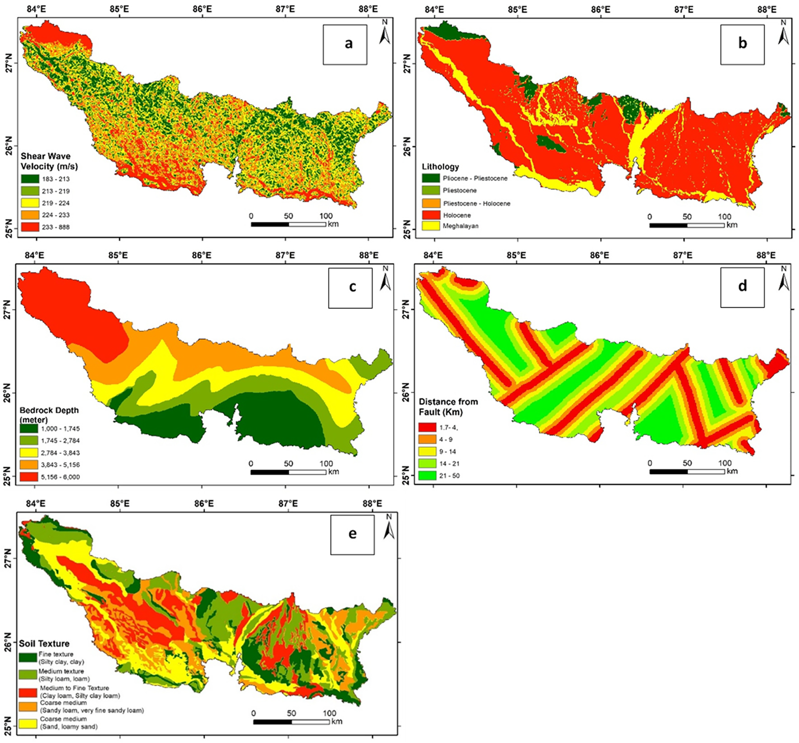
Figure 3: GIS layers of site-specific parameters used as input data for ML models is (a) shear wave velocity, (b) lithology, (c) bedrock depth, (d) distance from fault, and (e) soil texture

3.2.4 Logistic Regression

Logistic regression is a supervised machine learning multivariate statistical approach used for binary classification by predicting the probability of an outcome; the analysis result range falls between 0 and 1 [41]. The model performs analysis over one or other independent parameters to establish a relationship to predict the output in a discrete class. The technique is widely used for the evaluation of the mathematical probability of an event occurring or not. The logistic regression uses a sigmoid function to map predictions and their probabilities. The assumptions considered in the LR model are that the dependable variable should be binary, there should be very low or no multicollinearity between the independent variables, and the LR model requires a large sample size for prediction.

Hyperparameter tuning was carried out using a randomized search combined with 5-fold cross-validation. For each model, we systematically explored a range of critical hyperparameters (e.g., C for logistic regression, max_depth for decision trees, n_neighbors for KNN, and n_estimators for random forests) to determine the optimal configurations. This process was conducted exclusively on the training set, with the final model evaluation performed on a held-out test set to ensure unbiased and reliable comparisons.

3.3 Multicollinearity Analysis

The multicollinearity analysis shown in Table 3 has been performed for the data before applying ML models. The primary assumption for ML models is that the independent parameter should not be correlated or very little correlation should be among these parameters. This analysis shows that all the factors considered for the ML models in this study are not significantly correlated (<0.3) and hence can be used for the model. The multicollinearity in the independent variable reduces the precision of the coefficients, which ultimately weakens the statistical power of the model.

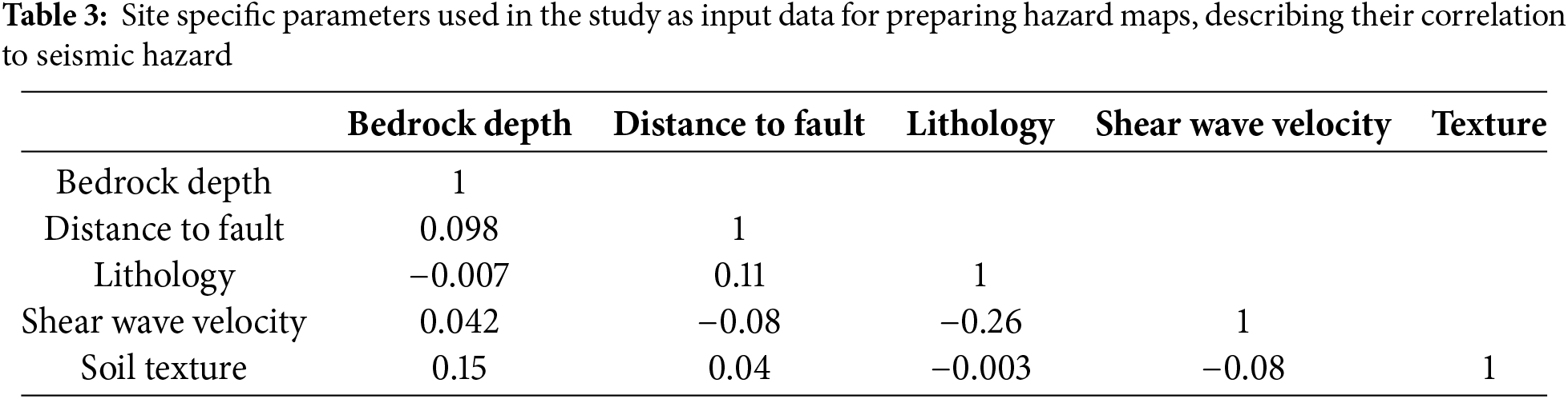
Table 3 presents the multicollinearity analysis of different factors used in hazard map preparation, including Bedrock Depth, Distance to Fault, Lithology, Shear Wave Velocity, and Soil Texture. The correlation coefficients among these factors are all below 0.3, indicating minimal collinearity and ensuring that each parameter contributes uniquely to the model. High multicollinearity can reduce the precision of coefficient estimates, making it difficult to determine the individual impact of variables, which can lead to overfitting and unstable predictions. However, the low correlation values in Table 3 confirm that the chosen parameters do not suffer from significant collinearity, allowing the machine learning models to generate unbiased and stable predictions for seismic hazard assessment. For example, Bedrock Depth and Distance to Fault have a low correlation of 0.098, and the highest observed correlation is 0.15 between Soil Texture and Bedrock Depth, which remains within an acceptable range. This validation ensures that the models perform effectively without distortion from redundant information, ultimately enhancing their statistical power, reliability, and generalizability.

4  Results & Discussion

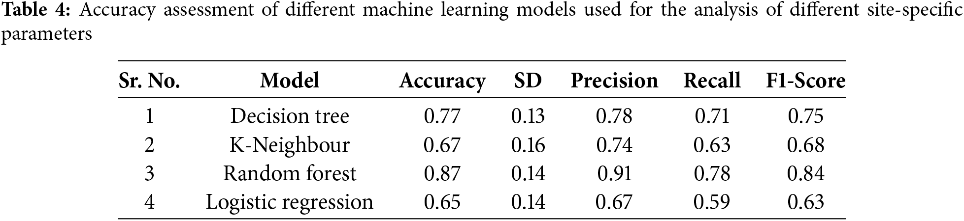
The accuracy of ML models in preparing seismic hazard maps is shown in Table 4. The random forest has obtained maximum accuracy (0.87%), while the LR model has the lowest (0.65%). Random Forest performed better than the other models because it is an ensemble learning method that constructs multiple decision trees and combines their outputs to improve accuracy and reduce overfitting. This approach allows it to capture complex, non-linear relationships between seismic hazard parameters and ground motion, making it particularly effective in hazard assessment. Additionally, Random Forest is robust to multicollinearity and can handle irrelevant or redundant features better than linear models. Since the multicollinearity analysis in Table 3 confirmed that the independent variables had low correlation, Random Forest was able to utilize these diverse inputs effectively to make precise predictions.

The study area, drained by tributaries of the Ganga River such as Gandak, Burhi Gandak, Bagmati, Kamla, Balan, Kosi, and Mahananda are shown in yellow and red patches are visible along the flood plains of the rivers (Fig. 4). The circles 1 and 2 on the hazard map indicate a higher probability of hazard in the northern region where bedrock depth is greater (3500–6000 m), as shown in Fig. 5, suggesting significant sediment thickness. This increased sediment thickness amplifies seismic wave amplitudes, leading to more intense shaking.

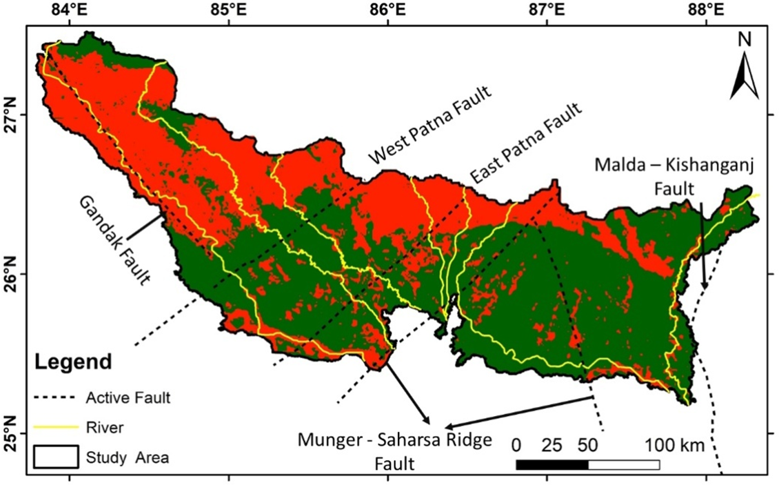
Figure 4: Seismic hazard map of the study area; Yellow lines show tributaries of Ganga River starting from left Gandak, Burhi Gandak, Bagmati, Kamla, Balan, Kosi and Mahananda. The black dashed line shows the active faults crossing the study area

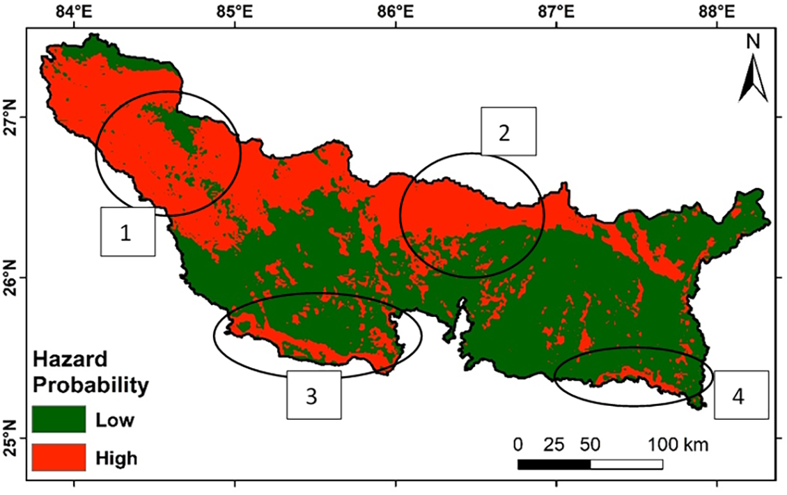
Figure 5: Seismic hazard map showing the location of high probability of hazard, circles 1 and 2 show the region where bedrock depth is deep and sediment thickness is high, circles 3 and 4 show the flood plains of Ganga River where alluvium is unconsolidated hence damage intensity will be more at all the sites

The study area is an alluvial plain, and the shear wave velocity is lower (180–300 m/s) in this region relative to the peninsular India. The site amplification is high where shear wave velocity is low. The flood plains have recent Quaternary alluvium having an unconsolidated nature; hence, the seismic wave takes a longer time to travel, which increases the amplitude of seismic waves during earthquakes, resulting in strong shaking. For illustration, during the Bhuj earthquake in 2001, the epicenter was situated 330 km from Ahmedabad city, and due to the unconsolidated sedimentary cover of the Sabarmati river in Ahmedabad, soil amplification was recorded, resulting in strong shaking followed by heavy damage [42].

The active faults were overlaid on the hazard map (Fig. 4), and the prominent red patches were observed along with the active faults. Along the West Patna Fault (WPF) and East Patna Fault (EPF), a higher probability (red patches) is visible; EPF is responsible for the 1934 and 1988 earthquakes [43]. The probability of hazard intensity along the Ganga River near Patna and Munger is high, as depicted by circles 3 and 4 (Fig. 5). In the 1934 Bihar-Nepal earthquake, the Munger region recorded heavy damage, and the damage intensity was X on the MMI classification in this region. Damage intensity from Munger to Patna was confined to a small strip along the Ganga River and its floodplain [44].

5  Conclusion

This study assessed seismic hazards and analyzed damage patterns influenced by regional geological and topographical factors. The findings indicate that site-specific parameters, such as soil characteristics, lithology, and proximity to geological features, are critical in understanding seismic hazard distribution. The seismic hazard map developed in this study highlights increased hazard potential along rivers, floodplains, active faults, and areas with significant sediment thickness.

Based on these results, it is recommended that settlement areas be planned away from these high-risk geological features to mitigate potential damage. The insights gained from this study can aid urban planners in formulating strategies for sustainable land use, infrastructure development, and hazard-resilient construction. Additionally, the findings are valuable for optimizing the distribution of residential and commercial zones, managing utilities, and selecting suitable sites for critical infrastructure such as nuclear power plants, thereby reducing the risk of catastrophic damage in future seismic events.

In this study, crucial parameters such as earthquake magnitude and the resulting PGA were not considered despite their significance. In future research, these parameters will be incorporated to enhance the robustness of the hazard maps.

Acknowledgement: Not applicable.

Funding Statement: The authors received no specific funding for this study.

Author Contributions: Abhishek Rawat has conceptualized the work, Shilpa Suman and Harsh Kumar have done the data preparation and interpretation, Rajat Subhra Chatterjee, Dheeraj Kumar and B. S. Chaudhary have reviewed the manuscript and edited. All authors reviewed the results and approved the final version of the manuscript.

Availability of Data and Materials: Most of the data is available on different portals and the generated data will be available on reasonable requests.

Ethics Approval: Not applicable.

Conflicts of Interest: The authors declare no conflicts of interest to report regarding the present study.

References

1. Wesnousky SG. Great pending Himalaya earthquakes. Seismol Res Lett. 2020;91(6):3334–42. doi:10.1785/0220200200. [Google Scholar] [CrossRef]

2. Keshri CK, Mohanty WK, Ranjan P. Probabilistic seismic hazard assessment for some parts of the Indo-Gangetic plains, India. Nat Hazards. 2020;103(1):815–43. doi:10.1007/s11069-020-04014-8. [Google Scholar] [CrossRef]

3. Parkash B, Kumar S, Rao MS, Giri SC, Kumar CS, Gupta S, et al. Holocene tectonic movements and stress field in the western Gangetic plains. Curr Sci. 2000;79(4):438–49. [Google Scholar]

4. Thakur VC, Pandey AK. Active deformation of Himalayan Frontal Thrust and piedmont zone south of Dehradun in respect of seismotectonics of Garhwal Himalaya. Himal Geol. 2004;25(1):23–31. [Google Scholar]

5. Bhosle B, Parkash B, Awasthi AK, Singh VN, Singh S. Remote sensing-GIS and GPR studies of two active faults, Western Gangetic Plains. India J Appl Geophys. 2007;61(2):155–64. doi:10.1016/j.jappgeo.2006.10.003. [Google Scholar] [CrossRef]

6. Yeats RS, Thakur VC. Active faulting south of the Himalayan front: establishing a new plate boundary. Tectonophysics. 2008;453(1–4):63–73. doi:10.1016/j.tecto.2007.06.017. [Google Scholar] [CrossRef]

7. Goswami PK. Controls of basin margin tectonics on the morphology of alluvial fans in the western Ganga foreland basin’s piedmont zone. India Geol J. 2018;53(5):1840–53. doi:10.1002/gj.3010. [Google Scholar] [CrossRef]

8. Malik JN, Shah AA, Sahoo AK, Puhan B, Banerjee C, Shinde DP, et al. Active fault, fault growth and segment linkage along the Janauri anticline (frontal foreland foldNW Himalaya, India. Tectonophysics. 2010;483(3–4):327–43. doi:10.1016/j.tecto.2009.10.028. [Google Scholar] [CrossRef]

9. Pati P, Parkash B, Awasthi AK, Acharya V. Holocene tectono-geomorphic evolution of parts of the Upper and Middle Gangetic plains, India. Geomorphology. 2011;128(3–4):148–70. doi:10.1016/j.geomorph.2011.01.001. [Google Scholar] [CrossRef]

10. Nath S, Chatterjee RS, Mohanty SP, Gaurav S. Comparative evaluation of active tectonics in parts of the frontal region of NW Himalaya, India by geomorphic analysis and geophysical investigation. J Geol Soc Ind. 2019;94(2):197–205. doi:10.1007/s12594-019-1289-3. [Google Scholar] [CrossRef]

11. Kumar H, Chatterjee RS, Patel RC, Rawat A, Nath S. Geomorphic mapping and analysis of neotectonic structures in the piedmont alluvial zone of Haryana state, NW-India: a remote-sensing and GPR based approach. Geomat Nat Hazards Risk. 2023;14(1):2221371. doi:10.1080/19475705.2023.2221371. [Google Scholar] [CrossRef]

12. Safari HO, Pirasteh S, Pradhan B, Gharibvand LK. Use of remote sensing data and GIS tools for seismic hazard assessment for shallow oilfields and its impact on the settlements at Masjed-i-Soleiman area, Zagros Mountains, Iran. Remote Sens. 2010;2(5):1364–77. doi:10.3390/rs2051364. [Google Scholar] [CrossRef]

13. Dal Zilio L, Hetényi G, Hubbard J, Bollinger L. Building the Himalaya from tectonic to earthquake scales. Nat Rev Earth Environ. 2021;2(4):251–68. doi:10.1038/s43017-021-00143-1. [Google Scholar] [CrossRef]

14. Bilham R. Location and magnitude of the 1833 Nepal earthquake and its relation to the rupture zones of contiguous great Himalayan earthquakes. Curr Sci. 1995;69(2):101–28. [Google Scholar]

15. Nath SK, Thingbaijam KKS. Probabilistic seismic hazard assessment of India. Seismol Res Lett. 2012;83(1):135–49. doi:10.1785/gssrl.83.1.135. [Google Scholar] [CrossRef]

16. National Disaster Management Authority. Development of probabilistic seismic hazard map of India [Internet]. [cited 2025 Jun 8]. Available from: https://www.geophysik.uni-muenchen.de/~kaeser/Literature/PSHAmap_India_2010.pdf. [Google Scholar]

17. Das S, Gupta ID, Gupta VK. A probabilistic seismic hazard analysis of Northeast India. Earthq Spectra. 2006;22(1):1–27. doi:10.1193/1.2163914. [Google Scholar] [CrossRef]

18. Mahajan AK, Thakur VC, Sharma ML, Chauhan M. Probabilistic seismic hazard map of NW Himalaya and its adjoining area, India. Nat Hazards. 2010;53(3):443–57. doi:10.1007/s11069-009-9439-3. [Google Scholar] [CrossRef]

19. Anbazhagan P, Bajaj K, Matharu K, Moustafa SSR, Al-Arifi NSN. Probabilistic seismic hazard analysis using the logic tree approach-Patna district (India). Nat Hazards Earth Syst Sci. 2019;19(10):2097–115. doi:10.5194/nhess-19-2097-2019. [Google Scholar] [CrossRef]

20. Sinha R, Sarkar R. Deterministic seismic hazard assessment of Dhanbad City, India. In: Proceedings of the 7th International Conference on Recent Advances in Geotechnical Earthquake Engineering and Soil Dynamics; 2021 Jul 12–15; Bangalore, India. [Google Scholar]

21. Ahmed T, Rehman K, Shafique M, Ali W. GIS-based earthquake potential analysis in Northwest Himalayan. Pakistan Environ Earth Sci. 2023;82(4):1–19. doi:10.1007/s12665-023-10798-2. [Google Scholar] [CrossRef]

22. Dey S, Das S, Saha A. Exploring uncertainty analysis in GIS-based landslide susceptibility mapping models using machine learning in the Darjeeling Himalayas. Earth Sci Inform. 2025;18(1):42. doi:10.1007/s12145-024-01561-7. [Google Scholar] [CrossRef]

23. Jena R, Pradhan B, Beydoun G, Alamri AM, Sofyan H. Earthquake hazard and risk assessment using machine learning approaches at Palu, Indonesia. Sci Total Environ. 2020;749(1):141582. doi:10.1016/j.scitotenv.2020.141582. [Google Scholar] [PubMed] [CrossRef]

24. Pancholi V, Bhatt N, Singh P, Chopra S. Multi-criteria approach using GIS for macro-level seismic hazard assessment of Kachchh Rift Basin, Gujarat, western India—first step towards earthquake disaster mitigation. J Earth Syst Sci. 2022;131(1):3. doi:10.1007/s12040-021-01744-6. [Google Scholar] [CrossRef]

25. Saha A, Tripathi L, Villuri VGK, Bhardwaj A. Exploring machine learning and statistical approach techniques for landslide susceptibility mapping in Siwalik Himalayan Region using geospatial technology. Environ Sci Pollut Res Int. 2024;31(7):10443–59. doi:10.1007/s11356-023-31670-7. [Google Scholar] [PubMed] [CrossRef]

26. Suman S, Kumar A, Kumar D, Soni A. Augmenting possibilistic c-means classifier to handle noise and within class heterogeneity in classification. J Appl Remote Sens. 2021;15(4):1–17. doi:10.1117/1.jrs.15.044509. [Google Scholar] [CrossRef]

27. Anbazhagan P, Kumar A, Sitharam TG. Seismic site classification and correlation between standard penetration test N value and shear wave velocity for Lucknow City in Indo-Gangetic Basin. Pure Appl Geophys. 2013;170(3):299–318. doi:10.1007/s00024-012-0525-1. [Google Scholar] [CrossRef]

28. Bilham R. Himalayan earthquakes: a review of historical seismicity and early 21st century slip potential. Geol Soc Lond Spec Publ. 2019;483(1):423–82. doi:10.1144/sp483.16. [Google Scholar] [CrossRef]

29. Martin S, Szeliga W. A catalog of felt intensity data for 570 earthquakes in India from 1636 to 2009. Bull Seism Soc Am. 2010;100(2):562–9. doi:10.1785/0120080328. [Google Scholar] [CrossRef]

30. Rawat A, Kumar D, Chatterjee RS, Kumar H. A GIS-based liquefaction susceptibility mapping utilising the morphotectonic analysis to highlight potential hazard zones in the East Ganga plain. Environ Earth Sci. 2022;81(13):1–16. doi:10.1007/s12665-022-10468-9. [Google Scholar] [CrossRef]

31. Rawat A, Kumar D, Chatterjee RS, Kumar H. Reconstruction of liquefaction damage scenario in Northern Bihar during 1934 and 1988 earthquake using geospatial methods. Geomat Nat Hazards Risk. 2022;13(1):2560–78. doi:10.1080/19475705.2022.2122591. [Google Scholar] [CrossRef]

32. Singh IB. Late quaternary history of the Ganga plain. J Geol Soc Ind. 2004;64(4):431–54. [Google Scholar]

33. Rathje EM, Bachhuber J, Dulberg R, Cox BR, Kottke A, Wood C, et al. Damage patterns in port-au-prince during the 2010 Haiti earthquake. Earthq Spectra. 2011;27(1_suppl1):117–36. doi:10.1193/1.3637056. [Google Scholar] [CrossRef]

34. Sundararajan N, Seshunarayana T. Liquefaction hazard assessment of earth quake prone area: a study based on shear wave velocity by multichannel analysis of surface waves (MASW). Geotech Geol Eng. 2011;29(3):267–75. doi:10.1007/s10706-010-9360-2. [Google Scholar] [CrossRef]

35. Sundararajan N, El-Hussain I, Mohamed AME, Deif A, El-Hady S, El-Jabri K, et al. Shear wave velocity characteristics in parts of Muscat, sultanate of Oman—a measure of earthquake hazard assessment. J Geol Soc Ind. 2019;93(5):515–22. doi:10.1007/s12594-019-1212-y. [Google Scholar] [CrossRef]

36. Boore DM. Estimating s(30) (or NEHRP site classes) from shallow velocity models (depths < 30 m). Bull Seism Soc Am. 2004;94(2):591–7. doi:10.1785/0120030105. [Google Scholar] [CrossRef]

37. Spudich P, Hellweg M, Lee WHK. Directional topographic site response at Tarzana observed in aftershocks of the 1994 Northridge, California, earthquake: implications for mainshock motions. Bull Seism Soc Am. 1996;86(1B):S193–208. doi:10.1785/bssa08601bs193. [Google Scholar] [CrossRef]

38. Ayele A, Woldearegay K, Meten M. A review on the multi-criteria seismic hazard analysis of Ethiopia: with implications of infrastructural development. Geoenviron Disasters. 2021;8(1):9. doi:10.1186/s40677-020-00175-7. [Google Scholar] [CrossRef]

39. Bol E. Determination of the relationship between soil properties and earthquake damage with the aid of neural networks: a case study in Adapazari, Turkey. Nat Hazards Earth Syst Sci. 2012;12(9):2965–75. doi:10.5194/nhess-12-2965-2012. [Google Scholar] [CrossRef]

40. Breiman L. Random forests. Mach Learn. 2001;45(1):5–32. doi:10.1023/A:1010933404324. [Google Scholar] [CrossRef]

41. Althuwaynee OF, Pradhan B, Park HJ, Lee JH. A novel ensemble bivariate statistical evidential belief function with knowledge-based analytical hierarchy process and multivariate statistical logistic regression for landslide susceptibility mapping. Catena. 2014;114(1):21–36. doi:10.1016/j.catena.2013.10.011. [Google Scholar] [CrossRef]

42. Narayan JP, Sharma ML. Effects of local geology on damage severity during Bhuj, India earthquake. In: Proceedings of the 13th World Conference on Earthquake Engineering; 2004 Aug 1–6; Vancouver, BC, Canada. [Google Scholar]

43. Verma AK, Pati P, Sharma V. Soft sediment deformation associated with the East Patna Fault south of the Ganga River, northern India: influence of the Himalayan tectonics on the southern Ganga plain. J Asian Earth Sci. 2017;143:109–21. doi:10.1016/j.jseaes.2017.04.016. [Google Scholar] [CrossRef]

44. Kayal JR. Seismotectonics of the great and large earthquakes in Himalaya. Curr Sci. 2014;106(2):188–97. [Google Scholar]