Statistical and Visual Evaluation of Artificial Neural Networks and Multiple Linear Regression Performances in Estimating Reference Crop Evapotranspiration for Mersin

1  Introduction

Reference Crop Evapotranspiration (ETo) is presented to investigate the evaporation demand of the atmosphere regardless of plant type, plant growth, or management practices. Therefore, ETo, which represents the evaporation power of the atmosphere, can be determined at a specific location at any time of the year, regardless of plant or soil characteristics.

It is calculated with the help of a lysimeter, empirical models such as Baier-Robertson, Hargreaves, and Penman-Monteith, and statistical models such as regression, artificial neural networks, and random forest [1–3]. Some studies have examined the spatial and temporal distribution [4], historical accumulation of crop evapotranspiration due to climate change in Bangladesh [5], the seasonal impact of climate change [6], crop evaporation values, and irrigation schedules [7]. The climate dataset must be complete to use the Penman-Monteith method, which is the ideal approach, and calculate the ETo value. ETo can be calculated using techniques such as the Hargreaves equation [8] or linear interpolation for incomplete climate data. It has been observed that ETo is calculated using tree-based regression and deep learning-based gated recurrent unit (GRU) models with restricted climate datasets [9]. Climate datasets were measured decently in most regions between 1983 and 2017 in the Bangladesh study region; therefore, ETo prediction was made using Bagging, RF, RS, RT and SVM methods [10]. In cases where all datasets were unavailable, the Adaptive Neuro-Fuzzy Inference System (ANFIS) computer module was used again [11].

Artificial intelligence techniques are popular for generating quick solutions to problems. The PM method, other empirical models, and statistical models for ETo estimation were used for comparisons. In the literature, study area, number of stations, time interval, climate data, and quantity vary. All measurable climate data or combinations were considered as input and ETo output, and models were developed with the best model being tried to be put forward by applying two or more methods. In addition to ETo estimation, the ANN method is used in estimating climate data such as Max temperature, Min temperature, Relative Humidity, Wind speed, Sunshine, Dew Point, and Evaporation [12]. Researchers have tested many statistical methods individually or in combination through comparisons and analyses. Modern methods such as Multiple Linear Regression (MLR) [13–16], Artificial Neural Network (ANN) [17,18], Random Forest (RF) [19,20], Genetic Algorithm [21], K-means Clustering and firefly algorithms [22], Support Vector Machine (SVM), Firefly algorithm (FFA) [23], Multivariate Adaptive Regression Splines (MARS) [24], and hybrid methods such as Adaptive Network-Based Fuzzy Inference System (ANFIS) [25–29], Generalized Regression Neural Network [30,31], hybrid-deep learning approach [32], and Extreme Learning Machines [33,34] are seen to be applied. There are numerous versions, particularly in studies that use ANN and hybrid methods. For example, ETo was calculated using recurrent neural networks (RNNs), namely long short-term memory (LSTM) and bidirectional LSTM [35–38]; Artificial Neural Network/Backpropagation Algorithm [39,40]; deep learning neural network (DLNN), multilayer perceptron (MLP) [41], and radial basis function neural network (RBFNN) [42], as machine learning and deep learning methods RF, XGBoost, Artificial Neural Network (ANN) and convolutional neural network (CNN) [19,43]; support vector regression (SVR), regression trees (RT), linear regression, k-nearest neighbors, Bayes networks, logistic regression, K* algorithm [44]; RF, Generalized regression neural network (GRNN) and CatBoost based on gradient boosting decision tree (GBDT) [45,46], Light Gradient Boosting Model [47], novel improved Grey Wolf Algorithm [48,49], whale optimization algorithm [34,50] and compared with traditional PM method. AI models are hybrid SVR-GWO models, hybrid SVR-genetic algorithms (SVR-GA), SVR-particle swarm optimizers (SVR-PSO), conventional artificial neural network (ANN), and using empirical models (Turc, Ritchie, Thornthwaite, and three versions of Valiantzas methods), ETo estimates were made on a multi-time scale [51]. In addition, a hybrid, least-square support vector regression with a gravitational search algorithm (LSSVR-GSA) and the dynamic evolving neural-fuzzy inference system (DENFIS) were used and compared with the M5 model tree (M5RT) approach [52].

The aim of the present study was to develop modern crop evapotranspiration (ETo) methods using different variables and datasets in Mersin province based on the Penman-Monteith method. In this direction, the 31-day climate data of May, belonging to the years 2015–2020, of a total of 36 stations were used. The novelty of the present study is the calculation of ETo, regionally and daily, for single and all AWOS with the data of May in the years 2015–2020, creating six models from three scenarios with MLR and ANN methods using fewer criteria than PM, and visualizing them with maps. For the estimation of plant water consumption, the Penman-Monteith method was coded in the Python programming language and was considered a benchmark for the comparison of modern methods to be used in the study. We produced a prediction model for the climate data of 36 stations, both separately and collectively, using the statistical methods of regression and ANN. Namely, each station’s data were analyzed individually and collectively to evaluate the prediction models at the same time, variable, and data. The R-Squared (R2), the Mean Absolute Error (MAE), the Mean Absolute Percentage Error (MAPE), and the Root Mean Square Error (RMSE) values were compared in the performance analysis. A connection was established between the ETo values and the station using a Geographical Information System (GIS). Maps were obtained using Inverse Distance Weighted (IDW), a spatial analysis method, and the results were interpreted visually. In addition, unlike other studies, it focused on the short term only. This was done to evaluate the effect of the extraordinary increase in temperature and wind on the plant water requirements during the working dates. Especially Mersin, which is the leading city in lemon cultivation in the world, has been greatly affected by this. It has been proved by the ETo calculations and estimation results that the plant water consumption has increased in parallel with the consideration of May when the temperature is above the seasonal normal. This study is intended to serve as a guide for future research. In this context, it will serve as a reference for future research to calculate month-day ETo across all seasons using diverse meteorological data and various artificial intelligence methods, and utilize remote sensing data in estimating ETo of extensive areas.

2  Materials and Methods

2.1 Study Area Study Area and Dataset Creation

Mersin province, in Turkey’s Mediterranean Region, is located between 36∘−37∘ north latitudes and 33∘−35∘ east longitudes. Mersin province has a topographic structure (Digital Elevation Model-DEM) that begins at zero meters above sea level and rises to approximately three thousand meters (Fig. 1). In the last year, the province of Mersin, like the rest of the world and Turkey, has experienced droughts, with areas drying up or water scarcity due to excessive and unconscious water consumption [53]. The irrigation process in the lemon orchard begins in April and May, and the demand for water increases in summer. Mersin had 48 percent of the lemon orchards in 2019 and is the leading exporter [54]. Due to the widespread cultivation of lemons in Mersin Province, it was considered a representative crop in this study. Lemon trees are among the citrus species that are highly sensitive to climatic conditions and have notable sensitivity to water requirements. This characteristic enhances the relevance and practical applicability of reference evapotranspiration (ETo) calculations, making lemons a methodologically meaningful choice for this study.

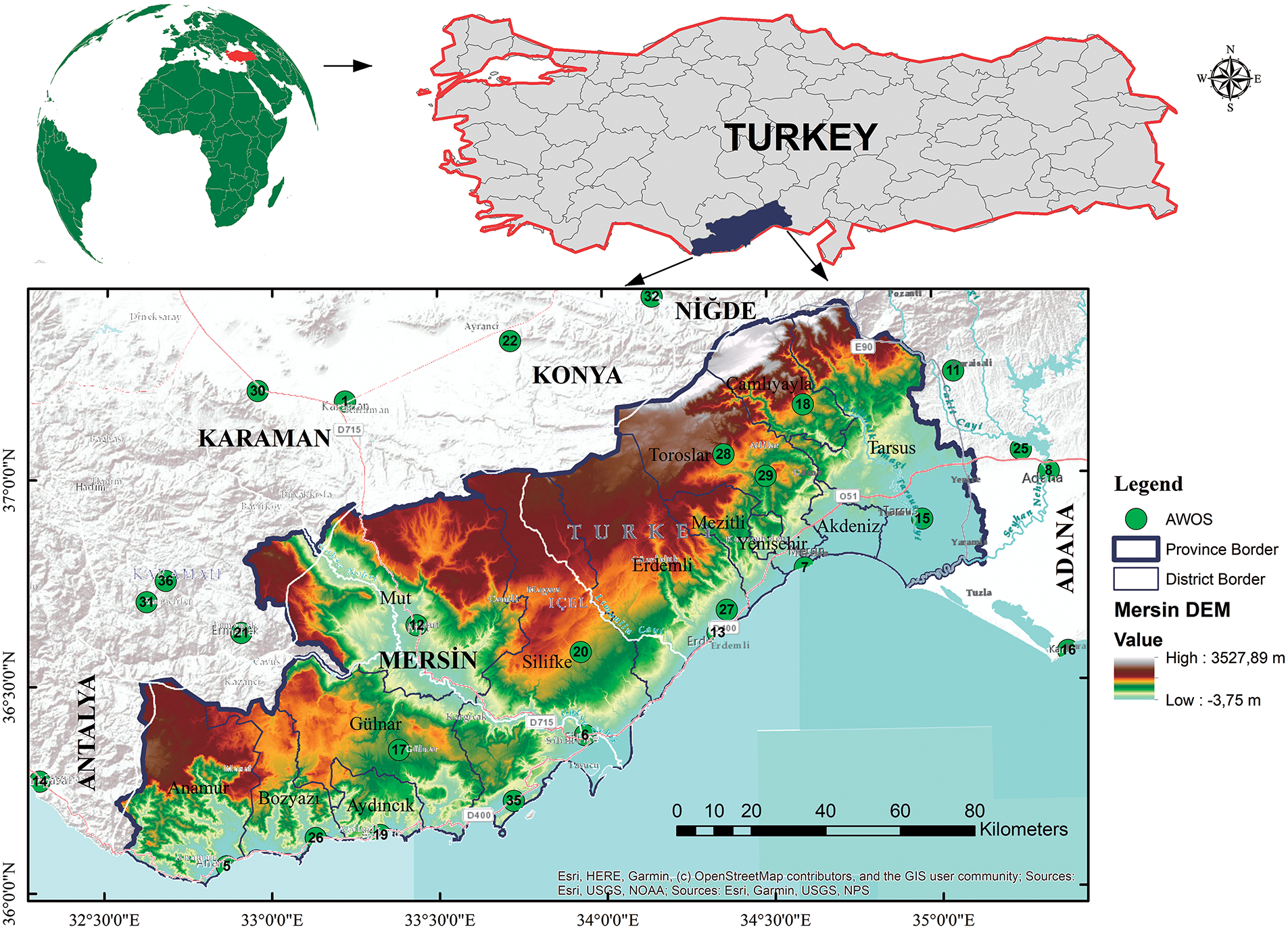
Figure 1: Topography of the study area and AWOS

In Mersin province, the Turkish State Meteorological Service is responsible for the Automated Weather Observing System (AWOS), which includes a total of 39 meteorological stations—34 located on land and five as buoys in the sea. Only 15 of 39 stations had anemometers that measured wind speed. Wind speed is a climatic data element and an important variable in PM calculation. For this reason, only 15 stations were used in the study for Mersin province. In addition to the 15 stations, 21 stations in neighboring provinces were utilized to correctly perform the statistically Inverse Distance Weighting (IDW) interpolation of ETo maps process with exhibiting a balanced dispersion. The locations of the 36 station points used in the present study are pointed out by numbering on the map as green circles (Fig. 1).

Office software was used on a regular basis to prepare data for analysis. MLR analysis was performed using the IBM SPSS Statistics 20 Version software package. It is useful software to build predictive models and uncover complex relationships [55]. Codes created in Matlab R2010b were used for ANN analysis. Matlab blends a programming language that expresses matrix and array mathematics with an environment optimized for iterative analysis and design processes [56]. The study diagram presents all of the processes carried out in the current study (Fig. 2).

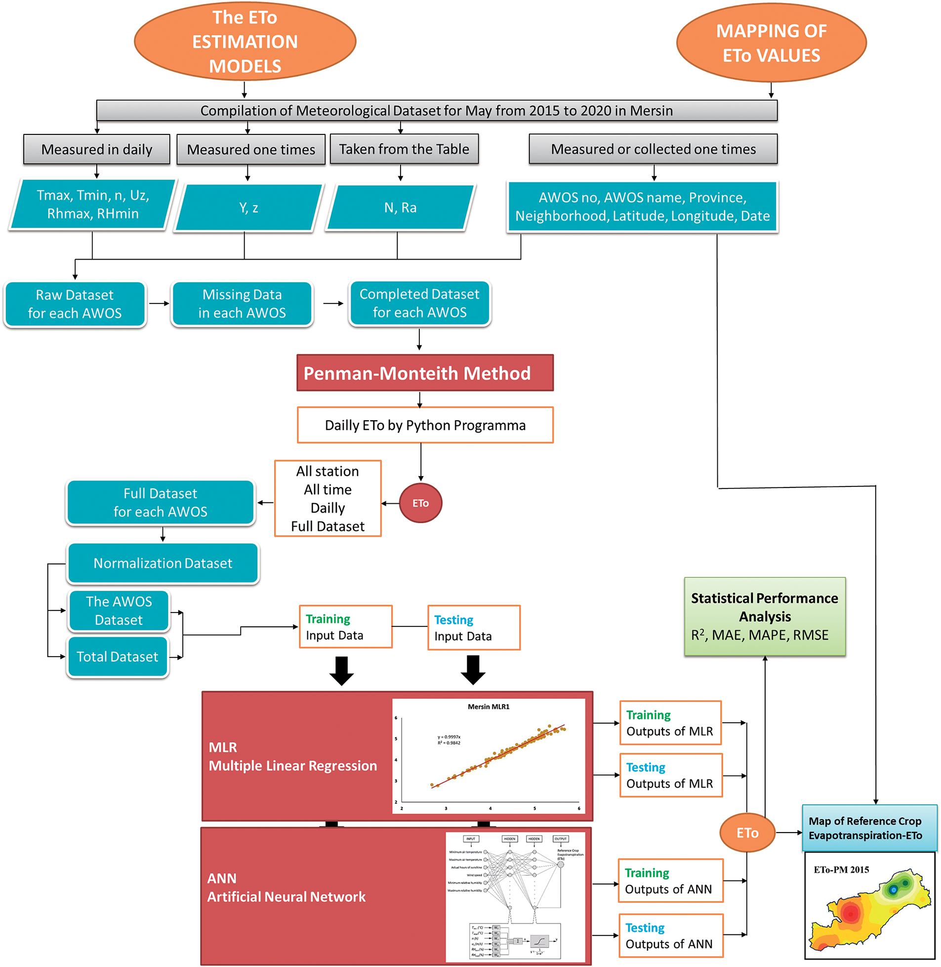
Figure 2: The study diagram for statistical and visual evaluation of ETo

2.2 Reference Crop Evapotranspiration Calculation Methods

2.2.1 Empirical Model: Penman-Monteith Method

Empirical models were developed based on temperature and radiation. The Penman-Monteith (PM) approach, broadly recognized as closely approximating reality, is one of these methods. The United Nations Food and Agriculture Organization concluded that the Penman-Monteith technique is more appropriate for a transparent and uniform globally computation of ETo. The PM technique is referred to as FAO56 Penman-Monteith (FAO PM56) in Paper No. 56, issued in 1998 [8]. This study aimed to standardize the derivation of the reference evapotranspiration equation and enhance the transferability of the plant coefficients. Scientists, engineers, judges, legislators, and end-users have conceptualized a universally recognized equation. They claimed that the equation applies to agricultural and landscape irrigation, making it easier to use and transfer plant and landscape coefficients [57].

The PM method, which is also accepted and foreseen by the FAO, is the most preferred and only standard worldwide [8,57–59]. The methodology established by Penman and Monteith comprises 18 interrelated equations (Appendices A and B). The FAO Penman–Monteith equation (Eq. (1)), as detailed in the FAO Irrigation and Drainage Paper, was employed to calculate reference evapotranspiration (ETo) [8].

ETo=0.408Δ(Rn−G)+γ900T+273u2(es−ea)Δ+γ(1+0.34u2)(1)

The diagram below shows the equivalents of the expressions in FAO Penman-Monteith Eq. (1) (Table 1). Additionally, we calculated each variable using the corresponding equations presented in Appendix B to obtain the necessary input values for Eq. (1). The letter symbols and definitions of these variables are detailed in Appendix A.

2.2.2 Statistical Models

Penman-Monteith ETo values (EToPM), which were taken as benchmarks for the MLR and ANN models, were calculated. Daily ETo was calculated using coding and a total of ten variables, including Tmax,Tmin,n,uz,RHmax,RHmin,z,Y,N and Ra in the PM Eq. (1). Three scenarios were created using climate data in the PM method to estimate the ETo value statistically. Scenario 1: MLR1 and ANN1 analyses for individual stations; Scenario 2: MLR2 and ANN2 analyses for combined stations Tmax,Tmin,n,uz,RHmax, and RHmin a total of six variables; and Scenario 3: For stations with combined MLR3 and ANN3 analyses, Y and N data were added to the file and datasets with a total of eight variables were created (Table 2). The primary aim of the scenarios presented in Table 2 is to achieved the most accurate estimation with the least number of input variables. This approach is particularly important due to the practical limitations associated with meteorological data, such as missing records, the cost and effort of data acquisition, and the variability in station data availability and reliability. In Scenarios 1 and 2, the same set of variables was used; however, Scenario 1 analyzed the stations individually, while Scenario 2 analyzed them collectively. This structural difference highlights the impact of spatial data integration on the model performance. Scenario 3, on the other hand, differed from the first two by incorporating a larger number of variables, aiming to explore the effect of enhanced input richness on the accuracy of the ETo estimation. These models were created by analyzing the data according to scenarios, and by estimating the ETo value, the models were compared using both error rates and maps.

The height at which the wind was measured (z) at all stations was 10 m, and it had the same value. The altitudes of the station points above sea level (Y) are the same within themselves when the stations are analyzed separately, but they vary for each station point in the combined dataset. Because the latitudes of the station points do not vary much, the value varies little, but the value does not change and is the same for all station points. While each station is analyzed individually, since the data is the same, they are excluded from the analysis and must therefore be ignored. Only values were ignored when analyzing the combined data as a whole. As a result, the variable numbers in the column of the dataset organized in a matrix format were clarified. Table 2 shows the schedules of scenarios for the models according to the ETo estimation methods, type of estimation method, and meteorological data (dependent variables).

Multiple Linear Regression Analysis

Regression analysis is a statistical tool for investigating variables [60]. Statistical models are produced to reflect an event or any object aspect and are adapted for various reasons. The aim of regression analysis is to build mathematical models that describe or explain relationships that exist between independent variables [61]. A model is created by finding coefficients using the least squares method. With the help of the model in Eq. (2), the dependent variable y′ can be estimated. The difference (implus) between the actual observation value (yi) and the estimated value (yi^) is the amount of error expressed (ϵ) as a residual. In theory, the residuals sum to zero. In practice, the sum may not be exactly zero due to rounding. The sum of the residuals in any regression problem is always zero when there is a β0 term in the model as a consequence of the first normal equation. The closer the points are to the Regression Line of the point distributions plotted on the x-y axes of the actual observation value (yi) and predicted value (yi^), the more accurate the model [62]. Multiple regression analysis is used to obtain the correct result by using more than one variable, and its mathematical model is as shown in Eq. (2) [60,62,63].

y=β0+β1x1+β2x2+…+βkxk+ϵ(2)

Eq. (2) explanation of the mathematical model [63]:

x1,x2,…,xk: Independent variables [maximum and minimum air temperature (Tmax and Tmin), actual hours of sunshine (n), wind speed measured at z m height (uz), maximum and minimum relative humidity (RHmax) and RHmin]

y: Dependent variable [Reference crop evapotranspiration (ETo)]

β0,β1,β2,…,βk: The coefficients, estimated by the method of least squares

ϵ: Margin of error (ϵ = the residual =yi−yi^)

It is understood from ANOVA and the F-statistic whether the regression model is significantly explained by the independent variables. As a result of ANOVA, if the F value is p < 0.05, the significance level is checked. It aids in determining whether the model is appropriate and contributes significantly to the explanation of the model’s dependent variable. The R2 value expresses what percentage of the variance in the dependent variable can be explained by the independent variable [64]. R2 takes a value between zero and one. A high R2 value indicates that the regression model explains the variation in the dependent variable well [60].

In the present study, regression analysis was used to describe the relationship between independent variables, such as maximum and minimum air temperature, actual hours of sunshine, wind speed, and maximum and minimum relative humidity, as well as to predict the ETo dependent variable.

Artificial Neural Network

The nervous system in the human brain is stimulated by the artificial neural network. Learning is accomplished by varying the strengths of synaptic connections between neurons [65]. Artificial neural networks, which are made up of a complex network structure of artificial neurons, function similarly to the workings of the human brain [66,67]. These neurons process the input data and calculate the weights before running the activation function and determining the output [65].

A wide variety of architectures exist, starting from a simple single-layer perceptron to complex multilayer networks [65]. “There are connections back from the output neurons to the input neurons, and as such the network holds in memory of its previous states and the next state depends on current input signals and the previous states of the network.” [67]. It can consist of a single layer of neurons with each neuron feeding its output signal back to the inputs of all the other neurons [68,69]. The most widely utilized activation functions in ANN are linear and sigmoid (Eq. (3)) functions [41,70,71]. Because the ETo value is included in the ANN analysis, the network is trained using supervised learning. The present study employed feedback, and given that the activation function data falls between 0 and 1, the sigmoid function is the preferred choice (Fig. 3).

y=11+e−x(3)

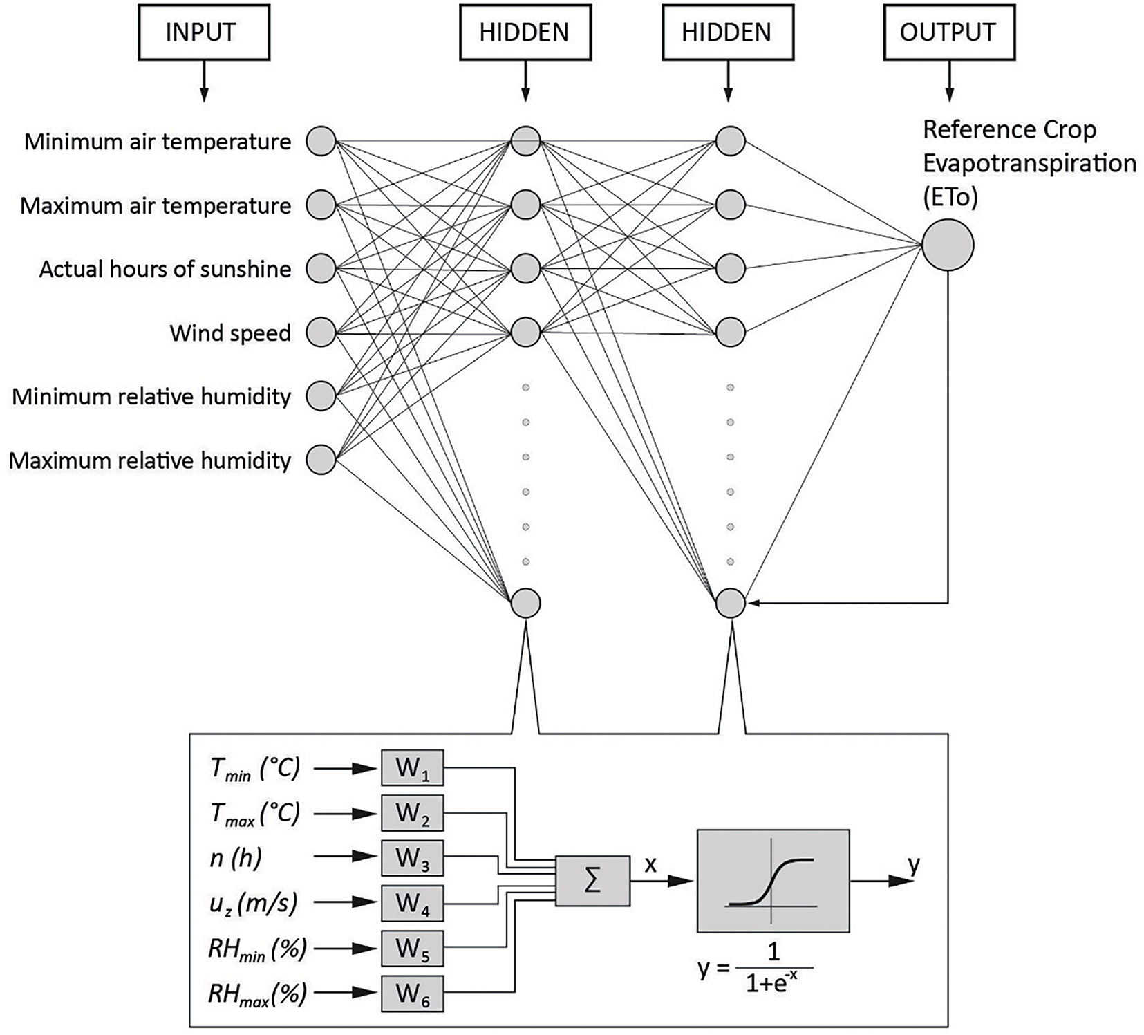
Figure 3: ANN structure of ETo with criteria and sigmoid function

In the present study, ANN analysis was done by combining the data from a total of 36 stations and using six and eight variables. After normalizing the entire dataset without separating the training and test data, the 6448 data were divided into two groups: 4340 were training data (70%), and 2018 were test data (30%). Input data with the data from six and eight variables and target data with ETo values determined using the PM method were recorded in separate tables. Thus, ANN analysis was performed using the supervised learning process. The ANN structure, similar to the others, was edited with 40 neurons and 5000 epochs using the sigmoid (log sig) activation function. The estimated output training and test results were denormalized, and the ETo prediction values were calculated as the coding progressed.

2.3 Statistical Performance Analysis

The ETo values (EToPM) calculated by the PM method were accepted as real, and the accuracy of the ETo prediction values (EToModel) obtained by the MLR and ANN models was investigated. For this, performance analyses made up of commonly used R2, Mean Absolute Error (MAE), Mean Absolute Percentage Error (MAPE), and Root Mean Squared Error (RMSE) rates were applied [20,22,24,72–74]. R2 (Eq. (4)), also known as the Coefficient of Determination in statistics, was used to find a group of sample correlations and is desired to be as close to 1 as possible [75]. The MAE is equal to the average absolute difference between the and values (Eq. (5)). MAPE is calculated as a percentage by averaging the absolute differences between the and values to the value (Eq. (6)). The RMSE is equal to the square root of the sum of the squares of the difference between the value and the value (Eq. (7)). “The estimated data agree perfectly with the reference data when RMSE is 0.” [76].

The explanations for the expressions in Eqs. (4)–(7) are as follows:

R2=1−∑i=1n(EToPM−EToModel)2∑i=1n(EToPM−EToPM¯)2(4)

MAE=1n∑i=1n|EToPM−EToModel|(5)

MAPE=[1n∑i=1n|EToPM−ETomodel|EToPM]∗100(6)

RMSE=1n∑i=1n(EToPM−EToModel)2(7)

3  Results

3.1 Application of Regression Models

For MLR analysis, after normalizing the data from each station, only the training dataset was transferred to the SPSS package program. The training dataset, which included 124 lines for 32 stations and 93 lines for four stations, was analyzed, and a mathematical model with six dependent variables was created. According to the MLR1 models in Scenario 1, 36 models for 36 stations were obtained (Appendix C). The predictive values of ETo were calculated in these models by substituting them into the normalized training and test datasets. Because the estimated ETo values ranged from 0 to 1, they were converted and denormalized. In other words, because the model was obtained with normalized values, the denormalized predictive value of ETo was found after calculating the normalized predictive value of ETo.

MLR was applied to each station’s data separately, and it was determined that the coefficients of each model differed. The coefficients of the 36 models were ranked for six variables beginning with 1 in order of absolute value from largest to smallest, and the highest numbers of the variables were marked and evaluated by summing the 1–6 point numbers. The coefficients of actual hours of sunshine (n) in 18 models and wind speed (uz) in 15 models are in the first place and have the highest values, according to the evaluation of 36 MLR1 models at the stations. Maximum air temperature (Tmax) comes in second place in 19 models and third place in 13 models. Minimum relative humidity (RHmin) came in fourth in 21 models, minimum air temperature (Tmin) came in fifth in 16 models, and maximum relative humidity (RHmax) came in sixth in 18 models. When the coefficients’ signs were examined, it was discovered that the model’s sign was positive, as the water requirements of the plants increased with air temperature (Tmax,Tmin), actual hours of sunshine (n), and wind speed (uz). Because humidity reduces the plant’s need for water, it has the opposite sign of the others and is negative (Appendix C).

When MLR was applied to all stations with six (MLR2) and eight (MLR3) variables, the first four rows in absolute value from the largest to the smallest did not change in either model. The coefficients of MLR2 and MLR3 models are uz (0.650; 0.636), Tmax (0.319; 0.339), n (0.282; 0.283) and RHmin (−0.138; −0.122), respectively. When the wind speed (uz) with the highest coefficient increases by one unit in the MLR2 model, the ETo increases by 0.650 units; when the maximum air temperature (Tmax) increases by one unit in the MLR3 model, the ETo increases by 0.339 units. The MLR2 and MLR3 models’ fifth and sixth rows alternate between RHmax and Tmin. Except for the “constant coefficient (β0; Constant),” the signs of the coefficients in the MLR2 and MLR3 models were found to be the same as those in the 36 stations, the models where the calculations were made separately. There are positive Y and negative N variables in the last two rows when the daily possible maximum daylight hours (N) and elevation (altitude) above sea level (Y) variables are added to the MLR analysis. MLR2 and MLR3 models’ R2 values are 0.965 and 0.968, respectively, and the variables adequately explain to the model because they are close to 1. The significance of F–Test is 0.000 and the models are significant since p < 0.05 (Table 3).

3.2 Application of ANN Models

ANN Analysis: For each of the 36 stations, it was performed using six variables with coding written in the Matlab program. In the coding: Firstly, the entire dataset was normalized without separating training and testing, and then 124 data for 32 stations and 93 data for four stations were analyzed as a 70% training dataset. Verification was performed using 62 data for 32 stations and 31 data for four stations, with a 30% test dataset. In the multilayer perceptron structure of ANN, it was edited with 40 neurons and 5000 epochs using the sigmoid (log sig) activation function. In the next step of the coding, the estimated output training and test results were denormalized, and the ETo prediction values were calculated.

For ANN1 model analysis, 5000 epoch iterations were completed in 10 s. The Mean Squared Error was observed to decrease towards zero at approximately 1000 epochs and to be very close to zero (2.2304 − 5) at 5000 epochs. The R value of the training data is 0.99976, which performed very well in the model description, and the R2 is 0.9995, which is very close to one (Fig. 4).

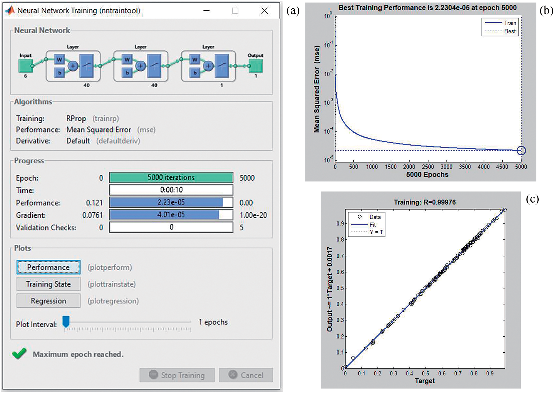
Figure 4: Training of the ANN1 model of Mersin (7) station (a), Training performence of ANN1 (b) ve error distribution of ANN1 training dataset (c)

The codes were run with six variables for the ANN2 model, and 5000 epoch iterations were done in one minute and 24 s. Likewise, iteration with eight variables in ANN3 took one minute and 25 s. The Mean Squared Error decreased towards zero at about 500 epochs and was close to zero (5.5026 − 5) after 5000 epochs, indicating that the ANN2 model performed very well. The Mean Squared Error decreased towards zero at approximately 750 epochs and was very close to zero (9.168 − 5) at 5000 epochs as a result of the ANN3 model. The R-value in the ANN2 and ANN3 models of the training data is 0.99794, 0.99656, respectively, and in the model description, R2 is 0.99588, 0.99313, indicating that the model is very close to one and well explained.

3.3 Comparison of Model Performances

MLR and ANN analyses were used to create models from the training data. Separate performance analyses of training and test data were carried out. Totally 76 models were produced which are 36 MLR1, 36 ANN1, and MLR2, ANN2, MLR3, and ANN3. MLR 1 and ANN1 were compared to each other first, and then all models were compared to each other. Finally, due to the 6448 data density, the performances of the MLR and ANN models in scenarios 1, 2, and 3 were only examined for the Mersin station.

Separate models were created with each station’s data in the MLR1 and ANN1 models, and their performances were evaluated separately. R2, MAE, MAPE, and RMSE values were examined for performance. When a total of 72 models, including MLR1 and ANN1, from 36 stations were examined, the model of R2 Çamlıyayla (18) station had the highest training data, and when combined with errors, Erdemli was the most successful station (13).

The training and test model performances of 36 models were evaluated separately. While examining the high performance of the training models, the highest values in R2 and the lowest values in errors were taken into account. It was observed that among the MLR1 models with the best performance, Alanya (4) MAE, MAPE, and RMSE values were 0.0341, 0.7790%, 0.0513, and Aladağ (24) R2 0.9946, respectively, among the ANN1 models, Çamlıyayla (18), R2 0.9997, RMSE 0.0162, and Erdemli (13) MAE, MAPE and RMSE values were 0.0105, 0.2718% and 0.0162, respectively. The best of these stations is Erdemli (13) station, which uses ANN1 model data and has a very successful performance with 0.9994 on R2. While examining the low performance of the training models, the lowest values in R2 and the highest values in errors were taken into account. Among 36 models, the error rates with the lowest performance were determined. In MLR1 models, Aydıncık (19) R2 0.9582, Ayrancı (22) MAE 0.1352, RMSE 0.1919, and Çamardı (23) MAPE 3.1262%, and in ANN1 models, Alanya (4) R2 0.7234, Mut (12) MAE 0.7143 with RMSE 0.7617, and Kızılbağ (29) MAPE 15.0142%. After the models of all stations were examined together, it was clear that MLR1 models outperform ANN1 models. MAE, RMSE, and MAPE values of Mut (12), Çamardı (23), Kızılbağ (29), and Akdere (35) stations were found to have excessive deviations in training ANN1 models (Fig. 5a).

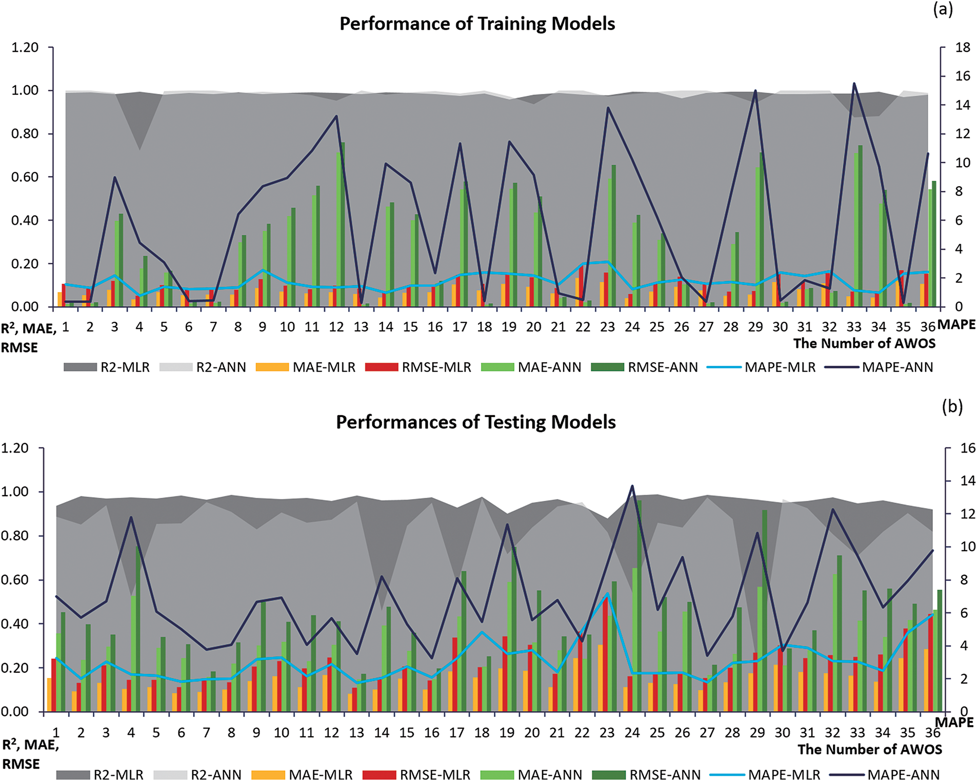
Figure 5: MLR1 and ANN1 training (a) and testing (b) performances

The performance of the testing models was also evaluated in the same way that the training models were. Çukurova (25) R2 0.9888 and Erdemli (13) MAE, MAPE, and RMSE stations with the best performance among MLR1 models had the values of 0.0831, 1.7667 percent, and 0.1091, respectively. The stations with the best performance in ANN1 models are Erdemli Tömük (27) R2 0.9743, Erdemli (13) MAE 0.1473 and RMSE 0.1729, and Karataş (16) MAPE 3.2407 percent. The best of these stations was the Erdemli (13) station, which had the data made from ANN1 model data and achieved a very successful performance of 0.9994 on R2. The Erdemli station performs well in both training and testing models. However, while ANN1 was the best in the Erdemli station’s training model, MLR1 was the best in the testing model. The low performance of the testing models was also evaluated in the same way that the training models were. Çamardı (23) is the worst-performing station in MLR1 models, with R2, MAE, MAPE, and RMSE values of 0.8789, 0.3055, 7.1726 percent, and 0.5219, respectively. Kızılbağ (29), R2 with 0.2037 is very low in ANN1 models. R2 values in Gazipaşa (14) 0.4595, Alanya (4) 0.5241, Aladağ (24) 0.5415, and Gülnar (17) 0.5774, which were close to this value, are also low. R2 values for 31 stations other than these five are above 0.70. Aladağ (24) performs the worst, with MAE, MAPE, and RMSE values of 0.6545, 13.7041 percent, and 0.9604, respectively. When the models of the entire station were examined in aggregate, it was discovered that the MLR1 models performed better in the testing models.

Furthermore, the performance of the training models outperforms the testing models. The main reason for this is that the ETo is estimated by reusing the data that was used to create the model. The MAE, RMSE, and MAPE values of Alanya (4), Aydıncık (19), Aladağ (24), Kızılbağ (29), Halkapınar İvriz (32) stations were found to have excessive deviations in the testing ANN1 models (Fig. 5b). It was observed that the columns formed by the MAE and RMSE values in the graph and the lines formed by the MAPE value continue in parallel in both MLR1 and ANN1 models (Fig. 5a,b).

EToPM value; on the graph, an example of a Mersin station was shown to compare the MLR1 and ANN1, MLR2 and ANN2, and MLR3 and ANN3 models. A similar situation was observed at the other stations as well. According to the Mersin station data analysis, while the MLR1 model coincidence with the EToPM value better in the training dataset, the model coincidence was good in the testing dataset (Fig. 6). The ANN1 model had slightly less coincidence with the EToPM than MLR1 (Fig. 6a). In other models, the opposite was the case, with ANN2 and ANN3 models coincidence better with EToPM value than MLR2 and MLR3 models. Because it was estimated using its own data, the training dataset produced better results than the testing dataset (Fig. 6b,c).

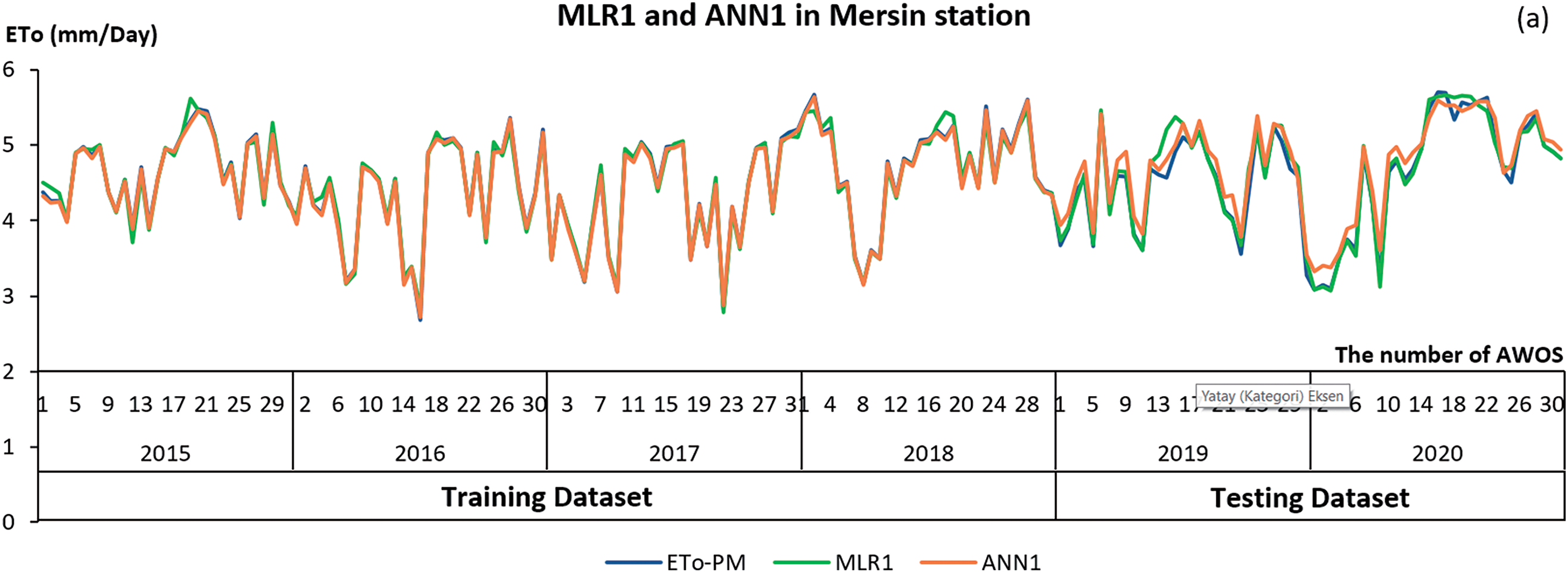
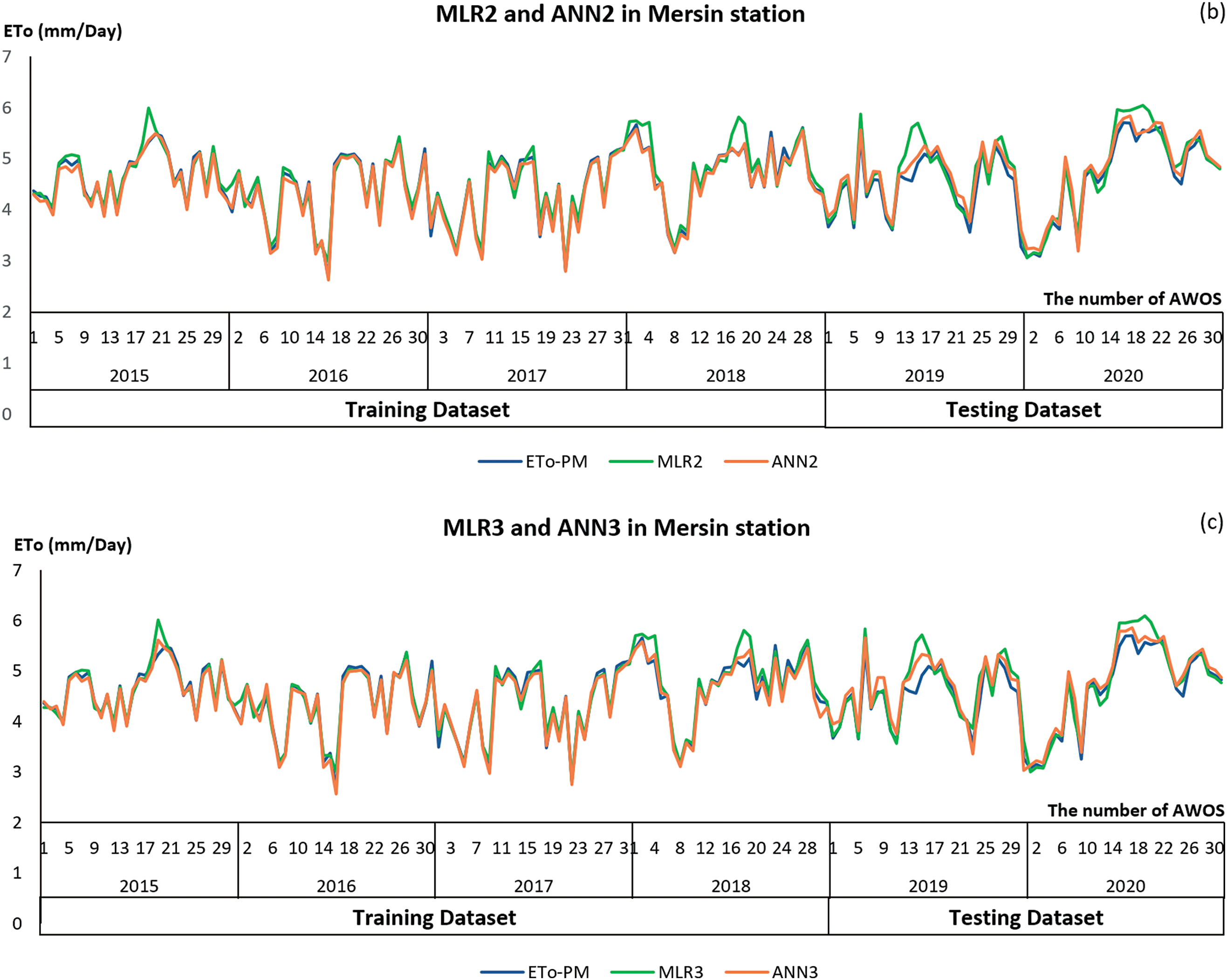
Figure 6: ETo values of Mersin station (a–c)

When the MLR2, ANN2, MLR3, and ANN3 models’ performances were compared, it was discovered that MLR1, and ANN1 performed better than the others. It was determined that MLR2, ANN2, MLR3, and ANN3 models performed better than regression models in ANN models. The ANN2 model has six variables and an R2 value of 0.9958 for the training dataset and 0.9844 for the testing dataset, making it the best model as the closest model to one. In the training dataset, the MAE, MAPE, and RMSE of the ANN2 model are 0.0678, 1.5341%, and 0.0864, respectively; in the testing dataset, 0.1387, 3.0387%, and 0.1844 were found to have less error than other models (Table 4).

The graph depicts the point distributions between the estimated ETo values obtained from the models and EToPM, as well as the line equation (Fig. 7). When the line equations were examined, it was determined that ANN is superior to MLR analysis, and the model with the closest equation to the line (y=0.9984x) in the training dataset is MLR3. The equations of the ANN2 and ANN3 models in the training dataset were found to be identical. In the regression analysis, the MLR3 model appears to perform better than the MLR2, whereas the ANN appears to perform in the opposite way. The six variables ANN2 model outperformed the eight variables ANN3 model (Fig. 7a,d).

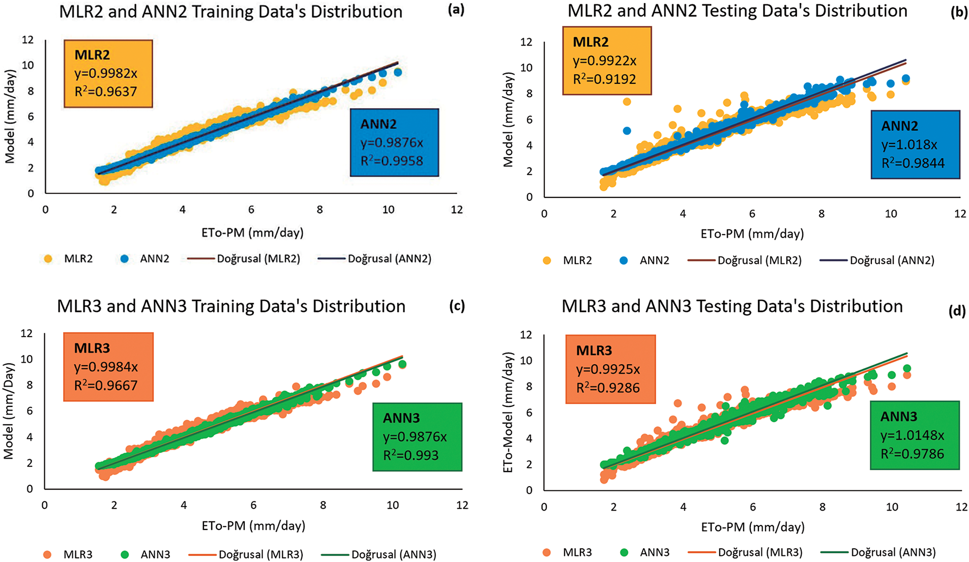
Figure 7: Distribution of model data and line equation (a–d)

4  Discussion

The present study used both empirical and statistical methods to determine the ETo value of Mersin province between May 2015 and 2020. According to the results of the collective station analysis, ANN was found to be the closest model to the EToPM values that were found by the empirical method, while MLR, one of the statistical methods, had only a good result. Unlike previous studies, this is the first for Mersin, which is located in the Mediterranean and is supported by geographic information systems, which are also among modern information systems. The values found were presented with maps.

With the collective analysis of the stations, the MLR3 model performed successfully with 0.9667, 0.1217, 2.8997%, and 0.1843 values for the training dataset and 0.9286, 0.2036, 4.2113%, and 0.3294 for the testing dataset, respectively (Table 4). In studies that performed ANN analysis for ETo estimations, the multilayer perceptron algorithm and sigmoid [51,73,77], hyperbolic tangent [19], or both [39] activation functions are commonly used. In the present study, the sigmoid function was used and solved with 5000 iterations. The collective analysis of the stations in the ANN method was found to be far more successful than the general cases of individual analyses. The stations that performed the best in terms of R2 value according to the ANN1 models in the analysis of the stations separately were Çamlıyayla (18) 0.9997 for the training dataset and Erdemli Tömük (27) 0.9743 for the testing dataset. In terms of MAE, MAPE, and RMSE values, Çamlıyayla (18) RMSE was 0.0162, and Erdemli (13) stations were 0.0105, 0.2718% for the training dataset and 0.0162, respectively, and in the testing dataset, Erdemli (13) stations MAE (0.1473) and RMSE (0.1729) and Karataş (16) stations MAPE (3.2407%) were the stations with the highest performance and the lowest error. The MAE, MAPE and RMSE of the ANN2 model were 0.0678, 1.5341%, and 0.0864 for the training dataset, 0.1387, 3.0387%, and 0.1844 for the testing dataset, respectively (Table 4). At Mersin station, the ANN2 model was very close to EToPM. When EToPM and ANN2 data distributions were examined, R2 was 0.9958 in training and 0.9844 (Table 4) in testing, and the ANN2 model performed very well in terms of both performance and visual maps (Fig. 8).

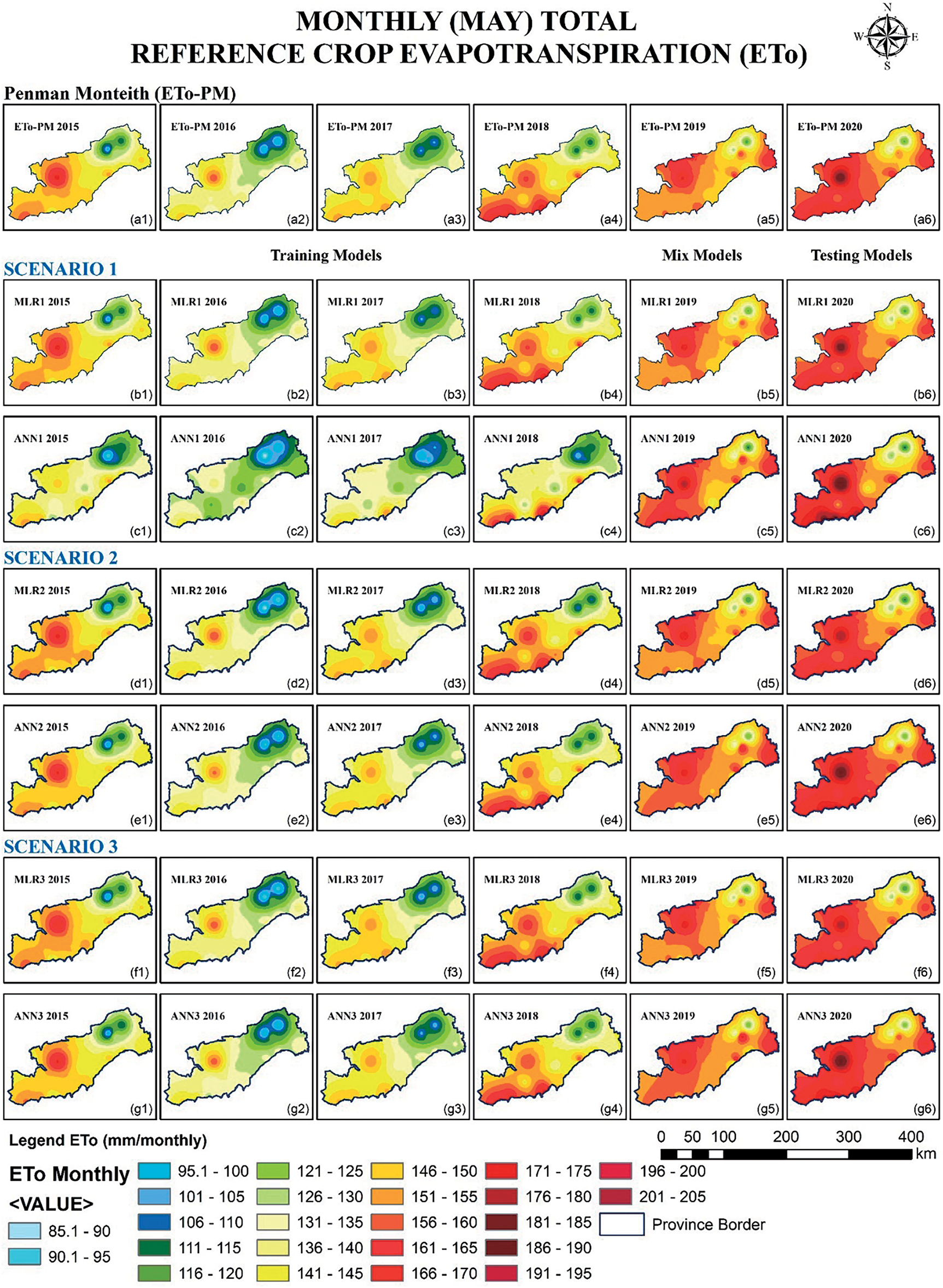
Figure 8: 2015–2020 total crop evapotranspiration for May

While ETo values were calculated and found using the PM method with ten variables, stations were analyzed using six variables in MLR and ANN analyses, and all stations were analyzed using both six and eight variables. MLR1 and ANN1 performance vary in each station. It was observed that the regression analysis performed better in the performance of the analyses performed separately for each station, whereas the ANN results performed better in the overall analysis. Because the MLR1 and ANN1 models were analyzed separately, the R2 and error rates were also analyzed separately. However, since the MLR2, ANN2, MLR3, and ANN3 models were analyzed collectively, the station errors were calculated collectively as well.

GIS is used for spatial analysis and mapping. Since it is not always possible to establish stations in or near agricultural areas, GIS plays an important role in estimating crop evapotranspiration by producing maps with the spatial distribution. Because stations are not located everywhere and the ETo value is required in every agriculturally significant location, spatial interpolation methods are essential to creating maps [78]. Kriging [79,80], Ordinary Kriging (KO) [81], Universal Kriging (KU) [82], kriging with external drift (KED) [58], and IDW [83,84] methods were used for calculating reference crop evapotranspiration (ETo) and its visualization, interpretation [85], spatial estimation, and comparison of models. In addition to these methods, interpolation was made with a spline with tension, a thin-plate spline, and a completely regularized spline [86].

In the present study, maps were created using IDW, and the total monthly ETo value was calculated using PM, MLR, and ANN methods with the assistance of GIS. The similarities and differences between PM and models were compared by examining the spatial distribution of ETo values. These maps allow for a more rapid and practical visual evaluation of the models. Furthermore, irrigation planning can be effectively conducted by estimating ETo values for locations lacking nearby meteorological stations, thus enabling better water resource management in remote or under-monitored agricultural areas. By utilizing data measurable from Automatic Weather Observation Systems (AWOS), long-term estimations can be made for irrigation planning. As AWOS data continues to be collected, more up-to-date and accurate estimations can be generated, allowing the implementation of dynamic and responsive irrigation programs. This approach supports the optimization of irrigation schedules, reduces water waste, and enhances crop productivity. The methodology and findings of this investigation serve as an invaluable guide for other researchers aiming to develop region-specific evapotranspiration models and for policymakers designing sustainable agricultural water use strategies across the country.

The station-based “MLR1 2020” (Fig. 9b) and aggregated data-based “ANN2 2020” (Fig. 9c) models, which have the best visual resemblance to the PM-ETo2020 map (Fig. 9a), were also investigated by taking into account agricultural lands that are predominantly composed of citrus orchards. It was observed that crop water consumption increased in the Tarsus (southeast) region, where agricultural lands are dense. Another district that is dense in terms of agricultural land is the Mut (Northwest) region, and it was determined that the water consumption was high (Fig. 9).

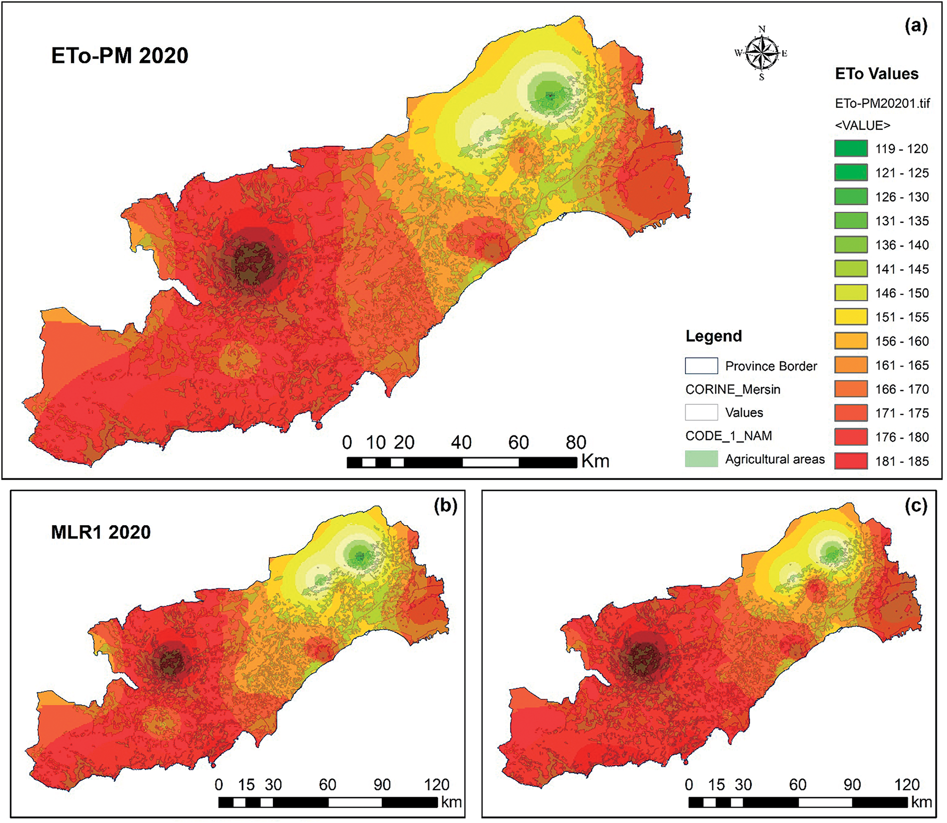
Figure 9: EToPM 2020, MLR1 2020 and ANN2 2020 Reference Crop Evapotranspiration Maps (a–c)

5  Conclusions

In the present study, the Penman-Monteith method was used to determine and map how much water the reference grass crop requires for Mersin. When the total May ETo values between 2015 and 2020 were examined, it was observed that they continued to increase year after year while the crop’s water requirement increased. The amounts of 95–119 mm/month seen in EToPM 2016 were no longer seen in EToPM 2020; on the contrary, the highest amounts, such as 170–185 mm/month, were found. The main reason for this is an increase in temperature, a decrease in humidity, and a decrease in precipitation. The significance of water and irrigation becomes increasingly obvious each year. Therefore, these maps will serve as a useful starting point for planning irrigation and drainage projects and preventing excessive water loss. Making a crop pattern map of agricultural products in Mersin is essential for determining the water consumption amounts of each crop separately.

The uniqueness of this study is that the climate data is in the form of time series, and the training data (2015–2018) and test data (2019–2020) are separated by years and analyzed separately and together in the same study. In most studies, all of the months in a year are chosen; however, in this study, only the data from May, which is one of the vegetation periods, are taken into account. With six variables, each station was analyzed separately, and MLR1 and ANN1 models were produced. MLR3 and ANN3 models were obtained with eight variables combining all station data and MLR2 and ANN2 with six variables, and variables added. Among these, the ANN2 model combined with the MLR1 model at Erdemli (13) station had the best performance with its R2, MAE, MAPE, and RMSE values.

Raw files of climate data will be examined and read directly in the Python programming language in future studies. Actual hours of sunshine (N) and extraterrestrial radiation (Ra) data will be determined by calculating the latitude information of the stations rather than obtaining the data from the relevant tables. It is aimed to determine the water consumption of the most common locally grown crops (lemon, olive, strawberry, banana, peach, carob, etc.) and associate them with the map, as well as present them interactively on the internet by providing a link during the map production phase, based on the ETo values estimated from climate data. A deep learning technique, a sophisticated subset of Artificial Neural Networks (ANN), will be utilized to determine the model that most accurately represents real-world situations. Experimental studies will be performed utilizing diverse data combinations, including meteorological variables like precipitation and air pressure.

Acknowledgement: This study was performed within the scope of the “Research Protocol” of Mersin University, Engineering Faculty, Department of Geomatics Engineering, Mersin Provincial Directorate of Meteorology Department, Governorship of Mersin and Turkish State Meteorological Service.

Funding Statement: The authors received no specific funding for this study.

Author Contributions: The authors confirm contribution to the paper as follows: Fatma Bunyan Unel, the research management: writing—original draft preparation, investigation, analysis and visualization; Lutifiye Kusak: investigation, supervision, editing and validation; Murat Yakar, Abdullah Sahin, Hakan Dogan and Fikret Demir: writing—review and editing. All authors reviewed the results and approved the final version of the manuscript.

Availability of Data and Materials: Due to the nature of this research, participants of this study did not agree for their data to be shared publicly, so supporting data is not available.

Ethics Approval: Not applicable.

Conflicts of Interest: The authors declare no conflicts of interest to report regarding the present study.

Symbols

Appendix A

Appendix B

Appendix C

References

1. Lazzara P, Rana G. The crop coefficient (Kc) values of the major crops grown under Mediterranean climate. Ital J Agrometeorol. 2010;15:25–40. [Google Scholar]

2. Usta S, Gençoğlan S, Gençoğlan C. Establishing the flow charts that can be used in the design of irrigation automation systems. Turkish J Agric—Food Sci Technol. 2019;7(7):1014–20. [Google Scholar]

3. WMO. Guide to instruments and methods of observation. Geneva, Switzerland: World Meteorological Organization; 2018. [Google Scholar]

4. Karaca C, Büyüktaş D, Bastug R, Aydınşakir K, Tekelioğlu B. Antalya koşullarında kıyas bitki su tüketiminin alansal ve zamansal dağılımının belirlenmesi. Derim. 2017;34(2)158–171. (In Turkish). doi:10.16882/derim.2017.292134. [Google Scholar] [CrossRef]

5. Mousumi KA, Mojid A, Ahmad T, Uddin Z, Parvez MF. Climate-induced historical drift of reference evapotranspiration in Mymensingh region of Bangladesh. J Bangladesh Agric Univ. 2019;17(2):258–64. [Google Scholar]

6. Bayramoğlu E. Trabzon İlinde İklim Değişikliğinin Mevsimsel Bitki Su Tüketimine Etkisi : penman-Monteith Yöntemi. Kastamonu Üniversitesi. Orman Fakültesi Dergisi. 2013;13(2):300–6. (In Turkish). [Google Scholar]

7. Gürgülü H, Ul MA. İzmir’de Yetiştirilen Bazı Bitkiler İçin Bitki Su Tüketimi Değerleri ve Sulama Programları. J Agric Faculty of Ege University. 2017;54:311–7. (In Turkish). [Google Scholar]

8. Allen RG, Pereira LS, Raes D, Smith M, Ab W. Crop evapotranspiration—guidelines for computing crop water requirements—FAO Irrigation and drainage paper 56. Rome, Italy: FAO—Food and Agriculture Organization of the United Nations; 1998. [Google Scholar]

9. Sattari MT, Apaydin H, Shamshirband S. Performance evaluation of deep learning-based gated recurrent units (GRUs) and tree-based models for estimating ETo by using limited meteorological variables. Mathematics. 2020;8(6):972. doi:10.3390/MATH8060972. [Google Scholar] [CrossRef]

10. Salam R, Reza A, Islam T. Potential of RT, bagging and RS ensemble learning algorithms for reference evapotranspiration prediction using climatic data-limited humid region in Bangladesh. J Hydrol. 2020;590(12):125241. doi:10.1016/j.jhydrol.2020.125241. [Google Scholar] [CrossRef]

11. Gonzalez RT, Subathra MSP, Manoj N, Verrastro S, George ST. Modelling the daily reference evapotranspiration in semi-arid region of South India : a case study comparing ANFIS and empirical models. Inf Process Agric. 2021;8(1):173–84. doi:10.1016/j.inpa.2020.02.003. [Google Scholar] [CrossRef]

12. Jothiprakash KRV. Multi-output ANN model for prediction of seven meteorological parameters in a weather station. J Inst Eng (India) Ser A. 2014;95(4):221–9. doi:10.1007/s40030-014-0092-9. [Google Scholar] [CrossRef]

13. Dias SHB, Filgueiras R, Filho EIF, Arcanjo GS, Da Silva GH, Mantovani EC, et al. Reference evapotranspiration of Brazil modeled with machine learning techniques and remote sensing. PLoS One. 2021;16(2):e0245834. doi:10.1371/journal.pone.0245834. [Google Scholar] [PubMed] [CrossRef]

14. Ng JL, Huang YF, Yong SLS, Tan JW. Comparative assessment of reference crop evapotranspiration models and its sensitivity to meteorological variables in Peninsular Malaysia. Stoch Environ Res Risk Assess. 2022;36:3557–75. [Google Scholar]

15. Yadeta D, Kebede A, Tessema N. Potential evapotranspiration models evaluation, modelling, and projection under climate scenarios, Kesem sub-basin, Awash River basin. Ethiopia Model Earth Syst Environ. 2020;6(4):2165–76. doi:10.1007/s40808-020-00831-9. [Google Scholar] [CrossRef]

16. Yirga SA. Modelling reference evapotranspiration for Megecha catchment by multiple linear regression intergovernmental panel on climate change. Model Earth Syst Environ. 2019;5(3):471–7. doi:10.1007/s40808-019-00574-2. [Google Scholar] [CrossRef]

17. Diez FJ, Navas-Gracia LM, Chico-Santamarta L, Correa-Guimaraes A, Martínez-Rodríguez A. Prediction of horizontal daily global solar irradiation using artificial neural networks (ANNs) in the Castile and León region. Spain Agronomy. 2020;10(1):96. doi:10.3390/agronomy10010096. [Google Scholar] [CrossRef]

18. Mehdizadeh S. Estimation of daily reference evapotranspiration (ETo) using artificial intelligence methods: offering a new approach for lagged ETo data-based modeling. J Hydrol. 2018;559(1–2):794–812. doi:10.1016/j.jhydrol.2018.02.060. [Google Scholar] [CrossRef]

19. Ferreira LB, da Cunha FF. New approach to estimate daily reference evapotranspiration based on hourly temperature and relative humidity using machine learning and deep learning. Agric Water Manag. 2020;234:106113. doi:10.1016/j.agwat.2020.106113. [Google Scholar] [CrossRef]

20. Saggi MK, Jain S. Reference evapotranspiration estimation and modeling of the Punjab Northern India using deep learning. Comput Electron Agric. 2019;156(9):387–98. doi:10.1016/j.compag.2018.11.031. [Google Scholar] [CrossRef]

21. Valle LCG, Ventura TM, Gomes RSR, Nogueira JDS, Lobo FDA, Vourlitis GL, et al. Comparative assessment of modelled and empirical reference evapotranspiration methods for a brazilian savanna. Agric Water Manag. 2020;232(80):106040. doi:10.1016/j.agwat.2020.106040. [Google Scholar] [CrossRef]

22. Wu L, Peng Y, Fan J, Wang Y, Huang G. A novel kernel extreme learning machine model coupled with K-means clustering and firefly algorithm for estimating monthly reference evapotranspiration in parallel computation. Agric Water Manag. 2021;245(2):106624. doi:10.1016/j.agwat.2020.106624. [Google Scholar] [CrossRef]

23. Gocić M, Motamedi S, Shamshirband S, Petkovic D, Ch S, Hashim R, et al. Soft computing approaches for forecasting reference evapotranspiration. Comput Electron Agric. 2015;113(1):164–73. doi:10.1016/j.compag.2015.02.010. [Google Scholar] [CrossRef]

24. Kisi O. Pan evaporation modeling using least square support vector machine, multivariate adaptive regression splines and M5 model tree. J Hydrol. 2015;528(12):312–20. doi:10.1016/j.jhydrol.2015.06.052. [Google Scholar] [CrossRef]

25. Aghelpour P, Norooz-Valashedi R. Predicting daily reference evapotranspiration rates in a humid region, comparison of seven various data-based predictor models. Stoch Environ Res Risk Assess. 2022;36(12):4133–55. doi:10.1007/s00477-022-02249-4. [Google Scholar] [CrossRef]

26. Petković B, Petković D, Kuzman B, Milovančević M, Wakil K, Ho LS, et al. Neuro-fuzzy estimation of reference crop evapotranspiration by neuro fuzzy logic based on weather conditions. Comput Electron Agric. 2020;173(3):105358. doi:10.1016/j.compag.2020.105358. [Google Scholar] [CrossRef]

27. Sanikhani H, Kisi O, Maroufpoor E, Yaseen ZM. Temperature-based modeling of reference evapotranspiration using several artificial intelligence models: application of different modeling scenarios. Theor Appl Climatol. 2019;135(1–2):449–62. doi:10.1007/s00704-018-2390-z. [Google Scholar] [CrossRef]

28. Tabari H, Kisi O, Ezani A, Talaee PH. SVM, ANFIS, regression and climate based models for reference evapotranspiration modeling using limited climatic data in a semi-arid highland environment. J Hydrol. 2012;444-445(7):78–89. doi:10.1016/j.jhydrol.2012.04.007. [Google Scholar] [CrossRef]

29. Tao H, Diop L, Bodian A, Djaman K, Ndiaye PM, Yaseen ZM. Reference evapotranspiration prediction using hybridized fuzzy model with firefly algorithm: regional case study in Burkina Faso. Agric Water Manag. 2018;208(2):140–51. doi:10.1016/j.agwat.2018.06.018. [Google Scholar] [CrossRef]

30. Feng Y, Peng Y, Cui N, Gong D, Zhang K. Modeling reference evapotranspiration using extreme learning machine and generalized regression neural network only with temperature data. Comput Electron Agric. 2017;136(1):71–8. doi:10.1016/j.compag.2017.01.027. [Google Scholar] [CrossRef]

31. Ruiming F, Shijie S. Daily reference evapotranspiration prediction of Tieguanyin tea plants based on mathematical morphology clustering and improved generalized regression neural network. Agric Water Manag. 2020;236(1):106177. doi:10.1016/j.agwat.2020.106177. [Google Scholar] [CrossRef]

32. Ahmed AAM, Deo RC, Feng Q, Ghahramani A, Raj N, Yin Z, et al. Hybrid deep learning method for a week-ahead evapotranspiration forecasting. Stoch Environ Res Risk Assess. 2022;36:831–49. [Google Scholar]

33. Tejada ATJr., Ella VB, Lampayan RM, Reaño CE. Modeling reference crop evapotranspiration using support vector machine (SVM) and extreme learning machine (ELM) in region IV-A, Philippines. Water. 2022;14(5):754. doi:10.3390/w14050754. [Google Scholar] [CrossRef]

34. Wu Z, Chen X, Cui N, Zhu B, Gong D, Han L, et al. Optimized empirical model based on whale optimization algorithm for simulate daily reference crop evapotranspiration in different climatic regions of China. J Hydrol. 2022;612(128084):1–17. doi:10.1016/j.jhydrol.2022.128084. [Google Scholar] [CrossRef]

35. Afzaal H, Farooque AA, Abbas F, Acharya B, Esau T. Computation of evapotranspiration with artificial intelligence for precision water resource management. Appl Sci. 2020;10(5):1621. doi:10.3390/app10051621. [Google Scholar] [CrossRef]

36. Dong J, Xing L, Cui N, Zhao L, Guo L, Wang Z, et al. Estimating reference crop evapotranspiration using improved convolutional bidirectional long short-term memory network by multi-head attention mechanism in the four climatic zones of China. Agric Water Manag. 2024;292:108665. doi:10.1016/j.agwat.2023.108665. [Google Scholar] [CrossRef]

37. Baishnab U, Hossen Sajib MS, Islam A, Akter S, Hasan A, Roy T, et al. Deep learning approaches for short-crop reference evapotranspiration estimation: a case study in Southeastern Australia. Earth Sci Inform. 2025;18:4. doi:10.1007/s12145-024-01616-9. [Google Scholar] [CrossRef]

38. Zhang J, Ding Y, Zhu L, Wan Y, Chai M, Ding P. Estimating and forecasting daily reference crop evapotranspiration in China with temperature-driven deep learning models. Agric Water Manag. 2025;307:109268. doi:10.1016/j.agwat.2024.109268. [Google Scholar] [CrossRef]

39. Genaidy MA. Estimating of evapotranspiration using artificial neural network. Misr J Agric Eng. 2020;37(1):81–94. doi:10.21608/mjae.2020.94971. [Google Scholar] [CrossRef]

40. Gao Z, Yang D, Li B, Gao Z, Li C. Reference crop evapotranspiration prediction based on gated recurrent unit with quantum inspired multi-head self-attention mechanism. Water Resour Manag. 2025;39(3):1481–1501. doi:10.1007/s11269-024-04016-2. [Google Scholar] [CrossRef]

41. Elbeltagi A, Kumar N, Chandel A, Arshad A, Pande CB, Islam ARMT. Modelling the reference crop evapotranspiration in the Beas-Sutlej basin (Indiaan artificial neural network approach based on different combinations of meteorological data. Environ Monit Assess. 2022;194(3):141. doi:10.1007/s10661-022-09812-0. [Google Scholar] [PubMed] [CrossRef]

42. Manikumari N, Vinodhini G, Murugappan A. Modelling of reference evapotransipration using climatic parameters for irrigation scheduling using machine learning. ISH J Hydraul Eng. 2020;28(sup1):272–81. doi:10.1080/09715010.2020.1771783. [Google Scholar] [CrossRef]

43. de Oliveira e Lucas P, Alves MA, de Lima e Silva PC, Guimarães FG. Reference evapotranspiration time series forecasting with ensemble of convolutional neural networks. Comput Electron Agric. 2020;177(6):105700. doi:10.1016/j.compag.2020.105700. [Google Scholar] [CrossRef]

44. Fernández-López A, Marín-Sánchez D, García-Mateos G, Ruiz-Canales A, Ferrández-Villena-García M, Molina-Martínez JM. A machine learning method to estimate reference evapotranspiration using soil moisture sensors. Appl Sci. 2020;10(6):1912. doi:10.3390/app10061912. [Google Scholar] [CrossRef]

45. Zhang Y, Zhao Z, Zheng J. CatBoost : a new approach for estimating daily reference crop evapotranspiration in arid and semi-arid regions of Northern China. J Hydrol. 2020;588(1):125087. doi:10.1016/j.jhydrol.2020.125087. [Google Scholar] [CrossRef]

46. Zhou H, Ma L, Xiang Y, Su Y, Li J, Chen J, et al. Estimating reference evapotranspiration using hybrid models optimized by bio-inspired algorithms combined with key meteorological factors. Comput Electron Agric. 2025;230(3):109862. doi:10.1016/j.compag.2024.109862. [Google Scholar] [CrossRef]

47. Yong SLS, Ng JL, Huang YF, Ang CK. Estimation of reference crop evapotranspiration with three different machine learning models and limited meteorological variables. Agronomy. 2023;13(4):1048. doi:10.3390/agronomy13041048. [Google Scholar] [CrossRef]

48. Dong J, Xing L, Cui N, Guo L, Liang C, Zhao L, et al. Estimating reference crop evapotranspiration using optimized empirical methods with a novel improved Grey Wolf Algorithm in four climatic regions of China. Agric Water Manag. 2024;291(2):108620. doi:10.1016/j.agwat.2023.108620. [Google Scholar] [CrossRef]

49. Rana Ikram RMA, Mostafa RR, Chen Z, Islam ARMT, Kisi O, Kuriqi A, et al. Advanced hybrid metaheuristic machine learning models application for reference crop evapotranspiration prediction. Agronomy. 2023;13(1):98. doi:10.3390/agronomy13010098. [Google Scholar] [CrossRef]

50. Zhao L, Zhao X, Pan X, Shi Y, Qiu Z, Li X, et al. Prediction of daily reference crop evapotranspiration in different Chinese climate zones: combined application of key meteorological factors and Elman algorithm. J Hydrol. 2022;610(3):127822. doi:10.1016/j.jhydrol.2022.127822. [Google Scholar] [CrossRef]

51. Tikhamarine Y, Malik A, Souag-Gamane D, Kisi O. Artificial intelligence models versus empirical equations for modeling monthly reference evapotranspiration. Environ Sci Pollut Res Int. 2020 Aug;27(24):30001–19. [Google Scholar]

52. Adnan RM, Chen Z, Yuan X, Kisi O, El-Shafie A, Kuriqi A, et al. Reference evapotranspiration modeling using new heuristic methods. Entropy. 2020;22(5):547. doi:10.3390/e22050547. [Google Scholar] [PubMed] [CrossRef]

53. DHA. Mersin Tarsus Şelalesinin Görüntüsü. News; 2021. (In Turkish). [cited 2025 May 21]. Available from: https://www.milliyet.com.tr/yerel-haberler/mersin/tarsus/tarsus-selalesinin-goruntusu-ziyaretcileri-uzdu-6526879. [Google Scholar]

54. SGB. Tarım Ürünleri Piyasaları Raporu, Limon, T.C. Tarım ve Orman Bakanlığı, Tarımsal Ekonomi ve Politika Geliştirme Enstitüsü (TEPGE). 2020. (In Turkish) [cited 2025 May 21]. Available from: https://arastirma.tarimorman.gov.tr/tepge/Belgeler/PDF%20Tar%C4%B1m%20%C3%9Cr%C3%BCnleri%20Piyasalar%C4%B1/2020-Temmuz%20Tar%C4%B1m%20%C3%9Cr%C3%BCnleri%20Raporu/Limon,%20Temmuz-2020,%20Tar%C4%B1m%20%C3%9Cr%C3%BCnleri%20Piyasa%20Raporu.pdf. [Google Scholar]

55. IBM SPSS Statistics. Unlock more than 150 statistical procedures. [Internet]. [cited 2025 May 17]; 2025. Available from: https://www.ibm.com/products/spss-statistics. [Google Scholar]

56. Matlab Designed for the way you think and the work you do. Mathworks. [Internet]. [cited 2025 May 17]. Available from: https://www.mathworks.com/products/matlab.html. [Google Scholar]

57. The ASCE sandardized reference evapotranspiration equation. Reston, VA: USA: ASCE; 2005. doi:10.1061/9780784408056. [Google Scholar] [CrossRef]

58. Čadro S, Cherni-Čadro S, Marković M, Žurovec J. A reference evapotranspiration map for Bosnia and Herzegovina. Int Soil Water Conserv Res. 2019;7(1):89–101. doi:10.1016/j.iswcr.2018.11.002. [Google Scholar] [CrossRef]

59. Şarlak N, Bağçaci SÇ. The assesment of empirical potential evapotranspiration methods: a case study of Konya closed basin. Tek Dergi. 2020;31(1):9755–72. doi:10.18400/TEKDERG.408019. [Google Scholar] [CrossRef]

60. Sykes AO. An introduction to regression analysis. Chicago, IL, USA: Coase-Sandor Institute for Law & Economics Working Paper; 1993. [Google Scholar]

61. Seber GAF, Lee AJ. Linear regression analysis. 2nd ed. Hoboken, NJ, USA: John Wiley & Sons Publication; 2003. [Google Scholar]

62. Draper NR, Smith H. Applied regression analysis. 3rd ed. Montreal, QC, Canada: John Wiley & Sons, Inc.; 1998. [Google Scholar]

63. Dalgaard P. Introductory Statistics with R. 2nd ed. Berlin, Germany: Springer Science+Business Media, LLC; 2008. [Google Scholar]

64. Altunışık R, Coşkun R, Bayraktaroğlu S, Yıldırım E. Sosyal Bilimlerde Araştırma Yöntemleri: SPSS Uygulamalı. 6th ed. Sakarya, Turkey: Sakarya Yayıncılık; 2010. (In Turkish). [Google Scholar]

65. Aggarwal CC. Data mining. Cham, Switzerland: Springer International Publishing; 2015. [Google Scholar]

66. Lin CC, Mohan SB. Effectiveness comparison of the residential property mass appraisal methodologies in the USA. Int J Hous Mark Anal. 2011;4(3):224–43. doi:10.1108/17538271111153013. [Google Scholar] [CrossRef]

67. Shanmuganathan S, Samarasinghe S. Artificial neural network modelling, studies in computational intelligence. Cham, Switzerland: Springer International Publishing; 2016. [Google Scholar]

68. Haykin S. Neural networks: a comprehensive foundation. 2nd ed. London, UK: Pearson Education; 1999. [Google Scholar]

69. Haykin S. Neural networks and learning machines. 3rd ed. London, UK: Pearson Education; 2009. [Google Scholar]

70. Beale MH, Hagan MT, Demuth HB. Neural network ToolboxTM 7 user’s guide. Natick, MA, USA: MatLAB the MathWorks; 2010. [Google Scholar]

71. Elbeltagi A, Nagy A, Mohammed S, Pande CB, Kumar M, Bhat SA, et al. Combination of limited meteorological data for predicting reference crop evapotranspiration using artificial neural network method. Agronomy. 2022;12(2):516. doi:10.3390/agronomy12020516. [Google Scholar] [CrossRef]

72. Fan J, Ma X, Wu L, Zhang F, Yu X, Zeng W. Light gradient boosting machine : an efficient soft computing model for estimating daily reference evapotranspiration with local and external meteorological data. Agric Water Manag. 2019;225(9):105758. doi:10.1016/j.agwat.2019.105758. [Google Scholar] [CrossRef]

73. Gocić M, Petković D, Shamshirband S, Kamsin A. Comparative analysis of reference evapotranspiration equations modelling by extreme learning machine. Comput Electron Agric. 2016;127(3):56–63. doi:10.1016/j.compag.2016.05.017. [Google Scholar] [CrossRef]

74. Wu L, Fan J. Comparison of neuron-based, kernel-based, tree-based and curvebased machine learning models for predicting daily reference evapotranspiration. PLoS One. 2019;14(5):e0217520. doi:10.1371/journal.pone.0217520. [Google Scholar] [PubMed] [CrossRef]

75. Heiberger RM, Holland B. Statistical analysis and data display: an intermediate course with examples in R. 2nd ed. New York, NY, USA: Springer Science+Business Media; 2015. [Google Scholar]

76. Awal R, Habibi H, Fares A, Deb S. Estimating reference crop evapotranspiration under limited climate data in West Texas. J Hydrol Reg Stud. 2020;28(4):100677. doi:10.1016/j.ejrh.2020.100677. [Google Scholar] [CrossRef]

77. Alves WB, Rolim GDS, Aparecido LEDO. Reference evapotranspiration forecasting by artificial neural networks. Eng Agric. 2017;37(6):1116–25. doi:10.1590/1809-4430-eng.agric.v37n6p1116-1125/2017. [Google Scholar] [CrossRef]

78. Santos JEO, da Cunha FF, Filgueiras R, da Silva GH, Teixeira AHDC, Silva FCDS, et al. Performance of SAFER evapotranspiration using missing meteorological data. Agric Water Manag. 2020;233(1):106076. doi:10.1016/j.agwat.2020.106076. [Google Scholar] [CrossRef]

79. Tomas-Burguera M, Vicente-Serrano SM, Beguería S, Reig F, Latorre B. Reference crop evapotranspiration database in Spain (1961–2014). Earth Syst Sci Data. 2019;11(4):1917–30. doi:10.5194/essd-11-1917-2019. [Google Scholar] [CrossRef]

80. Unel FB, Kusak L, Yakar M, Sahin A, Doğan H, Demir F. Geostatistical mapping of reference crop evapotranspiration (ETo). In: 2nd Intercontinental Geoinformation Days (IGD); 2021 May 5–6; Mersin, Turkey. p. 60–63. [Google Scholar]

81. Júnior JCDS, Medeiros V, Garrozi C, Montenegro A, Gonçalves GE. Random forest techniques for spatial interpolation of evapotranspiration data from Brazilian’s Northeast. Comput Electron Agric. 2019;166:105017. doi:10.1016/j.compag.2019.105017. [Google Scholar] [CrossRef]

82. Borges MIS, Diaz NMM. Comparative assessment and spatial prediction of the reference evapotranspiration through geostatistical methods. Bioagro. 2020;32(2):107–16. [Google Scholar]

83. Hodam S, Sarkar S, Marak AGR. Spatial interpolation of reference evapotranspiration in India : comparison of IDW and Kriging Methods. J Inst Eng Ser A. 2017;98(2):511–24. doi:10.1007/s40030-017-0241-z. [Google Scholar] [CrossRef]

84. Okechukwu ME, Mbajiorgu CC. Spatial distribution of rainfall and reference evapotranspiration in southeast Nigeria. Agric Eng Int: CIGR J. 2020;22(1):1–8. [Google Scholar]

85. Kiefer MT, Andresen JA, Doubler D, Pollyea A. Development of a gridded reference evapotranspiration dataset for the Great Lakes region. J Hydrol Reg Stud. 2019;24:100606. doi:10.1016/j.ejrh.2019.100606. [Google Scholar] [CrossRef]

86. Güler M. A comparison of different interpolation methods using the geographical information system for the production of reference evapotranspiration maps in Turkey. J Meteorol Soc Japan. 2014;92(3):227–40. doi:10.2151/jmsj.2014-303. [Google Scholar] [CrossRef]