Seabed Classification from Multi-Frequency Multibeam Data: A Study from Selorejo, Malang, Indonesia

1  Introduction

Effective management of the natural resources requires a comprehensive understanding of the resource’s extent, geographical distribution, and ecological characteristics. Maps serve as the primary tool for recording and disseminating this information. It is possible to accurately assess the compatibilities and conflicts between human usage and the environment, by combining these maps with spatial information on human activities and to implement effective management strategies to mitigate any impacts [1]. High-precision habitat mapping is essential for identifying and quantifying the effects of human activity on the seafloor. Seabed sediment classification, as a representative of seafloor ecosystems, is crucial for marine geological study, marine environment monitoring, marine engineering construction, and seabed biotic and abiotic resource assessment [2]. Seabed classification is the process of categorizing and describing the various types of seafloor or ocean floor substrates based on their geological, biological, and physical characteristics.

Seabed classification, often referred to as seafloor classification or benthic classification, involves the categorization and characterization of the composition, texture, and features of the underwater topography or seabed found at the bottom of oceans, seas, lakes, or rivers. Seabed categorization is a crucial tool for understanding the characteristics of the ocean floor and determining its suitability for various applications. The process of seabed classification generally encompasses the following aspects (e.g., seabed features and composition, geological, and geomorphological classification). The composition refers to the specific components that compose the seafloor. The composition of sediment in an area can encompass various forms, including sand, silt, clay, gravel, or mud, along with rocks, coral reefs, or biological substances. Understanding the composition is essential for conducting environmental assessments and habitat studies. The seabed texture is determined by the size and arrangement of particles or features found on the seafloor. It aids in assessing whether the texture, is rough, coarse, or fine, of the sediment or substrate [3].

Acoustic remote sensing is an effective method for classifying seabed sediment because it has a large coverage range and is less expensive than collecting seafloor samples [4]. The acoustic-based indirect techniques are advantageous due to their great coverage, dense sampling, high efficiency, and low cost, which makes them commonly employed for seabed sediment categorization [5]. The acoustic seabed classification has been widely used and recognized as a valuable tool. This classification is essential for a range of scientific, industrial, and environmental applications, such as marine resource management, habitat mapping, navigation, and offshore infrastructure development. Creating continuous surfaces of projected species of sediment distributions and categorical maps of geomorphic features and biotopes are the goals of the seabed classification process, which also forecasting biota and substrate distributions across large spatial scales. These maps are crucial for marine spatial planning, risk assessments of hazards, assessments of fisheries resources, and marine biodiversity assessments [6]. The advancement of hydroacoustic technology has led to the development of various underwater surveying equipment, including single beam systems, multibeam systems, and side scan sonar [4].

Multibeam echosounders (MBES) have emerged as the preferred instrument for studying and mapping the maritime environment [7]. The MBES operates by emitting acoustic waves and capturing the echo of the sound with a transducer to detect the presence of underwater objects [8]. Most multibeam systems operate around a single frequency or within a narrow band around the central frequency (monochromatic), and the possibility of comparable reactions from different soil types made it difficult to analyse and classify by backscatter data [1,9]. Consequently, it is necessary to run the exact same line repeatedly in order to acquire backscatter at multiple frequencies, resulting in ineffective and complex data collection [10]. However, due to technological advancements, the multispectral multibeam system are able to modify the frequency on a ping-by-ping basis, allowing for multi-spectral acoustic measurements with a single pass over the survey area [1].

This study aims to produce sediment maps by implementing multi-frequency multibeam data using a machine learning algorithm approach. The study’s objectives are as follows: (1) Produce backscatter mosaic derived from multiple frequency backscatter data; (2) Generate sediment maps using supervised classification machine learning algorithms; and (3) Assess the accuracy of classified maps derived from multi-frequency data.

2  Method

2.1 Study Area

The study area, located in Waduk Selorejo, encompasses a total area of 158,874 square meters (Fig. 1). A popular tourist attraction, Waduk Selorejo is in Pandansari Village, Ngantang District, Malang Regency, East Java. The state-owned company Perum Jasa Tirta oversees managing water resources, and it is also in charge of the reservoir. It is important to note that the formation of the Selorejo Reservoir involved obstructing the courses of several rivers, including the Kali Konto, Lahar Kletak, Kali Kwayangan, and numerous smaller ones. Because of this special quality, Waduk Selorejo offers a beautiful and serene atmosphere that attracts both locals and visitors. The reservoir is a great place for a variety of research projects, such as sediment mapping and environmental monitoring, because of its beautiful surroundings and abundant wildlife.

Figure 1: The study was located at part of Waduk Selorejo, Pandansari Village, Ngantang District, Malang Regency, East Java

2.2 Bathymetry and Backscatter Data

An MBES data acquisition procedure entails a number of phases in order to gather high-resolution bathymetric and backscatter seabed data. Before collecting data, survey planning must be completed by selecting the survey area while considering the goals of the project, the depth range, the surrounding conditions, and any noteworthy features. Subsequently, a NORBIT iWBMS model from Norbit MBES (NORBIT Subsea) (Trondheim, Norway) with a built-in Sound Velocity Probe (SVP) is used for this survey (Fig. 2). This survey was conducted from 2 July until 6 July at Waduk Selorejo, Desa Pandansari, Kecamatan Ngantang, Kabupaten Malang, Jawa Timur, Indonesia. This MBES system is only capable of operating with a single frequency (e.g., 200, 400, 550, or 700 kHz). In the study area of this research, multi-frequency (e.g., 200, 400, 550, and 700 kHz) data were collected. A hydrography software (Hypack 2018) is used for MBES data collection.

Figure 2: Multibeam echosounder system used in this study (NORBIT iWBMS MBES)

2.3 Ground Truth Data

In the absence of actual ground truth data, this study employed a random sampling technique to extract representative samples from the Angular Range Analysis (ARA) characterization [11] across four different frequencies. A total of 26 samples were selected based on their distinct backscatter responses observed in the FMGT 7.8.4 software by QPS. These samples were treated as pseudo ground truth data and were manually labeled according to their backscatter characteristics, such as intensity patterns that typically represent gravel, coarse sand, or sandy gravel. The relative spatial distribution of the samples is illustrated in Fig. 3; however, exact geographic coordinates were not recorded, hence the locations are referred to as relative rather than absolute. This approach was necessary due to the unavailability of verified seabed sediment data. Despite this limitation, the sampling was performed carefully to ensure coverage of diverse backscatter patterns, providing meaningful input for machine learning classification. 75% of these samples were used to train the algorithm, while the remaining 25% were reserved for model validation. The resolution of the backscatter mosaic used (0.5 m) enhances the granularity of feature detection, and the selection of training data at this resolution aims to reflect the detailed textural variation captured in the mosaic. While the approach does not replace real ground-truthing, it offers a practical alternative for preliminary sediment classification and model training using multi-frequency multibeam data.

Figure 3: Process of selecting sample on ARA characterisation for ground truthing

2.4 Data Processing

In MBES surveys, data processing involves a comprehensive workflow that includes both preprocessing and postprocessing steps to transform raw data into reliable and usable information. Preprocessing lays the foundation for subsequent processing by cleaning, correcting, and enhancing raw MBES data to ensure its quality and reliability. This phase entails removing noise, calibrating system-specific biases, georeferencing for accurate spatial alignment, and refining backscatter data for realistic seabed representations. Postprocessing is concerned with converting preprocessed data into useful outputs such as bathymetric maps and sediment classification maps. It involves creating detailed topographic representations, fine-tuning backscatter intensity for sediment analysis, and assessing the accuracy of the resulting data.

2.5 Pre-Processing

Data pre-processing entails numerous crucial stages to ensure that the obtained raw data is correct, dependable, and ready for further analysis. To begin, data cleaning is required to remove noise and mistakes that are inherent in raw MBES data. Firstly, the MBES raw data were imported into Hypack software to start examining the raw sonar files. Not to forget, a tide data file and sound velocity data file are also included to start the examination. The WGS 1984 is used as the coordinate reference system. Then, Bathymetric and backscatter data are extracted from survey data.

The processing of bathymetry data began with the loading of multibeam data, followed by the importation of essential information such as tide data, sound velocity profile data, patch test, and pixel size setup for resolution. A thorough data cleaning process was then carried out, with auto cleaning applied to the 200, 400, and 550 kHz frequencies. Once all bathymetric data had been processed for each frequency, the data were saved as TIFF files with a resolution of 0.5 m per pixel. Subsequently, a second derivative analysis of the bathymetry was performed to generate additional datasets, including slope, aspect, ruggedness, and curvature.

Regarding to the backscatter data, the data were processed separately for each frequency namely 200, 400, 550, and 700 kHz. The data were processed by using FMGT software to produce a 32-bit backscatter mosaic with a resolution of 0.5 m per pixel.

2.6 Processing

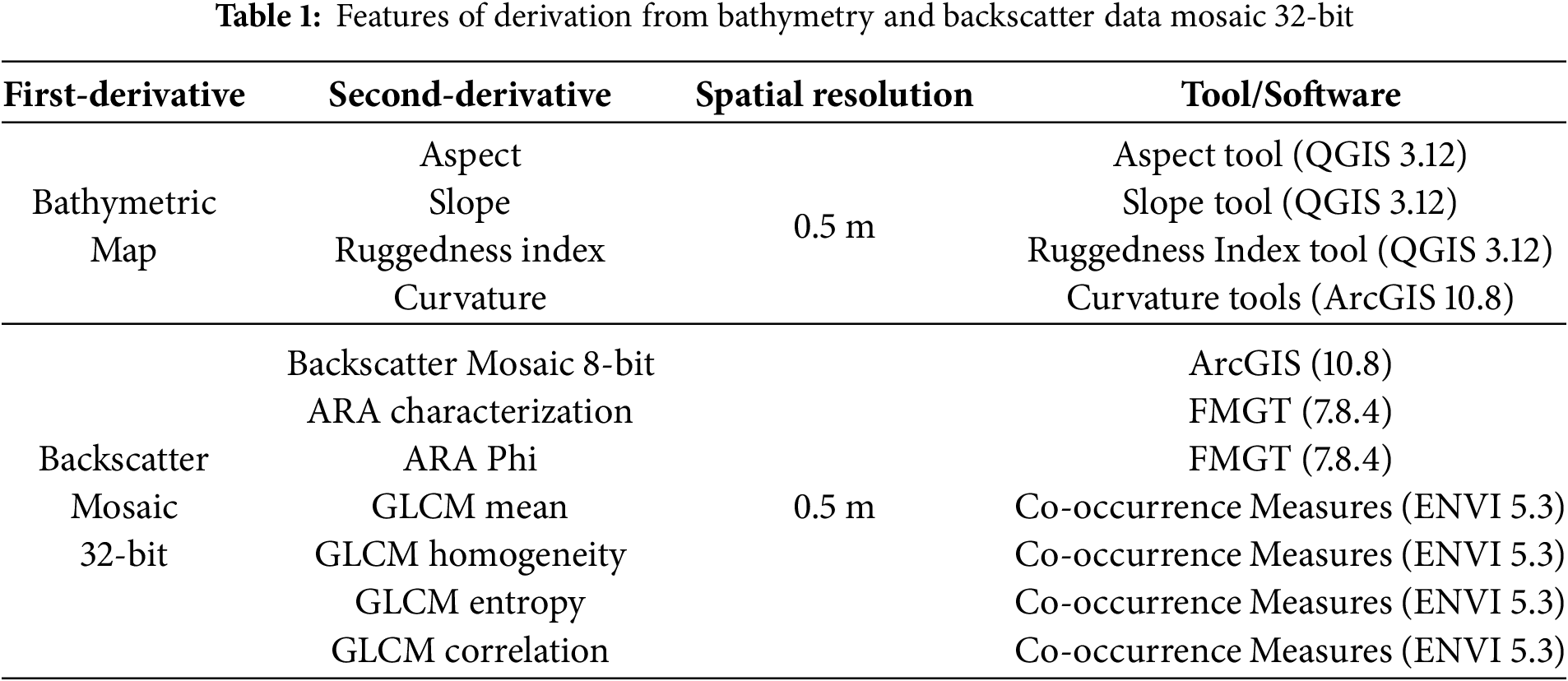
A thorough examination of the bathymetry and backscatter mosaic data is conducted in the next processing step. To identify subtle correlations and patterns, the second derivative of these datasets is computed. Aspect, slope, roughness index, and curvature are the four informative elements that are extracted from the bathymetry data through a series of changes. It is anticipated that these characteristics will offer insightful information on the shape and underlying structure of the seabed. In the meantime, several significant features are extracted from the 32-bit backscatter mosaic by processing, such as an 8-bit representation, ARA characterization, ARA phi, and a set of GLCM (Grey-Level Co-Occurrence Matrix) metrics, which encompass mean, homogeneity, entropy, and correlation. It is anticipated that the combined use of these derived features is anticipated to yield a more sophisticated understanding of the complex properties of the seabed environment.

Pearson’s correlation analysis is conducted to reveal the complex relationships between the backscatter attributes, such as mean, homogeneity, entropy, and correlation, and the various features that are extracted from the bathymetry and backscatter mosaic data, such as aspect, slope, ruggedness index, and curvature. By looking at correlations between these traits, patterns and interactions are found that may indicate underlying mechanisms or processes that form the seabed ecosystem. Certain characteristics, such as the roughness index and slope, are found to be significantly associated with one another, suggesting the presence of diverse seabed environments or habitats.

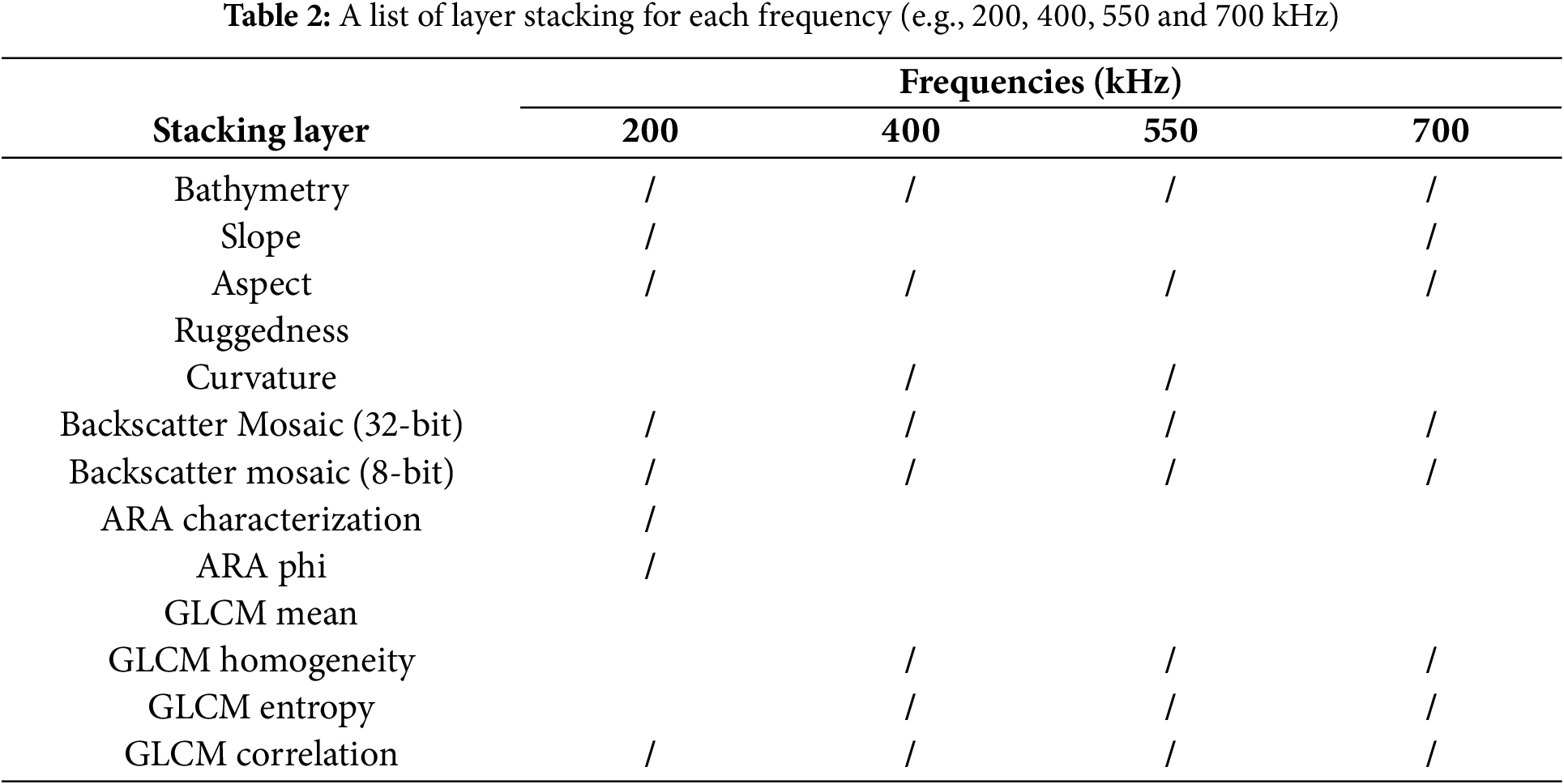
The method of determining the weak correlations between layers is carried out once all 13 layers from the first and second derivatives have been correlated. Once it is established that some layers have weak relationships with one another, these layers are chosen to be merged or stacked. The QGIS software is then utilized to stack or merge these weak layers, combining the selected layers into a single layer. The objective of this stacking or merging operation is to make the resulting classification model more predictive by reducing the dimensionality of the data. The stacked layers serve as input data for the supervised classification once they have all been constructed. Subsequently, the supervised classification is then conducted using a machine learning algorithm, which is trained on the stacked layers to identify patterns and relationships within the data.

2.7 Post-Processing

Through a complex fusion of data from various frequencies and a range of methodologies, the post-processing phase aimed to reveal specific sediment properties across the areas that have been surveyed by using the ML method. Two primary categorization models were specifically taken into consideration which is RF and SVM.

RF is a machine learning algorithm used for both regression and classification tasks. It utilizes ensemble learning, a technique that combines multiple classifiers to solve intricate problems [12]. This algorithm’s idea is derived from the structure of a collection of decision trees that are generated using a random dataset. Classification in this algorithm is carried out using the same methodology as the bagging algorithm, which is based on the classifier voting concept [13]. The RF regression involves increasing the number of trees for a given vector while treating the tree predictor, input parameters, and output parameters as numerical values. The training dataset is independently utilized for the random vector distribution. Hence, the computation of the mean-squared generalization error for the tree predictor is performed [14].

SVM learning is one of several approaches used in ML. SVM is highly proficient at identifying intricate patterns in complex datasets, often surpassing other ML algorithms in this regard [15]. They are extensively employed for classifying and estimating nonlinear functions. The SVM is a classification algorithm that is based on the idea of structural risk minimization. SVMs are systems that utilize a hypothesis space consisting of linear functions in a feature space with a high number of dimensions. These systems are trained using a learning algorithm derived from optimization theory, which incorporates a learning bias based on statistical learning theory. It takes into account both comprehensive risk and confidence risk, resulting in a high level of generalization ability [16].

3  Results and Analysis

3.1 First-Derivatives: Bathymetry Map and Backscatter Mosaic Map

Bathymetric data is collected using the Norbit iWBMS MBES with a multi-frequency ping base. A bathymetric map and backscatter mosaic map with multi-frequency results were generated. Different frequencies influence the resolution and coverage of the data. Figs. 4 and 5 illustrate the bathymetric and backscatter mosaic result with multi-frequency data generated to see the difference in the color of depth and decibels (dB) value for each frequency. There are four types of frequencies used in this study, e.g., 200, 400, 550, and 700 kHz. At 200 kHz for the bathymetry, the coverage area is the largest, making it ideal for extensive regions but with lower resolution, and missing finer details. The 400 kHz frequency offers improved resolution for capturing smaller features, though it covers a smaller area, increasing mapping time. At 550 kHz, there is a balance, providing intermediate resolution and coverage. The highest resolution is achieved at 700 kHz, capturing the smallest features but with the smallest coverage area, thus requiring the most time for data collection. This frequency has the highest resolution among the given frequencies, allowing it to capture even smaller features.

Figure 4: Bathymetry maps derived from multi-frequency MBES data

Figure 5: Backscatter mosaics derived from multi-frequency MBES data

Fig. 5 shows the result of the multi-frequency backscatter mosaic with the different scattering results captured at 200, 400, 550, and 700 kHz. Each frequency provides a different level of resolution and penetration depth, which affects the detection of seabed features and sediment types. The 400 kHz frequency offers higher resolution and scattering intensity than the 200 kHz, allowing it to capture smaller features and surface textures. The 550 kHz provides a balance between resolution and coverage, while the 700 kHz frequency delivers the highest resolution, enabling the detection of very fine textures.

Importantly, different sediment types respond uniquely to various acoustic frequencies. Coarser sediments such as sand and gravel typically generate stronger backscatter signals at lower frequencies (e.g., 200 kHz) due to their higher surface roughness and greater acoustic reflectivity. In contrast, finer sediments such as silt and mud tend to produce higher backscatter intensity at higher frequencies (e.g., 550–700 kHz) because of their smaller grain size and compact nature, which enhances sound wave scattering at short wavelengths [17]. Therefore, the variation in scattering intensity across frequencies in this mosaic also indicates the presence of different sediment types in the study area, supporting more detailed seabed classification.

3.2 Second-Derivative

The MBES dataset offers a comprehensive understanding of the underwater environment surrounding Waduk Selorejo. Through the analysis of this dataset, various derivatives are generated, including aspect, curvature, ruggedness index, curvature, 32-bit backscatter mosaic, 8-bit backscatter mosaic, ARA parameters, and GLCM texture features [18] (Table 1). These derivatives offer valuable insights into the study area, enabling the creation of a detailed bathymetric map that accurately represents the underwater topography. The backscatter mosaic, which represents the intensity of the returned acoustic signals, provides information on the seabed substrate and texture, with the 32-bit backscatter mosaic offering a more detailed representation of the acoustic signal intensity and the 8-bit backscatter mosaic providing a more visually appealing representation. Furthermore, the analysis of aspect, curvature, and ruggedness index, and curvature derivatives provides a deeper understanding of the seabed morphology and geological structures. Additionally, the application of texture-based analyses, including phi and characterization, correlation, entropy, homogeneity, and mean, enables the identification and classification of different seabed substrates based on their acoustic signatures. These findings are crucial in understanding the ecology and geology of the study area, as they provide valuable information on the seabed and the sediment that it supports, ultimately contributing to a more comprehensive understanding of the underwater environment and its ecosystems.

3.3 Correlation between Derivative

Pearson’s correlation analysis was conducted to uncover the complex relationships between the backscatter attributes, such as mean, homogeneity, entropy, and correlation, and the various features that are extracted from the bathymetry and backscatter mosaic data, such as aspect, slope, ruggedness index, and curvature. By looking at correlations among these traits, patterns, and interactions are found that may indicate the underlying mechanisms or processes shaping the seabed ecosystem. Notably, certain characteristics, such as the roughness index and slope, were found to be significantly associated with one another, suggesting the presence of diverse seabed environments or habitats. The analysis was performed in RStudio using the corrplot and RColorBrewer libraries in the R programming environment. The corrplot package was used to compute and visualize the correlation matrix, while RColorBrewer provided customized color palettes for better interpretability. The correlation analysis was performed using the cor function, and results were visualized as correlograms using the corrplot() function. This procedure was repeated separately for each of the four frequencies used in this study (e.g., 200, 400, 550, and 700 kHz) allowing an in depth assessment of frequency specific relationships between the extracted features (Fig. 6).

Figure 6: A correlogram was produced for each frequency (e.g., 200, 400, 550, and 700 kHz) in RStudio to display the correlation matrix and highlight the correlations between derivatives

The correlation coefficient, which measures the relationship between variables, determines the strength of the association. It is generally agreed upon that a correlation coefficient that is larger than or equal to 0.7, or less than or equal to −0.7, indicates a strong correlation, the correlation increases in strength as the coefficient approaches 1 or −1. When the coefficient lies in the range of 0.5 to 0.7, or between −0.5 and −0.7, it is said to have a moderate correlation. Conversely, a value between 0.3 and 0.5, or between −0.3 and −0.5, indicates a weak association. It is often considered that there is no significant link when the coefficient is less than 0.3 or more than −0.3. The method of determining the weak correlations between layers is carried out once all 13 layers from the first and second derivatives have been correlated. After it is established that some layers have weak relationships with one another, these layers are chosen to be merged or stacked. The goal of this stacking or merging operation is to make the resulting classification model more predictive by reducing the dimensionality of the data. The stacking layers (Table 2) are used as input data for the supervised classification once they have all been constructed.

3.4 Sediment Classification Map with Multi-Frequency

The sediment classification results obtained using a Random Forest machine learning method at four different frequencies, 200, 400, 550, and 700 kHz, exhibit a distinct pattern. As the frequency increases, the classification tends to identify finer sediment types. This trend is expected, as higher frequencies are more sensitive to smaller particles. At the lowest frequency of 200 kHz, the classification is dominated by coarser sediments such as gravel, coarse sand, and gravelly coarse sand, suggesting that the signal is primarily influenced by these larger particles. In contrast, the 400 kHz frequency reveals a broader range of sediments, including finer sands, silts, and even clay, indicating that the signal is beginning to capture the presence of smaller particles. As the frequency increases further to 550 and 700 kHz, the classification is predominantly composed of very fine silts, clays, and even sandy mud. This confirms that higher frequencies are highly sensitive to finer sediments, providing more detailed information about sediment composition. Notably, there is significant spatial variability in sediment classification at all frequencies, highlighting the heterogeneity of the sediment distribution and indicating that sediment type varies across the area being studied (Fig. 7).

Figure 7: Sediment map classified by using Random Forest

The sediment classification results obtained using the Support Vector Machine (SVM) method at four different frequencies, 200, 400, 550, and 700 kHz exhibit a distinct pattern. As the frequency increases, the classification becomes more detailed, transitioning from coarser to finer sediment types. At the lowest frequency of 200 kHz, the classification is dominated by coarse-grained sediments like “Gravel” and “Coarse Sand”, suggesting that the signal is primarily influenced by larger particles. In contrast, at higher frequencies, finer-grained sediments like “Fine Silt”, “Clay”, and “Sandy Clay” become more prevalent, indicating that the signal is capturing the presence of smaller particles.

The 400 kHz frequency adds more detail to the classification, with the appearance of “Fine Silt” and “Very Fine Sand” classes, while still detecting some larger materials. The 550 kHz frequency offers an even finer distinction, with the emergence of “Sandy Mud” and “Medium Sand-Gravelly Muddy Sand” classes, suggesting the presence of muddy sediments mixed with sand and gravel. Finally, the highest frequency of 700 kHz uncovers the most intricate details, with the presence of “Silty Clay” and “Sandy Clay” classes, indicating a significant presence of fine-grained, clay-rich sediments. The results can be attributed to the differences in penetration depth and wave interactions among the frequencies. Higher frequencies have a shallower penetration depth, making them more sensitive to subtle variations in texture and composition within fine-grained sediments. The SVM method has effectively captured these differences, providing a more comprehensive understanding of the sediment composition and structure (Fig. 8).

Figure 8: Sediment map classified by using Support Vector Machine

3.5 Accuracy Assessment

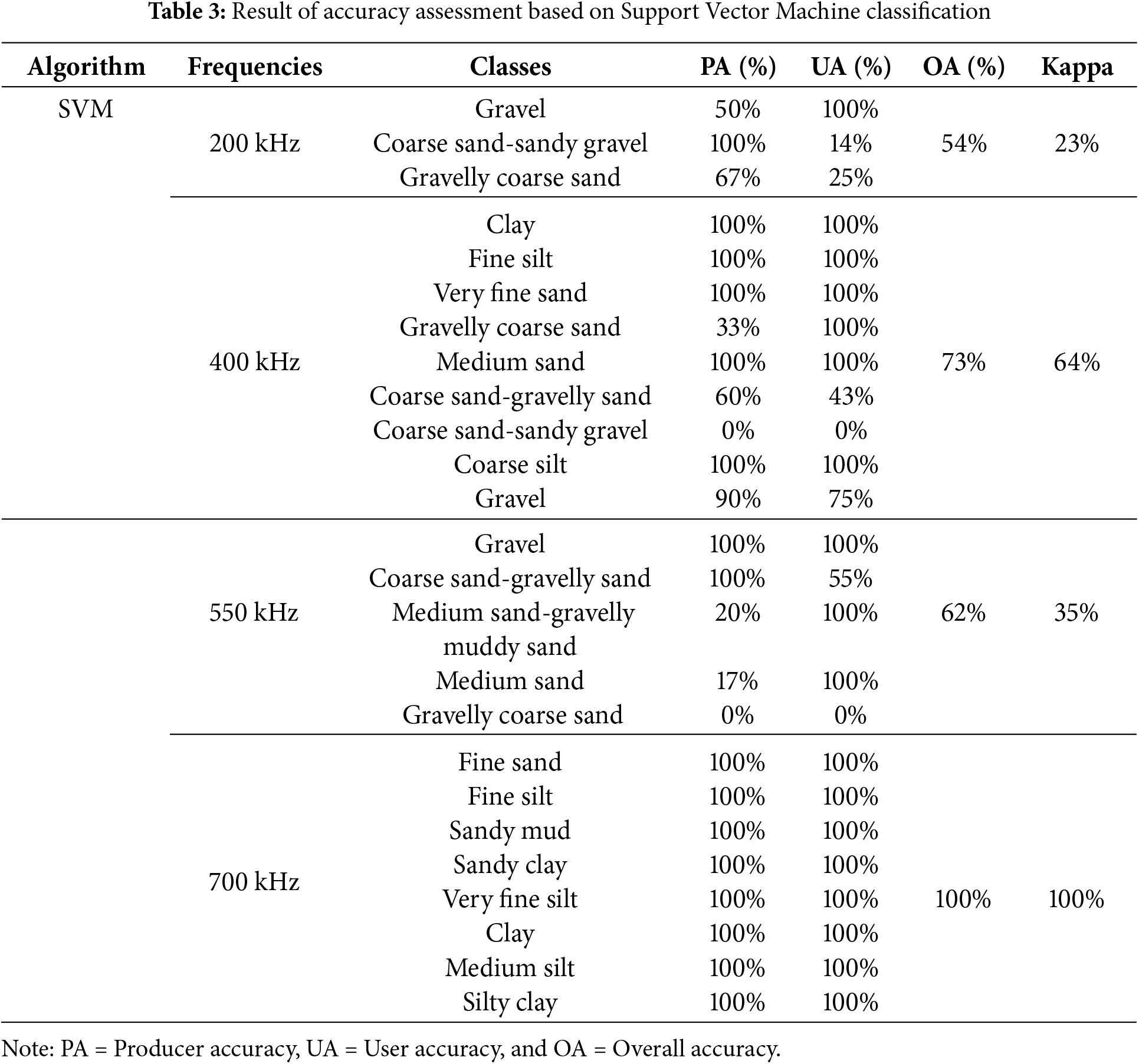
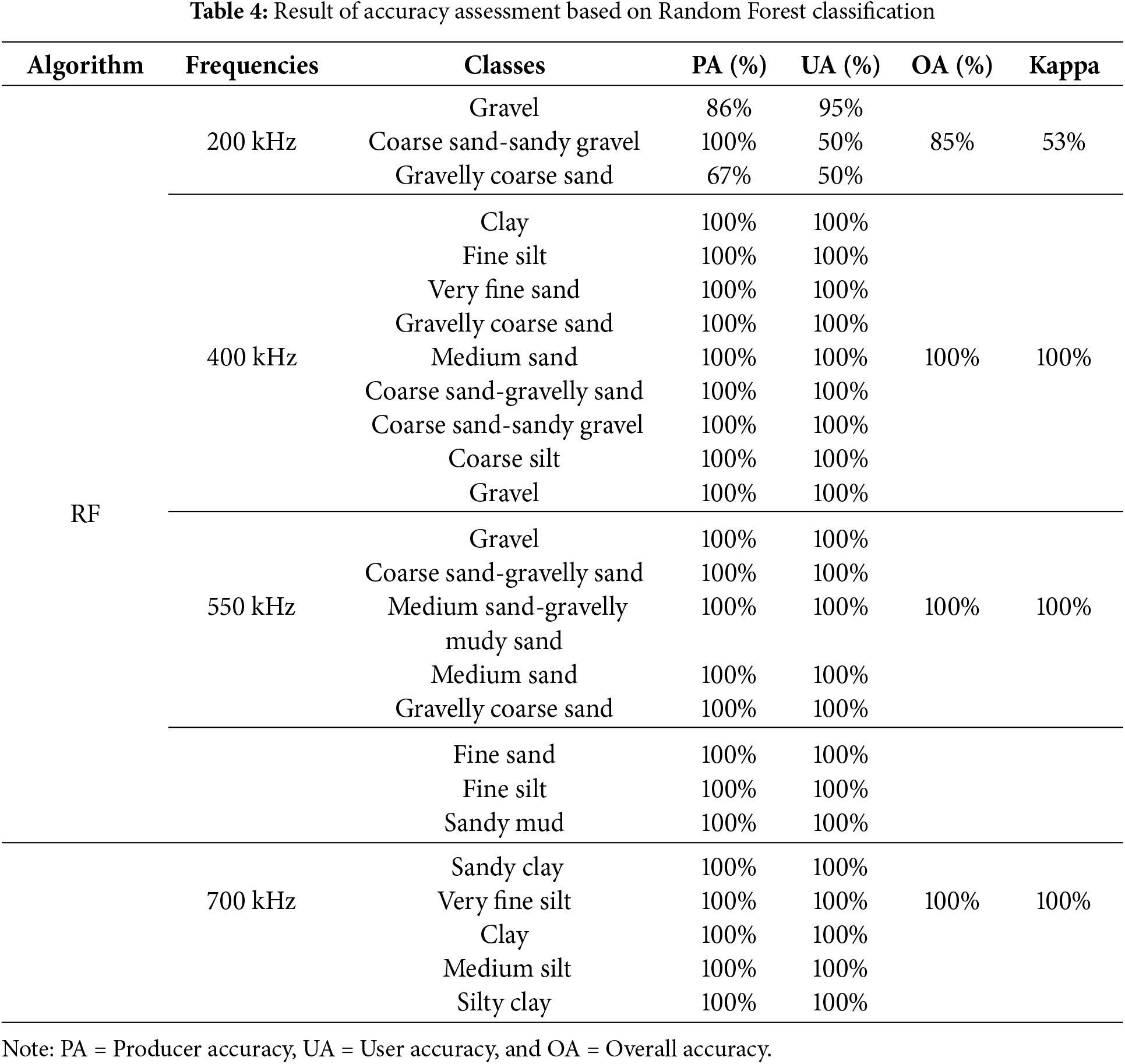
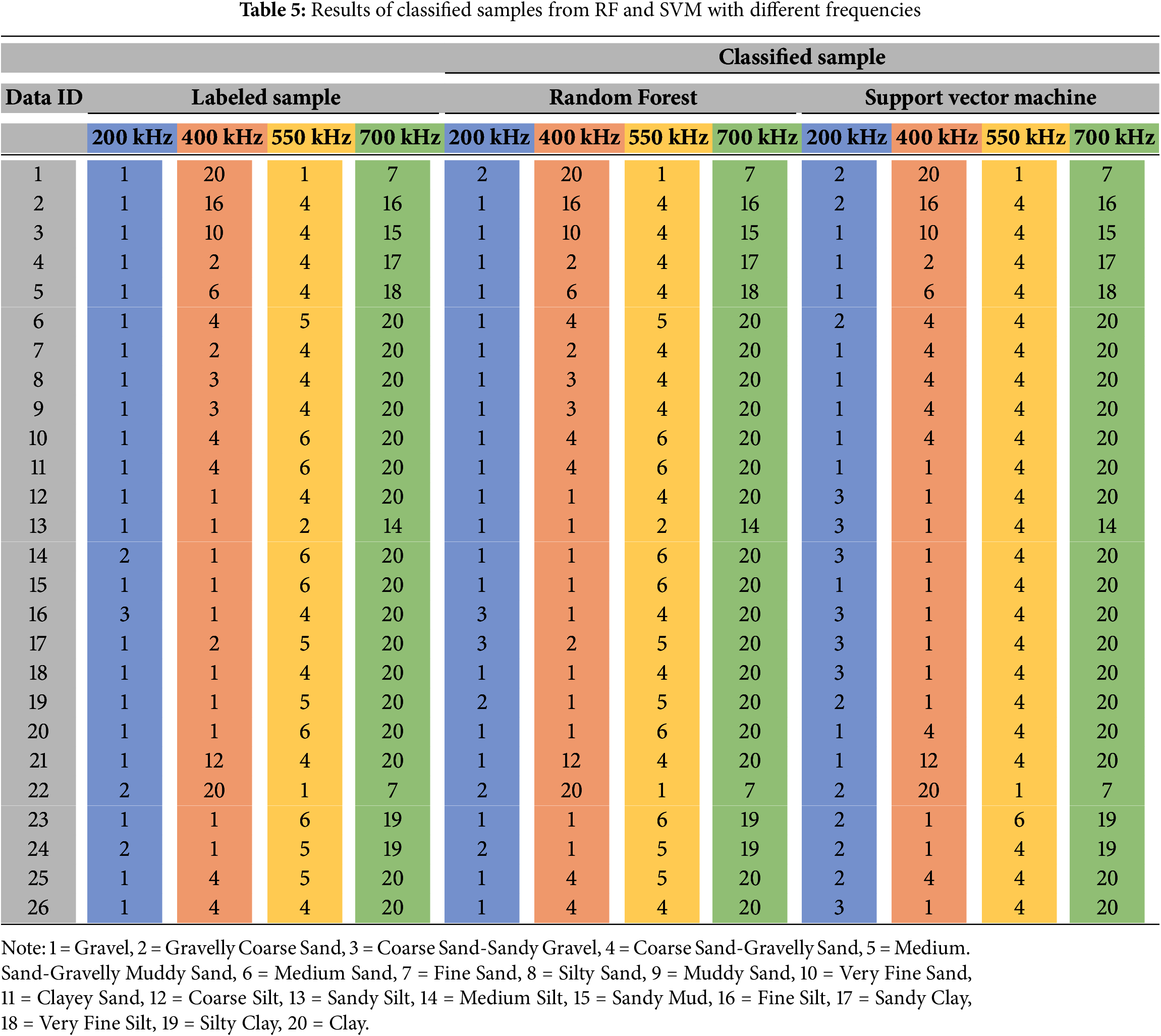
According to the results of the accuracy assessment (Tables 3 and 4), the Support Vector Machine (SVM) classification performs better overall than the Random Forest classification for most frequency types. SVM performs incredibly well at 400 kHz with an accuracy of 90%, but struggles at 550 kHz with an accuracy of 73%. The accuracy varies depending on the type of frequency. This frequency dependence implies that each frequency type’s unique properties have an impact on the categorization methods. A closer look reveals that there are notable differences in accuracy amongst the classes. The algorithms can discriminate between the “Gravel” and “Coarse Sand-Sandy Gravel” classifications, since they are consistently identified with high accuracy across all frequency types. On the other hand, the “Clay” and “Silty Clay” groups have lower accuracy rates and are more difficult to classify. The differences in accuracy between classes could be explained by the intrinsic qualities of each class, with some being easier to distinguish from others. Table 5 shows the result of classified samples from different frequencies (e.g., 200, 400, 550 and 700 kHz). The numbers from the table are representative of each sediments class from FMGT ARA characterization library.

4  Discussions

The incorporation of multi-frequency MBES technology, ground-truth data, and machine learning algorithms to create a sediment map for Waduk Selorejo, Indonesia, was explored in this study. This research represents one of the first attempts to employ these techniques for sediment classification in a freshwater reservoir. The results of the study demonstrate the effectiveness of using multi-frequency MBES data and machine learning algorithms to identify and classify different sediment types.

The sediment classification results obtained using the RF and SVM methods at four different frequencies (200, 400, 550, and 700 kHz) exhibit a distinct pattern. As the frequency increases, the classification tends to identify finer sediment types, which is expected since higher frequencies are more sensitive to smaller particles. Furthermore, the outputs demonstrated significant spatial variability in sediment distribution across all frequencies, highlighting the heterogeneous nature of the reservoir floor and suggesting that sediment deposition in freshwater reservoirs is influenced by a combination of hydrodynamic, geomorphological, and anthropogenic factors [19–21].

The use of multi-frequency MBES data and machine learning algorithms offers several advantages over traditional sediment classification methods. Firstly, the high-resolution bathymetric and backscatter data provided by the MBES system allow for a more detailed understanding of the underwater environment. Secondly, the machine learning algorithms can handle large datasets with multiple variables, making them ideal for analyzing the complex relationships between the MBES data and sediment characteristics. To ensure statistical robustness in variable selection, a Pearson correlation coefficient analysis was conducted to identify and retain only the most relevant and non-redundant input features. This step minimized multicollinearity and ensured that the selected variables contributed meaningfully to the classification models. Finally, the use of multi-frequency data enables the identification of finer sediment types, which is essential for understanding the ecological and geological processes in freshwater reservoirs.

The findings of this study have several implications for sediment management and conservation in freshwater reservoirs. The sediment map generated from this research can be utilized to identify areas with high sedimentation rates based on the geographical distribution of fine-grained sediments such as silt and mud, categorised using multifrequency MBES data. These areas are often associated with low hydrodynamic energy zones, such as those near river inlets, deeper basin regions, and areas with minimal water flow. The view is further reinforced by analyzing reservoir-specific features such as input direction, water circulation patterns, and bathymetric depressions, all of which affect sediment transport and deposition [22,23]. This can guide management decisions regarding sediment removal and habitat restoration. Additionally, the study’s results can be employed to develop more effective conservation strategies for freshwater reservoirs, such as identifying regions with high biodiversity and ensuring their protection from excessive sedimentation that may degrade habitat quality and ecological function.

Although this study primarily focuses on sediment mapping for reservoir management, the integration of multi-frequency MBES data and detailed backscatter analysis may also have potential applications in hydrographic chart production. The spatial distribution of sediment types, particularly when classified using robust machine learning algorithms, provides supplementary information that can enhance environmental layers in hydrographic products. For instance, seabed type and roughness can inform decisions related to anchorage, underwater construction, or ecological zoning. While this study does not directly aim to produce hydrographic charts, the methodology and findings presented may support future efforts to enrich hydrographic surveys with sedimentological insights, particularly in freshwater or inland navigation contexts.

5  Conclusions

This study utilized multi-frequency multibeam echosounder (MBES) technology, ground-truth data, and machine learning algorithms to create a sediment map for Waduk Selorejo, Indonesia. The results demonstrate the effectiveness of using multi-frequency MBES data and machine learning algorithms to identify and classify different sediment types, including gravel, coarse sand, fine sand, silt, and clay. The study’s findings highlight the importance of considering the frequency-dependent characteristics of MBES data and the advantages of using machine learning algorithms for analyzing complex datasets.

Consequently, this study concludes that the Random Forest and Support Vector Machine algorithms are useful in categorizing the distribution of sediment types in freshwater reservoirs. As this is an initial study conducted to develop sediment maps in the study area, further research is required in the future, which should incorporate various machine learning algorithms and explore the application of sediment maps in freshwater reservoir management and conservation. Creating an accurate map of sediment distribution is crucial for understanding the ecological and geological processes in freshwater reservoirs, particularly in the face of human activities and environmental changes.

It is important to note that the ground truth data used in this study was limited, as direct sediment sampling from the field was not available. Instead, sediment classification relied on representative samples derived from Angular Range Analysis (ARA), which served as pseudo ground truth data for model training and validation. While this approach provided valuable insight, the absence of field-verified sediment samples may affect the accuracy and reliability of the classification results. Future work should incorporate field-verified sediment samples to enhance classification accuracy and improve the reliability of sediment maps for practical decision making.

Acknowledgement: The authors would like to thank the Sepuluh Nopember Institute of Technology, for the acoustic data collection. Special thanks to the team partners from PT. Sonar Nusantara Utama. We are also grateful for the reviews, comments, and suggestions from three reviewers for improving our manuscript.

Funding Statement: The authors received no specific funding for this study.

Author Contributions: The authors confirm contribution to the paper as follows: Conceptualization, Qaisara Yusriena Yusaini, Muhammad Abdul Hakim Muhamad, Raiz Razali, Rozaimi Che Hasan, Mohd Zainee Mohd Zainal; methodology, Qaisara Yusriena Yusaini, Muhammad Abdul Hakim Muhamad, Ikhsan Nuradi; software, Qaisara Yusriena Yusaini, Muhammad Abdul Hakim Muhamad, Ikhsan Nuradi; validation, Raiz Razali, Mohd Shahmy Mohd Said; writing—original draft preparation, Qaisara Yusriena Yusaini, Muhammad Abdul Hakim Muhamad; writing—review and editing, Qaisara Yusriena Yusaini, Muhammad Abdul Hakim Muhamad, Raiz Razali; visualization, Mohd Shahmy Mohd Said; project administration, Ikhsan Nuradi. All authors reviewed the results and approved the final version of the manuscript.

Availability of Data and Materials: Data available within the article. The authors confirm that the data supporting the findings of this study are available within the article.

Ethics Approval: Not applicable.

Conflicts of Interest: The authors declare no conflicts of interest to report regarding the present study.

References

1. Brown CJ, Beaudoin J, Brissette M, Gazzola V. Multispectral multibeam echo sounder backscatter as a tool for improved seafloor characterization. Geosciences. 2019;9(3):126. doi:10.3390/geosciences9030126. [Google Scholar] [CrossRef]

2. Wan J, Qin Z, Cui X, Yang F, Yasir M, Ma B, et al. MBES seabed sediment classification based on a decision fusion method using deep learning model. Remote Sens. 2022;14(15):3708. doi:10.3390/rs14153708. [Google Scholar] [CrossRef]

3. Misiuk B, Brown CJ. Benthic habitat mapping: a review of three decades of mapping biological patterns on the seafloor. Estuar Coast Shelf Sci. 2024;296(1983):108599. doi:10.1016/j.ecss.2023.108599. [Google Scholar] [CrossRef]

4. Ji X, Yang B, Tang Q. Seabed sediment classification using multibeam backscatter data based on the selecting optimal random forest model. Appl Acoust. 2020;167(2):107387. doi:10.1016/j.apacoust.2020.107387. [Google Scholar] [CrossRef]

5. Wang H, Zhou Q, Wei S, Xue X, Zhou X, Zhang X. Research on seabed sediment classification based on the MSC-transformer and sub-bottom profiler. J Mar Sci Eng. 2023;11(5):1074. doi:10.3390/jmse11051074. [Google Scholar] [CrossRef]

6. Linklater M, Ingleton T, Kinsela M, Morris B, Allen K, Sutherland M, et al. Seabed classification approach for SeaBed NSW coastal seafloor mapping program. In: Proceedings of the HYDRO18 Conference; 2018 Oct 30–Nov 1; Sydney, Australia. [Google Scholar]

7. Runya RM, McGonigle C, Quinn R, Howe J, Collier J, Fox C, et al. Examining the links between multi-frequency multibeam backscatter data and sediment grain size. Remote Sens. 2021;13(8):1539. doi:10.3390/rs13081539. [Google Scholar] [CrossRef]

8. Nitriansyah R, Cahyono BK. Seabed classification using multibeam echosounder measurement data. IOP Conf Ser Earth Environ Sci. 2022;1039(1):012045. doi:10.1088/1755-1315/1039/1/012045. [Google Scholar] [CrossRef]

9. Hewitt AT, Salisbury R, Wilson J. Applications of multibeam backscatter: using multibeam echosounder backscatter to characterize and map seafloor features in shallow and deep water. In: Proceedings of the Offshore Technology Conference; 2010 May 3–6; Houston, TX, USA. doi:10.4043/20672-ms. [Google Scholar] [CrossRef]

10. Gaida TC, Tengku Ali TA, Snellen M, Amiri-Simkooei A, Van Dijk TAGP, Simons DG. A multispectral Bayesian classification method for increased acoustic discrimination of seabed sediments using multi-frequency multibeam backscatter data. Geosciences. 2018;8(12):455. doi:10.3390/geosciences8120455. [Google Scholar] [CrossRef]

11. Samsudin SA, Hasan RC. Assessment of multibeam backscatter texture analysis for seafloor sediment classification. Int Arch Photogramm Remote Sens Spatial Inf Sci. 2017;42:177–83. doi:10.5194/isprs-archives-xlii-4-w5-177-2017. [Google Scholar] [CrossRef]

12. Mbaabu. Introduction to Random Forest in Machine Learning: section; 2020. [Internet]. [cited 2023 Nov 3]. Available from: https://www.section.io/engineering-education/introduction-to-random-forest-in-machine-learning/#:~:text=The%20rain%20forest%20algorithm%20is,problem%20of%20overfitting%20of%20datasets. [Google Scholar]

13. Kogut T, Weistock M. Classifying airborne bathymetry data using the Random Forest algorithm. Remote Sens Lett. 2019;10(9):874–82. doi:10.1080/2150704X.2019.1629710. [Google Scholar] [CrossRef]

14. Azimi H, Shiri H, Mahdianpari M. Iceberg-seabed interaction analysis in sand by a random forest algorithm. Polar Sci. 2022;34(5):100902. doi:10.1016/j.polar.2022.100902. [Google Scholar] [CrossRef]

15. Huang S, Cai N, Pacheco PP, Narrandes S, Wang Y, Xu W. Applications of support vector machine (SVM) learning in cancer genomics. Cancer Genom Proteom. 2018;15(1):41–51. doi:10.21873/cgp.20063. [Google Scholar] [PubMed] [CrossRef]

16. Cui X, Liu H, Fan M, Ai B, Ma D, Yang F. Seafloor habitat mapping using multibeam bathymetric and backscatter intensity multi-features SVM classification framework. Appl Acoust. 2021;174(10):107728. doi:10.1016/j.apacoust.2020.107728. [Google Scholar] [CrossRef]

17. Brown CJ, Cooper KM, Meadows WJ, Limpenny DS, Rees HL. Small-scale mapping of sea-bed assemblages in the eastern English channel using sidescan sonar and remote sampling techniques. Estuar Coast Shelf Sci. 2002;54(2):263–78. doi:10.1006/ecss.2001.0841. [Google Scholar] [CrossRef]

18. Muhamad MH, Che Hasan R. Seagrass habitat suitability models using multibeam echosounder data and multiple machine learning techniques. IOP Conf Ser Earth Environ Sci. 2022;1064(1):012049. doi:10.1088/1755-1315/1064/1/012049. [Google Scholar] [CrossRef]

19. Gonzalez Rodriguez L, McCallum A, Kent D, Rathnayaka C, Fairweather H. A review of sedimentation rates in freshwater reservoirs: recent changes and causative factors. Aquat Sci. 2023;85(2):60. doi:10.1007/s00027-023-00960-0. [Google Scholar] [CrossRef]

20. Li Y, Gao B, Xu D, Peng W, Liu X, Qu X, et al. Hydrodynamic impact on trace metals in sediments in the cascade reservoirs, North China. Sci Total Environ. 2020;716(22):136914. doi:10.1016/j.scitotenv.2020.136914. [Google Scholar] [PubMed] [CrossRef]

21. Liu D, Lin Y, Zhang T, Huang E, Zhu Z, Jia L. Impact of anthropogenic activities on sedimentary records in the Lingdingyang Estuary of the Pearl River Delta. China J Mar Sci Eng. 2024;12(7):1139. doi:10.3390/jmse12071139. [Google Scholar] [CrossRef]

22. Shaw JB, Mohrig D, Wagner RW. Flow patterns and morphology of a prograding river delta. J Geophys Res Earth Surf. 2016;121(2):372–91. doi:10.1002/2015JF003570. [Google Scholar] [CrossRef]

23. Herrero A, Bateman A, Medina V. Water flow and sediment transport in a 90° channel diversion: an experimental study. J Hydraul Res. 2015;53(2):253–63. doi:10.1080/00221686.2014.989457. [Google Scholar] [CrossRef]