Dynamic Coefficient Triangular Greenness Index for Aerial Phenotyping in a Liberica Coffee Farm

1  Introduction

Unmanned Aerial Systems (UAS) have attracted significant attention in applications related to smart farming [1,2]. More and more sophisticated instruments are now being incorporated as payloads to monitor crop conditions and growth [3]. Among the techniques used to gauge the status of crops from an airborne surveillance system is phenotyping. It is the process of extracting the physiological traits of crops, including shape, color, and canopy size [4]. One parameter in phenotyping that significantly provides insight into the status of crop health is the chlorophyll estimates [5,6]. Greenness serves as an indirect indicator of chlorophyll content in leaves, as it results from light reflectance that correlates with chlorophyll levels.

Researchers can estimate chlorophyll content using several vegetation indices derived from leaf spectral reflectance, such as the Normalized Difference Vegetation Index (NDVI), the Modified Chlorophyll Absorption Ratio Index (MCARI), the Chlorophyll Index–Red Edge (CIred-edge), among others [7]. However, most vegetation indices require sensors capable of detecting spectral reflectance beyond the visible range—such as in the near-infrared—which cannot be captured by standard RGB cameras. Multispectral and hyperspectral cameras are commonly employed in remote sensing and precision agriculture for this purpose [8]. These cameras capture reflectance data in multiple narrow spectral bands to analyze vegetation health, water stress, and other surface characteristics [9]. The well-characterized spectral sensitivity of each band allows for accurate interpretation and calibration of the sensor’s spectral response. Although multispectral and hyperspectral cameras are available, RGB imaging devices offer a more accessible alternative for estimating chlorophyll concentrations in plants. Most UAS platforms are already equipped with such imaging devices and require no additional alteration to the payload for crop monitoring. However, the direct use of RGB images to represent chlorophyll estimates is greatly affected by the natural lighting conditions, which are significantly dynamic. Researchers have proposed manipulation of the RGB channels or transformations into different color spaces to derive alternative vegetation indices correlated to chlorophyll content. One widely considered index used to estimate chlorophyll content is the Triangular Greenness Index (TGI) [10], which uses the triangle formed by the reflectance response curve. Mathematically, Eq. (1) defines TGI:

TGI=−0.5[(λRed−λBlue)(RRed−RGreen)−(λRed−λGreen)(RRed−RBlue)](1)

where R denotes the reflectance at the specified wavelength λ.

However, the image sensor to be used must have a known spectral response to compute the TGI value accurately. The lack of knowledge on the spectral response of the RGB imaging devices installed in unmanned aerial vehicles (UAVs) poses a problem since they vary across different manufacturers. Most of the time, the spectral response of these cameras is not included in the specification of the drone itself. De Ocampo et al. [11] proposed a method to simplify TGI derivation by combining the spectral response variables from the original equation into two coefficients defined through a parametric sweep from 400 to 700 nm. However, once the TGI is calibrated based on the spectral characteristics of the sensor, the resulting equation becomes fixed and cannot be adjusted during subsequent analyses. In addition, the previous study didn’t include validation on chlorophyll estimates. Table 1 provides the pragmatic benefits of RGB-based chlorophyll estimation over SPAD measurements.

This study proposes a framework for aerial phenotyping that uses a modified version of the TGI equation with adjusted coefficients. Accurate chlorophyll estimation provides essential insights into plant health and nutrient status, which is the main objective of phenotyping. However, this study focuses on post-processing of the aerial images rather than real-time assessment using UAVs, as implemented in the work of Bakirci [12].

2  Literature Review

Phenotyping can improve crop management by allowing farmers to assess plant traits related to growth, stress tolerance, and yield potential [13]. Phenotyping offers a non-destructive approach to determine a plant’s response to environmental stresses. There is a plethora of trait measures in physiological phenotyping for plants, such as chlorophyll content, stomatal conductance, photosynthetic rate, leaf area index, water use efficiency, and biomass accumulation.

Among these physically measurable traits, chlorophyll estimation is particularly significant, as it serves as an indicator of plant health, nitrogen status, and photosynthetic efficiency [14]. Accurate chlorophyll measurement allows for better nutrient management and precision agriculture practices, which aim to improve crop productivity and sustainability. Although conventional phenotyping methods are well established and reliable, they heavily rely on labor-intensive and time-consuming manual measurements. Researchers have traditionally estimated chlorophyll using tools such as SPAD meters, spectrophotometers, and destructive sampling techniques [15]. These approaches, while accurate, require significant resources and may not be feasible for large-scale agricultural assessments. Similarly, leaf count and coverage have historically been measured through manual field surveys, limiting the efficiency and scalability of phenotypic evaluations [16]. Remote sensing technologies used in phenotyping have been around for the last two decades and are steadily gaining promising results toward more efficient phenotyping tasks. The use of UAS gained popularity in field studies due to their increasing efficiency, and this is also true in phenotyping. Aerial phenotyping using UAS enables larger coverage and rapid implementation.

UAS platforms include not only UAVs but also the ground station, payload, and necessary communication links. Specific to the payload, recent advancements in sensor technologies have allowed the implementation of multi-and hyperspectral imaging devices in a much smaller form factor, making the weight suitable for UAS. Satellites can also carry similar spectral sensor systems, but they drastically reduce spatial resolution and significantly increase equipment costs [17]. The bottleneck in cost and spatial resolution imposed by satellite implementations of these remote sensing systems makes UAS a more preferred solution for aerial phenotyping. UAS-based phenotyping enables rapid and cost-effective phenotyping and also provides high-resolution, large-scale data collection, while reducing the need for manual labor and improving measurement consistency. The high-throughput phenotyping using spectral sensors makes use of plants’ reflectance signatures that vary significantly due to biotic and abiotic stresses [18]. Manipulation of raw spectral measurements to derive another metric, commonly referred to as vegetation indices (VIs), enables researchers to squeeze more meaningful information. The transformed radiation values reflected from surfaces can enhance or highlight specific traits of the target plants, such as chlorophyll content, water stress, vegetation, and canopy covers. Each VI has its advantages and disadvantages. An example is NDVI, which is well known to distinguish vegetation (0.1 to +1.0) from water (−1.0 to −0.1) and soil (−0.1 to 0.1) [19]. However, NDVI is very sensitive to errors due to varying atmospheric conditions [20]. Soil reflectance or background can influence NDVI, but combining NDVI with other vegetation indices helps mitigate this effect [21]. The Green Normalized Difference Vegetation Index (GNDVI) is computed similarly to NDVI but uses the green channel instead of the red band to enhance sensitivity to chlorophyll contents [19]. Other vegetation indices were improvements of NDVI, such as Soil-Adjusted Vegetation Index (SAVI) and Transformed Chlorophyll Absorption in Reflectance Index (TCARI) [22]. Fortunately, the visible spectrum is among the wavelength ranges where plants exhibit high reflectance. A more interesting group of VIs is those derived from RGB channels or the visible spectrum. Among these VIs are Excess Green Index (ExG), Excess Red Index (ExR), Photochemical Reflectance Index (PRI), Modified Green Red Vegetation Index (MGRVI), TGI, and Visible Atmospherically Resistant Index (VARI), to name a few. ExG enhances vegetation contrast to soil [23] while MGRVI highlights green variation from red, which is robust against variation in soil background. ExR enhances red reflectance to detect stressed vegetation using RGB images [24], while the PRI utilizes narrow-band spectral data to assess photosynthetic efficiency for physiological stress monitoring [25]. For vegetation detection, TGI and VARI perform well, with the latter being more robust in atmospheric variations. However, TGI is more suitable for chlorophyll estimation using RGB reflectance.

Due to the accessibility of RGB imaging devices, most researchers recognize TGI as an alternative to VIs derived from multispectral sensors. The study of [26] investigates the application of the TGI as a spectral indicator to assess dicamba-induced phytotoxicity in soybean (Glycine max). The study concludes that TGI is a practical tool for the early detection of herbicide-induced stress in soybean cultivation without using multispectral imaging devices. Aside from plant stress, the use of TGI in the detection of fungal-related disease showed promise as demonstrated in [27]. The study used aerial images of pine trees and examined the variations in greenness in the tree foliage. Fungal infestation makes pine leaves dry, which is particularly evident in aerial images with the implementation of TGI. In another study [28], the TGI is used in canopy area estimation in hop gardens, which also validates the potential of using RGB-based vegetation indices, particularly TGI, in improved monitoring and management in precision agriculture.

3  Methods

3.1 Acquisition of Aerial Images of Liberica Coffee Seedling

The study took place on a 5000 square meter demonstration farm for Liberica coffee seedlings in Batangas, Philippines. The demonstration farm contains at least 500 coffee seedlings spaced at a 3-m separation, where 50 plants were sampled randomly for SPAD measurements. Tagged positions of the identified sample plants served as reference points during aerial image annotation. Each seedling measured yields three readings, taken from the bottom, middle, and top leaves. Aside from the SPAD measurements, the study collected digital aerial images of the sampled plants using the camera native to the UAV. Fig. 1 is a sample aerial image of Liberica coffee seedlings.

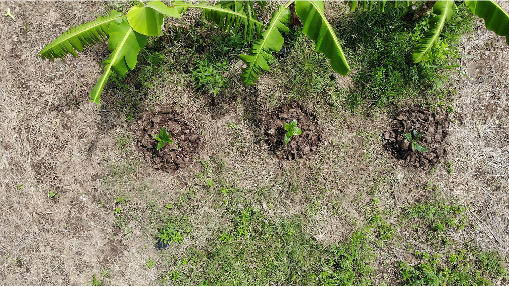
Figure 1: Sample aerial image of coffee seedlings

Frame extraction yielded 3420 raw images from 14 aerial videos recorded at a 30-m altitude, with durations ranging from 17 to 288 s. The training phase used 70% of the images collected, while validation and testing used the remaining 30%. The previously selected 50 seedlings were annotated from the collected images to match them to the manually acquired SPAD measurements. Additionally, the sampling rate for the raw videos is 23.98 frames/sec, with a frame size of 3840 × 2160 pixels at 96 dpi. The UAV used is DJI Mavic Air equipped with 2375 mAh battery and an RGB camera system consisting of a sensor (1/2.3″ CMOS), 3-axis image stabilizer, 4K Ultra HD (3840 × 2160 24/25/30p), with a lens of 85∘ field of view (FOV), 35 mm format equivalent to 24 mm, and an effective pixel of 12 MP. The mobile device control operates at a frequency of 2.400–2.4835 GHz.

3.2 Pre-Processing of Aerial Images

The collected frames from the aerial videos served two purposes: training the plant detection model (1) and testing the algorithm for aerial phenotyping using the proposed Dynamic Coefficient Triangular Greenness Index or DCTGI (2). The plant detection model, based on YOLO, trains on images annotated with two labels: ‘positive’ for regions containing coffee seedlings and ‘negative’ for all other areas (Fig. 2). The exact number of ‘negative’ and ‘positive’ regions was labeled in each image to make the dataset balanced. Suppose that the aerial image doesn’t contain any coffee seedlings, the dataset discards it. This study used a YOLO-based plant detection model based on the work of [29]. The YOLO-based model training used a lightweight configuration in MATLAB to automate the detection of all seedlings across multiple aerial images. The process resized input images to 227 × 227 × 3 and estimated six anchor boxes using k-means clustering on the ground truth data. These anchors were sorted by area and divided into two detection scales. SqueezeNet served as the base network, with feature maps from the ‘fire5-concat’ and ‘fire9-concat’ layers used for multi-scale detection. The training data underwent augmentation and preprocessing specific to the detector. The training ran for 80 epochs with a mini-batch size of 8, a learning rate of 0.001, and a warm-up period of 1000 iterations. L2 regularization (0.0005) and an IoU penalty threshold of 0.5 were applied to improve generalization and refine positive match criteria. The second purpose covers the calculation of the DCTGI from the cropped images of coffee seedlings. However, only the tagged seedlings were included in the DCTGI analysis, as these were the ones with corresponding SPAD measurements. The annotation also includes leaf count and coverage.

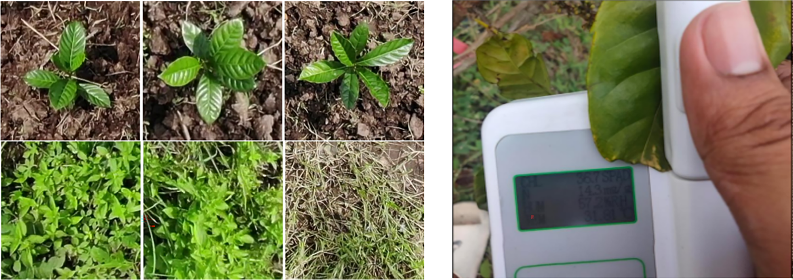
Figure 2: ‘Positive’ (top) and ‘Negative’ (bottom) samples from the training data (left). SPAD meter used for ground-truth (right)

3.3 Reconstruction of Dynamic Coefficient Triangular Greenness Index for Chlorophyll Estimation

The TGI, as defined in [10,30], is a geometric relationship between the reflectances of red (R), green (G), and blue (B) bands. It calculates the area of the triangle created by the three reflectances. However, the reflectance space used to calculate TGI is very sensitive to the spectral response of the sensors used. The challenge in the use of the original TGI is that the wavelength of the camera device must be known to calculate the TGI value. When implemented with a new camera, the TGI estimate cannot adapt to the new spectral response of the camera sensor. The point of improvement to the original TGI is the introduction of dynamic coefficients (α,β) for representing the spectral response of the sensor used. In this study, these coefficients vary depending on the calibration readings for the imaging devices used by the UAV.

Recalibration in the proposed DCTGI used a reference chart with a known TGI value equivalent, which reduces the need to know the spectral responses of the CMOS or CCD sensors used. A standard leaf color chart, as shown in Fig. 3, is used as a reference.

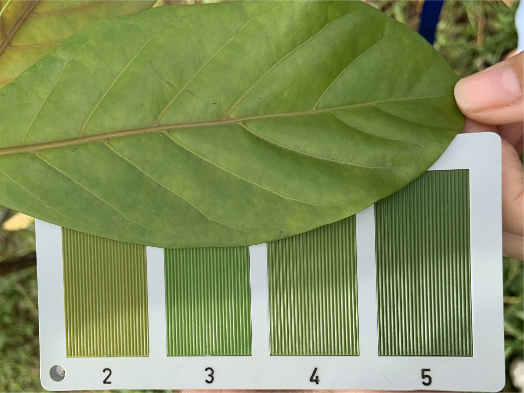
Figure 3: Standard leaf color chart used to calibrate DCTGI

The TGI value calculated on the image of the leaf color chart captured using a spectral camera (Micasense RedEdge MX) with known spectral responses is then compared to the calculated DCTGI value on the same leaf color chart image captured using another RGB camera (Samsung Galaxy Flip Z3 camera with unknown wavelengths). The coefficients of Eq. (2) can then be adjusted to arrive at the nearest value to the original TGI. Eqs. (3) and (4) show how the previously known reflectances are combined.

DCTGI=RGreen−αRRed−βRBlue(2)

α=2(λBlue−λGreen)(λBlue−λRed)(3)

β=2(λGreen−λRed)(λBlue−λRed)(4)

Bhattacharyya distance is calculated on the band images of the leaf color chart at different lighting conditions to validate that the reflectance distribution of the spectral camera employed is consistent under varying illumination or lighting conditions [31]. The pixel intensity distribution represents the reflectance of the sensors in the multispectral camera since the process didn’t include radiometric calibration. Fig. 4 shows the leaf color chart used as a reference in calibrating the dynamic coefficients of the proposed DCTGI. The multispectral camera captured green band images of the leaf color chart under varying lighting conditions. The figure shows only the first color reference patch in the leaf color chart. For the 16-bit band image, the distribution range of the pixel intensity is from 0 to 65,535. The pixel intensity distributions were normalized and then overlaid with each other to visually verify the similarity of the distributions. A calculated pairwise Bhattacharyya distance quantifies the similarity between distributions. Both the visual and quantitative measures show that the pixel intensity distributions representing the reflectance response show significant similarity even at varying lighting conditions. Fig. 5 provides the heatmap of the Bhattacharyya distances between the pixel intensity distributions. The darker the map, the higher the similarity between the distributions.

Figure 4: Workflow to validate that no significant change in reflectance occurs, at different lighting conditions. The calibration of the DCTGI coefficients used a standard leaf color chart

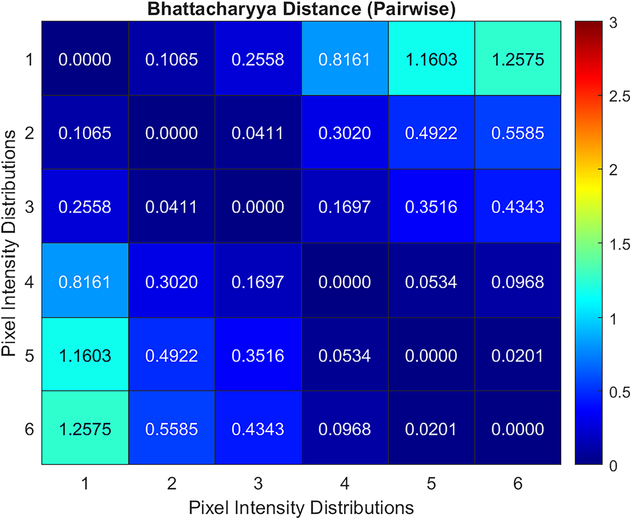
Figure 5: Heat map of the similarity between the pixel intensity distributions. Lower Bhattacharyya distance means higher similarity

As implied by Eq. (2), DCTGI is a pixel-based metric. Hence, to use it as an aggregate measurement to estimate chlorophyll, DCTGI must be converted to a single-value metric similar to SPAD measurements. The study used trimmed positive mean covering only 90% of the pixel-wise measurements. This step removes potential outliers by cutting the bottom and top 5% of values based on their percentile ranks, i.e., limiting the range to the 5th–95th percentile.

3.4 Phenotyping Using DCTGI

Phenotyping used in this study includes leaf counting, leaf area coverage, and chlorophyll content estimation. In an acquisition of the morphological traits of the coffee seedlings, DCTGI is used as a vegetation marker to isolate the leaves from the background. Fig. 6 summarizes the image processing steps to estimate the leaf count and coverage for each plant detected. The detected coffee seedling is cropped based on the region-of-interest (ROI) or the bounding box generated during detection. Then, DCTGI is calculated on the ROI, assuming that a seedling is correctly detected. A series of noise filtering algorithms identifies the largest object that represents the leaf coverage. Once computed, DCTGI can be rendered as a grayscale image. Median filtering reduces the salt-and-pepper noise in the grayscale image before binary conversion. Holes created during the binary conversion were flood-filled, while morphological opening removed the small structures. As expected, some non-plant segments remained in the image. These were removed by assuming that the largest segment (based on pixel count) corresponds to the actual plant. The largest segment provided the basis for calculating the leaf coverage area using the ground sampling distance (GSD). To compute the GSD, a 20 cm × 30 cm white marker is used as a reference for the ground equivalent of a pixel in centimeters Fig. 7. The computed GSD is 0.1 cm/px, which renders a pixel an equivalent ground area of 0.01 cm2. GSD calculation adopted the method used by Dadios et al. [32].

Figure 6: Image processing workflow to estimate the leaf count and coverage applied to the detected coffee seedling.

Figure 7: Computation of the Ground Sampling Distance (GSD) used a reference marker with known dimensions, which provides the equivalent ground distance (in centimeters) per pixel in the image. The GSD computed is 0.1 cm/px

Leaf area coverage is then determined by counting the pixels of the largest component and multiplying them by the equivalent ground area per pixel. On the other hand, the process determines the number of leaves by finding the distance of the pixels along the boundary to the centroid of the largest component. The distances are then plotted while maintaining the pixel sequence, creating a signal graph as shown in the output of the “boundary-centroid distance computation” block (refer to Fig. 6). By finding the peaks in the signal graph, the algorithm was able to determine the number of leaf apices.

Another use of the DCTGI values is for estimating the chlorophyll content without the SPAD meter. To determine the relationship of the DCTGI with the SPAD values, five regression polynomials were investigated, including linear, quadratic, cubic, exponential, and power functions. The SPAD meter used for measuring the chlorophyll contents includes nitrogen measurements. The regression models used actual measurements to identify the best fit for the DCTGI values calculated from the aerial images. Based on this relationship, phenotyping using the DCTGI provides the chlorophyll estimates from aerial images of the crops.

3.5 Validation

Because the experiment didn’t include tissue analysis to validate the accuracy of the chlorophyll and nitrogen estimates, the evaluation metrics used in this work only cover the agreement between the estimates derived from DCTGI calculations and those of the actual measurements using a SPAD meter. But for the other phenotyping traits, such as the leaf count and canopy cover, the estimates were validated by actual measurements of the plants and the aerial images.

4  Results and Discussion

4.1 Aerial Image Acquisition and SPAD Measurements

SPAD meters measure the leaf absorbances in the red and near-infrared regions. The SPAD value calculated from these absorbances is proportional to the amount of chlorophyll present in the leaf. The relative chlorophyll content (expressed in SPAD units) exhibited considerable variability among the sampled Liberica coffee seedlings. SPAD value ranges vary between crop types, but interpretation is relative to measurements from the same crop. In this study, using Liberica coffee seedlings as the primary specimen, the SPAD readings averaged 14.57 ± 9.24 units, indicating a wide variation in chlorophyll concentration. The median value (10.6434 SPAD units) is lower than the mean. This result suggests that most of the seedlings at the time of data collection have lower chlorophyll content, while a small subset exhibits significantly higher concentration. The minimum and maximum recorded SPAD values were 3.4699 and 43.0957, respectively, which suggests that leaf pigmentation is heterogeneous across the leaf samples. Similarly, the SPAD meter provides nitrogen estimates in mg/g. The nitrogen estimates displayed notable variation, with a mean of 7.4586% and a standard deviation of 3.0055%, reflecting moderate dispersion in nitrogen estimates across the sampled seedlings. The median nitrogen value (6.3406%) is slightly lower than the mean, again suggesting a right-skewed distribution. The nitrogen estimates ranged from 3.2901% to 16.2205%, further supporting the variability in nutrient availability and assimilation among the plants. Fig. 8 shows the distribution of the SPAD measurements of relative chlorophyll and nitrogen estimates. The chlorophyll distribution, depicted in the left histogram, is right-skewed, with a pronounced peak around 8 to 12 SPAD units, indicating that most samples have relatively low chlorophyll levels. A secondary, smaller peak appears around 18 to 22 SPAD units, suggesting a possible subpopulation within the dataset. The distribution exhibits a long tail extending beyond 30 SPAD units, indicating that while higher relative chlorophyll values are less frequent, they do occur in some instances. Similarly, the nitrogen distribution, shown in the right histogram, follows a right-skewed pattern with a primary peak around 5 to 7 mg/g. A secondary peak around 10 to 12 mg/g implies the presence of distinct groups within the data. The long tail extending beyond 12 mg/g suggests that although higher nitrogen values are uncommon, they are still present in the dataset. Both distributions agree that the majority of samples possess lower chlorophyll and nitrogen levels, with fewer instances of elevated concentrations.

Figure 8: Data distribution of chlorophyll and nitrogen content measurements from the SPAD meter

4.2 Detection of Coffee Seedlings from Aerial Images

Fig. 9 shows a sample detection, while Fig. 10 shows the performance of the coffee seedling detection model based on YOLO. The evaluation used two standard object detection metrics: average Intersection over Union (IoU) and average precision (AP) at a 0.5 IoU threshold (commonly referred to as mAP@0.5). The average IoU reflects the localization accuracy of the predicted bounding boxes of the seedlings relative to the labeled data. At the same time, the AP quantifies the detector’s ability to detect coffee seedlings across varying confidence thresholds correctly. The results achieved show a high average IoU and a moderately strong AP, and that it can reliably detect and localize coffee seedlings in aerial images with a good balance between precision and recall.

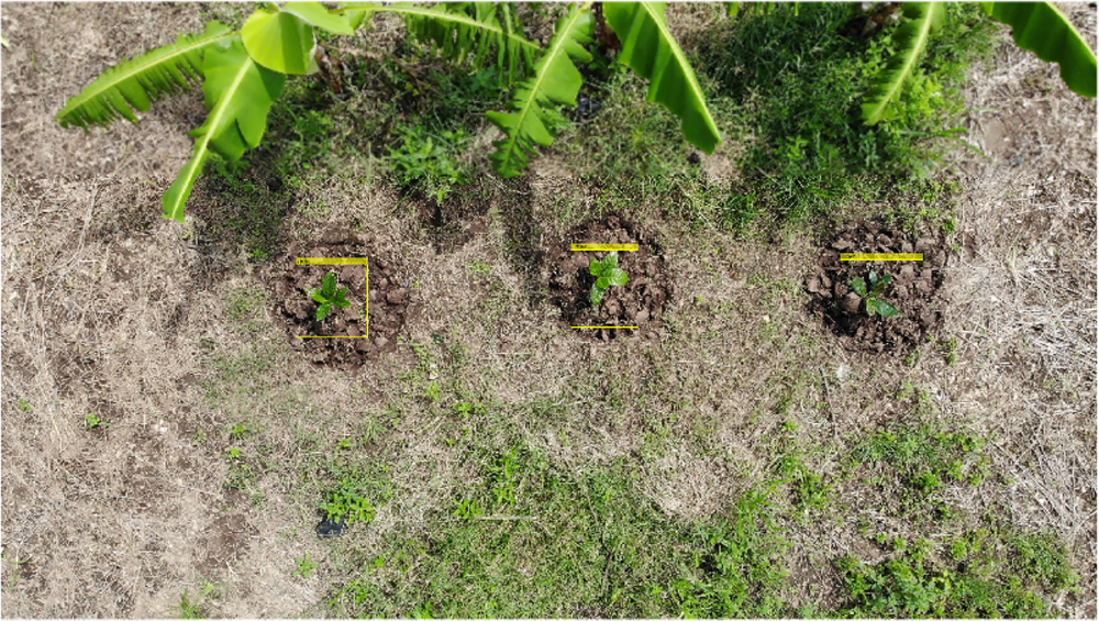
Figure 9: Result of the coffee seedling detection in aerial images

Figure 10: Result of the coffee seedling detection in aerial images

The coffee seedling image in RGB Fig. 11a serves as a reference for phenotyping because the image allows manual measurements of the growth metrics such as leaf count and canopy area. But extracting the leaves from the rest of the image requires enhancing the vegetative traits. The study employed DCTGI as a vegetation detection feature to separate the leaves from the rest of the image. Aside from that, the visualization provided in Fig. 11b offers a quantitative analysis of chlorophyll content estimate and overall vegetation health. However, the glare due to direct reflection of sunlight to the camera sometimes results in non-vegetation, which can be noticed by comparing the images in Fig. 11. The DCTGI aggregates values for the whole plant rather than individual pixels, which makes this level of accuracy acceptable.

Figure 11: Result of the plant detection is cropped images of the coffee seedlings (a). Then, from these cropped images, the DCTGI values are calculated. The visualization of the DCTGI values used in (b) shows red as high values and blue as minimal values

4.3 Correlation between DCTGI and SPAD Values

Table 2 shows the result of the regression models used to validate the assumption that the DCTGI values are associated with the SPAD measurements. The cubic model for the regression consistently outperforms the others in all three measures—R2, RMSE, and MAE, which implies a nonlinear relationship between DCTGI and SPAD measurements. Although some linearity occurs in the relationship because of the linear combination of reflectances in the equation of DCTGI, the results still show a positive regression, emphasizing that the greener the leaves are, the higher the DCTGI value is. Note, however, that a trimmed positive average of the DCTGI values in an image represents the whole plant.

Table 3 provides the correlation between chlorophyll content and the DCTGI. Note that the chlorophyll estimates here are derived from the SPAD measurements rather than from tissue analysis. The high Pearson correlation coefficient of r = 0.912533 indicates a strong positive linear relationship between these two variables, suggesting that DCTGI is a reliable predictor of chlorophyll content. This result is quite interesting because the regression analysis identified that the relationship is nonlinear. The relatively small standard deviation shows a narrower variability in DCTGI measurements, which may indicate more consistent readings for this parameter. The covariance value of 0.277444, while not easily interpretable on its own, further supports the positive relationship between chlorophyll content and DCTGI.

On the other hand, the results depicted in Table 4 show the nonlinearity of the relationship between the DCTGI and nitrogen measurements. However, this outcome occurs as expected because the SPAD meter derives nitrogen measurements from the same chlorophyll readings.

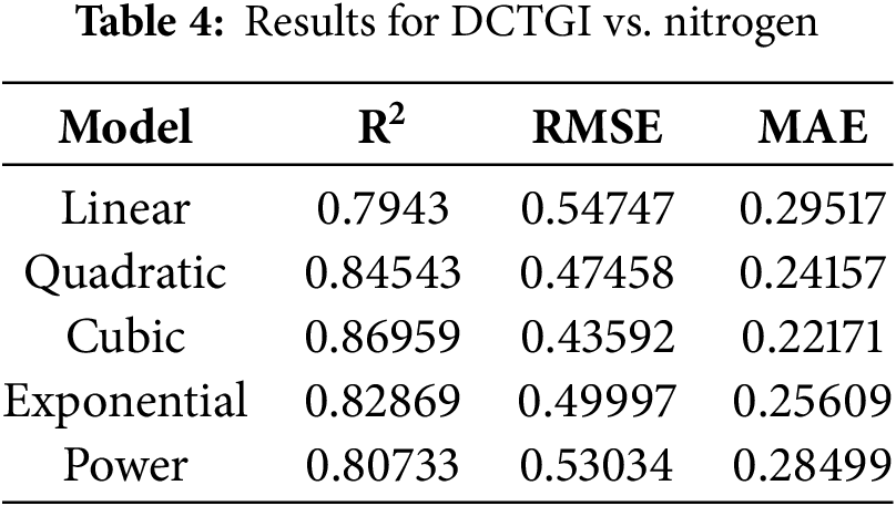
Fig. 12 presents the relationships of the DCTGI with chlorophyll and nitrogen measurements.

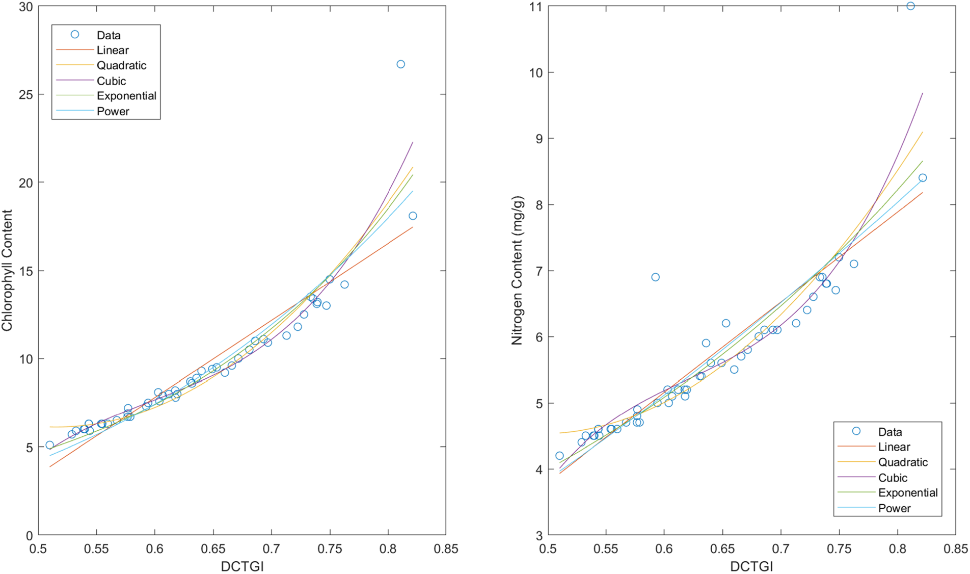
Figure 12: Regression models for estimating chlorophyll and nitrogen from DCTGI values

4.4 Comparison between Predicted and Actual Nitrogen Content Values

Figs. 13 and 14 present the agreement between the actual chlorophyll and nitrogen estimates derived from SPAD measurements and DCTGI, and shown from these plots that most of the pairs are within the limits of agreement (LOA), which indicates that the derived values agree with the actual measurements. However, the fact that there are still some measurements that do not agree with the derived values suggests that further studies where chlorophyll and nitrogen contents can be accurately measured (e.g., tissue analysis) are needed. Although some measurements are beyond LOA, the values are sparse and not concentrated in a specific range, suggesting a potential for random error.

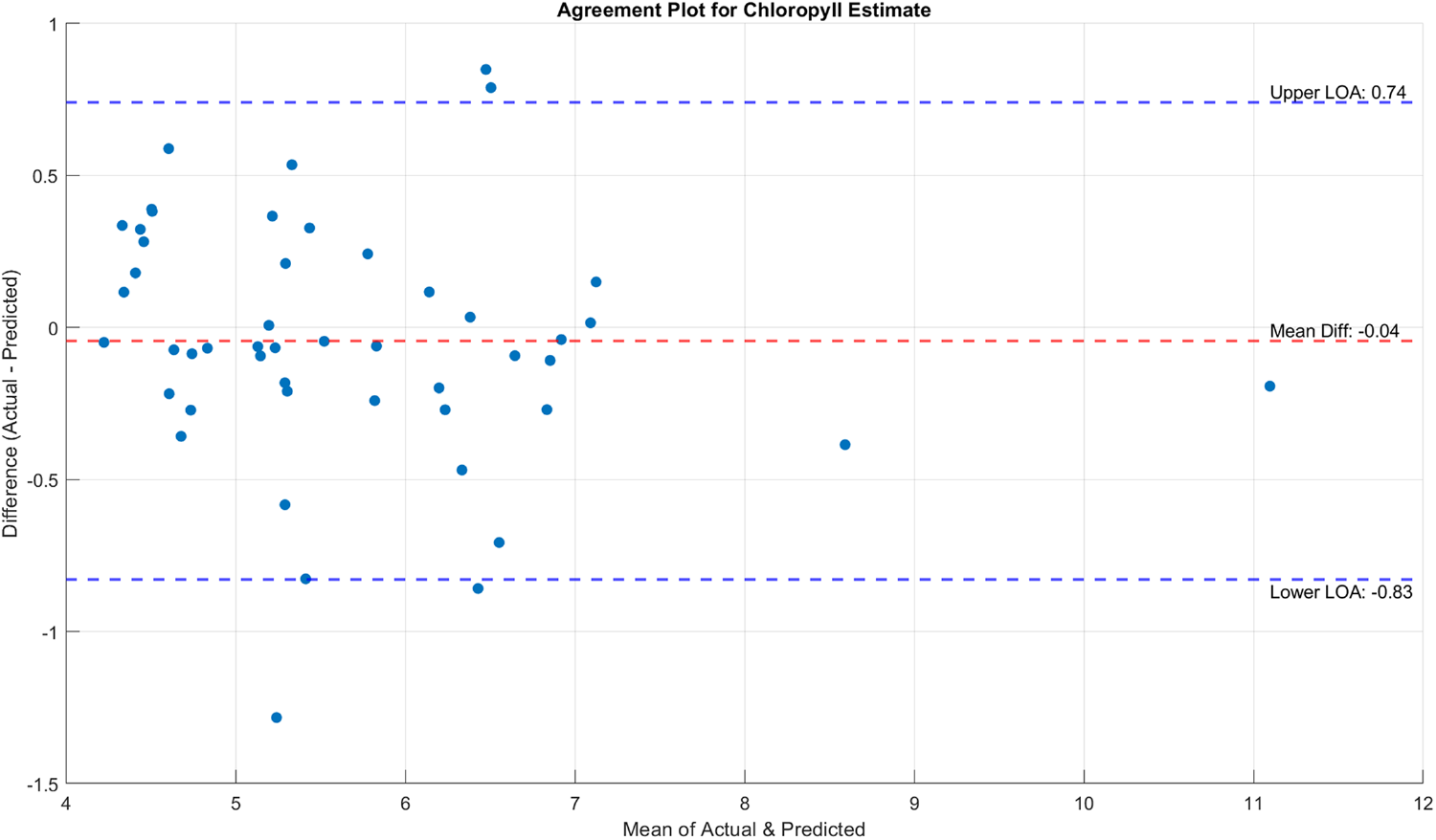
Figure 13: Difference between the estimated chlorophyll contents using DCTGI and the actual measurements using SPAD

Figure 14: Difference between the estimated nitrogen contents using DCTGI and the actual measurements using SPAD

4.5 Leaf Count and Coverage

The leaf counting algorithm demonstrated high accuracy and reliability across the evaluated dataset. Out of 50 samples, the majority of predictions matched the true leaf counts exactly. For the few mispredictions, the differences were minimal—typically within ±1 leaf—resulting in an average squared and percent errors of 0.36% and 3.31%, respectively. The mean percent error remained below 5%, which indicates that the algorithm maintains strong performance even when predictions are imperfect. Visual analysis further confirmed this, with correctly predicted values outnumbering incorrect ones, and deviations from ground truth being consistently minor. These results suggest that the algorithm is robust and well-suited for practical leaf counting tasks, offering precise estimations with minimal error in varying image conditions (Fig. 15). Similarly, the leaf cover estimates provide acceptable performance for having an average absolute percent error of almost 2% (Fig. 16).

Figure 15: Accuracy of leaf counting algorithm

Figure 16: Absolute error in % of leaf cover estimation

5  Conclusion

This study implemented aerial phenotyping by using VI derived from visible-spectrum imaging devices. The DCTGI showed a positive correlation with the chlorophyll and nitrogen measurements using the SPAD meter. The study supports a favorable consideration of RGB-based imaging devices for unmanned aerial systems, where the use of multispectral sensors can be a constraint. However, because the correlation between chlorophyll and nitrogen contents is inherent in the SPAD meter used and the values vary depending on the crops, there is a chance that the regression models will not be the same for other crops, which entails further studies. Nonetheless, the results gained from this work simplify the phenotyping tasks for Liberica coffee farms.

Despite the usefulness of the proposed approach in chlorophyll estimation of coffee seedlings, the current study lacks a temporal analysis on the progression of chlorophyll content from the transplanting of the coffee seedlings to the maturity of the plants. Further study may require additional data collection that may last for at least 5 years after transplanting. In addition, the current study can be extended to other crops to test the viability of the proposed approach in chlorophyll estimation, thereby opening opportunities to improve the DCTGI parameterization procedure for more flexible and robust applications.

Acknowledgement: The author thanks the student interns of the Digital Transformation Center for their assistance in data collection. The author also thanks Project BARAKO for the use of their Liberica Coffee Farm for this study.

Funding Statement: The author received no specific funding for this study.

Availability of Data and Materials: The data that support the findings of this study are available from the corresponding author, Anton Louise P. De Ocampo, upon reasonable request.

Ethics Approval: Not applicable.

Conflicts of Interest: The author declares no conflicts of interest to report regarding the present study.

References

1. Islam N, Rashid M, Pasandideh F, Ray B, Moore S, Kadel R. A review of applications and communication technologies for internet of things (IoT) and unmanned aerial vehicle (UAV) based sustainable smart farming. Sustainability. 2021;13(4):1821. doi:10.3390/su13041821. [Google Scholar] [CrossRef]

2. Ayaz M, Ammad-Uddin M, Sharif Z, Mansour A, Aggoune E. Internet-of-Things (IoT)-based smart agriculture: toward making the fields talk. IEEE Access. 2019;7:129551–83. doi:10.1109/ACCESS.2019.2932609. [Google Scholar] [CrossRef]

3. Olson D, Anderson J. Review on unmanned aerial vehicles, remote sensors, imagery processing, and their applications in agriculture. Agron J. 2021;113(2):971–92. doi: 10.1002/agj2.20595. [Google Scholar] [CrossRef]

4. Tariq M, Ahmed M, Iqbal P, Fatima Z, Ahmad S. Crop phenotyping. In: Systems modeling. Cham, Switzerland: Springer; 2020. p. 45–60. [Google Scholar]

5. Yang W, Feng H, Zhang X, Zhang J, Doonan J, Batchelor W, et al. Crop phenomics and high-throughput phenotyping: past decades, current challenges, and future perspectives. Mol Plant. 2020;13(2):187–214. doi:10.1016/j.molp.2020.01.008. [Google Scholar] [PubMed] [CrossRef]

6. Pérez-Bueno M, Pineda M, Barón M. Phenotyping plant responses to biotic stress by chlorophyll fluorescence imaging. Front Plant Sci. 2019;10:1135. doi:10.3389/fpls.2019.01135. [Google Scholar] [PubMed] [CrossRef]

7. Yeom J, Jung J, Chang A, Ashapure A, Maeda M, Maeda A, et al. Comparison of vegetation indices derived from UAV data for differentiation of tillage effects in agriculture. Remote Sens. 2019;11(13):1548. doi:10.3390/rs11131548. [Google Scholar] [CrossRef]

8. Deng L, Mao Z, Li X, Hu Z, Duan F, Yan Y. UAV-based multispectral remote sensing for precision agriculture: a comparison between different cameras. ISPRS J Photogramm Remote Sens. 2018;146:124–36. doi:10.1016/j.isprsjprs.2018.09.008. [Google Scholar] [CrossRef]

9. Gerhards M, Schlerf M, Mallick K, Udelhoven T. Challenges and future perspectives of multi-/hyperspectral thermal infrared remote sensing for crop water-stress detection: a review. Remote Sens. 2019;11(10):1240. doi:10.3390/rs11101240. [Google Scholar] [CrossRef]

10. Hunt ERJr, Daughtry CST, Eitel JUH, Long DS. Remote sensing leaf chlorophyll content using a visible band index. Agron J. 2011;103(4):1090–9. doi:10.2134/agronj2010.0395. [Google Scholar] [CrossRef]

11. De Ocampo ALP, Bandala AA, Dadios EP. Estimation of triangular greenness index for unknown peak wavelength sensitivity of CMOS-acquired crop images. In: Proceedings of the 2019 IEEE 11th International Conference on Humanoid, Nanotechnology, Information Technology, Communication and Control, Environment, and Management (HNICEM); 2019 Nov 29–Dec 1; Laoag, Philippines. p. 1–5. doi:10.1109/hnicem48295.2019.9072796. [Google Scholar] [CrossRef]

12. Bakirci M. Real-time vehicle detection using YOLOv8-nano for intelligent transportation systems. Traitement Signal. 2024;41(4):651–8. doi:10.18280/ts.410407. [Google Scholar] [CrossRef]

13. Ghanem ME, Marrou H, Sinclair TR. Physiological phenotyping of plants for crop improvement. Trends Plant Sci. 2015;20(3):139–44. doi:10.1016/j.tplants.2014.11.006. [Google Scholar] [PubMed] [CrossRef]

14. Tremblay N, Wang Z, Cerovic ZG. Sensing crop nitrogen status with fluorescence indicators: a review. Agron Sustain Develop. 2012;32(2):451–64. doi:10.1007/s13593-011-0041-1. [Google Scholar] [CrossRef]

15. Ali MM, Al-Ani A, Eamus D, Tan DKY. Leaf nitrogen determination using non—destructive techniques—a review. J Plant Nutr. 2017;40(7):928–53. doi:10.1080/01904167.2016.1143954. [Google Scholar] [CrossRef]

16. Zhang H, Wang L, Jin X, Bian L, Ge Y. High-throughput phenotyping of plant leaf morphological, physiological, and biochemical traits on multiple scales using optical sensing. Crop J. 2023;11(5):1303–18. doi:10.1016/j.cj.2023.04.014. [Google Scholar] [CrossRef]

17. Zhang B, Wu Y, Zhao B, Chanussot J, Hong D, Yao J, et al. Progress and challenges in intelligent remote sensing satellite systems. IEEE J Sel Top Appl Earth Obs Remote Sens. 2022;15:1814–22. doi:10.1109/JSTARS.2022.3148139. [Google Scholar] [CrossRef]

18. Angidi S, Madankar K, Tehseen MM, Bhatla A. Advanced high-throughput phenotyping techniques for managing abiotic stress in crops—a comprehensive review. Crops. 2025;5(2):8. doi:10.3390/crops5020008. [Google Scholar] [CrossRef]

19. Pettorelli N. The normalized difference vegetation index. New York, NY, USA: Oxford University Press; 2013. doi:10.1093/acprof:osobl/9780199693160.003.0002. [Google Scholar] [CrossRef]

20. Wang Y, Yang Z, Kootstra G, Khan H. The impact of variable illumination on vegetation indices and evaluation of illumination correction methods on chlorophyll content estimation using UAV imagery. Plant Methods. 2023;19(1):51. doi:10.1186/s13007-023-01037-7. [Google Scholar] [PubMed] [CrossRef]

21. Eitel J, Long D, Gessler P, Hunt EJr, Brown D. Sensitivity of ground-based remote sensing estimates of wheat chlorophyll content to variation in soil reflectance. Soil Sci Soc America J. 2009;73:1715–23. doi:10.2136/sssaj2008.0288. [Google Scholar] [CrossRef]

22. Dong T, Meng J, Shang J, Liu J, Wu B. Evaluation of chlorophyll-related vegetation indices using simulated Sentinel-2 data for estimation of crop fraction of absorbed photosynthetically active radiation. IEEE J Sel Top Appl Earth Obs Remote Sens. 2015;8(8):4049–59. doi:10.1109/jstars.2015.2400134. [Google Scholar] [CrossRef]

23. Mosslah AA, Abbas AH. An analysis of image processing in forestry and agriculture review. IOP Conf Ser Earth Environ Sci. 2023;1202(1):012003. doi:10.1088/1755-1315/1202/1/012003. [Google Scholar] [CrossRef]

24. Sun H. Crop vegetation indices. In: Encyclopedia of smart agriculture technologies. Cham, Switzerland: Springer; 2023. p. 1–7. doi:10.1007/978-3-030-89123-7_216-1. [Google Scholar] [CrossRef]

25. Zhang C, Filella I, Garbulsky MF, Peñuelas J. Affecting factors and recent improvements of the photochemical reflectance index (PRI) for remotely sensing foliar, canopy and ecosystemic radiation-use efficiencies. Remote Sens. 2016;8(9):677. doi:10.3390/rs8090677. [Google Scholar] [CrossRef]

26. Lemes EM, Coelho L, de Andrade SL, dos Santos Oliveira A, Marques MG, do Nascimento FMA, et al. Triangular greenness index to evaluate the effects of dicamba in soybean. AgriEngineering. 2022;4(3):758–69. doi:10.3390/agriengineering4030049. [Google Scholar] [CrossRef]

27. Polat N, Memduhoğlu A, Kaya Y. Triangular greenness index analysis for monitoring fungal disease in pine trees: a UAV-based approach. Bartın Orman Fak Derg. 2024;26(2):1–15. doi:10.24011/barofd.1352729. [Google Scholar] [CrossRef]

28. Starỳ K, Jelínek Z, Kumhálová J, Chyba J, Balážová K. Comparing RGB-based vegetation indices from UAV imageries to estimate hops canopy area. Agronomy Research. 2020;18(4):2592–601. doi:10.15159/ar.20.169. [Google Scholar] [CrossRef]

29. Redmon J, Farhadi A. YOLOv3: an Incremental Improvement. arXiv:1804.02767. 2018. [Google Scholar]

30. Hunt ERJr, Doraiswamy PC, McMurtrey JE, Daughtry CST, Perry EM, Akhmedov B. A visible band index for remote sensing leaf chlorophyll content at the canopy scale. Int J Appl Earth Obs Geoinf. 2013;21:103–12. doi:10.1016/j.jag.2012.07.020. [Google Scholar] [CrossRef]

31. Forero MG, Arias-Rubio C, González BT. Analytical comparison of histogram distance measures. In: Vera-Rodriguez R, Fierrez J, Morales A, editors. Progress in pattern recognition, image analysis, computer vision, and applications, CIARP 2018. Cham, Switzerland: Springer; 2019. p. 81–90. doi:10.1007/978-3-030-13469-3_10. [Google Scholar] [CrossRef]

32. De Ocampo A, Dadios E. Integrated weed estimation and pest damage detection in solanum melongena plantation via aerial vision-based proximal sensing. Philippine J Sci. 2021;150(3):1041–52. [Google Scholar]