Some Important Features of the Lambert Equivalent Azimuthal Projection

1  Introduction

Johann Heinrich Lambert (1728–1777) was a physicist, mathematician, astronomer and cartographer. His mathematical research included algebra, spherical trigonometry and perspective. He was the first to prove that π is an irrational number and the first to systematically use hyperbolic functions. His work on the theory of parallel lines is particularly significant. In his work Photometrie, he clearly distinguished the concepts of brightness and illumination, thus laying the foundations of photometry. In addition, he investigated the refraction of light in the atmosphere, then the paths of comets, and in this connection discovered new properties of conics. In his astronomical works, binary stars are mentioned for the first time [1,2].

According to Frischauf [3], the beginnings of the theory of mapping one surface onto another belong to Lambert, who dealt with the general problem of mapping a sphere and an ellipsoid onto a plane in the chapter Anmerkungen und Zusätze zur Entwerfung der Land und Himmelscharten (Notes and Additions to the Establishment of Maps of the Earth and Sky) printed in the third part of his Beyträge zum Gebrauche der Mathematik und deren Anwendung (Contributions to the Use of Mathematics and Its Application) [4].

Lambert was the first mathematician who dealt with the general properties of map projections. He considered the properties of conformality and equivalence and pointed to the fact that these two properties are mutually exclusive. In the aforementioned book, he published seven new map projections that he did not name, and today they are known as:

1.    Lambert Conformal Conic

2.    Transverse Mercator

3.    Lambert Azimuthal Equivalent

4.    Lagrange Projection

5.    Lambert Cylindrical Equivalent

6.    Transverse Cylindrical Equivalent

7.    Lambert Conic Equivalent

Let us also mention that the Lambertian function is defined as a mapping Lam:(0,π2)→R,

Lam(φ)=∫0φdxcos⁡x=12ln⁡1+sin⁡φ1−sin⁡φ=ln⁡tan⁡(π4+φ2)=sinh−1⁡(tan⁡φ)=tanh−1⁡(sin⁡φ)

This mapping appears in the equations of the normal Mercator projection [5,6].

In a previous paper [7], I researched points and lines on maps where the distortions are equal to zero. This is followed by examples of cylindrical, azimuthal, pseudocylindrical and a few other projections. These examples show that there need not be standard points at all, that there may be one or two standard points, as well as entire standard lines. In conclusion, I stated that in future research, other map projections should be included where the mathematical approach is somewhat more complex. These are, for example, the Aitoff, Hammer and Winkels Triple projection. The Hammer projection was created from the Lambert equivalent azimuthal projection. That is why it was necessary to first look for the distribution of linear distortions that occur during that projection, which is the topic of this article.

2  Azimuthal Projections

In normal azimuthal projections, images of meridians are lines that intersect at a single point at angles equal to the difference in their longitudes, and images of parallels are concentric circles centered at the intersection of the meridians. Accordingly, the general equations of normal azimuthal projections in polar coordinates can be written in this form

ρ=ρ(φ),δ=λ−λ0,(1)

where ρ is the radius of the parallel images, and δ is the angle between the meridian images. It is understood that only some uniformly distributed meridians are shown. φ denotes the latitude, λ is the longitude, and λ0 is the longitude of the central meridian of the area being mapped. The form of the function ρ=ρ(φ) depends on the mapping conditions, i.e., whether the projection is conformal, equivalent, equidistant, or has some other properties.

If a rectangular coordinate system x, y is set up so that its origin is at the center of the projection, then the rectangular coordinates in the right-handed (mathematical) coordinate system of each point in that projection are determined by the equations:

x=ρsin⁡δ,y=−ρcos⁡δ.(2)

We will arrive at the formulas for the local linear scale factors h along the meridian and k along the parallel from the general formulas by determining E and G from the projection equations (F=0) [8]:

E=(∂x∂φ)2+(∂y∂φ)2=(dρdφ)2(3)

G=(∂x∂λ)2+(∂y∂λ)2=ρ2.(4)

Azimuthal projections are most often used for small-scale maps, so we approximate the Earth with a sphere. For a sphere of radius R [8],

h=ER=−dρRdφ,(5)

k=GRcos⁡φ=ρRcos⁡φ.(6)

The minus sign in expression (5) is chosen because ρ=ρ(φ) is a decreasing function. The North and South Poles are not regular points of the geographical parameterization of the sphere. Therefore, all formulas in which the geographical latitude of the North or South Pole may appear should be understood as corresponding limit values.

The general formulas for normal azimuthal projections for the sphere are therefore

ρ=ρ(φ),δ=λ−λ0

x=ρsin⁡δ,y=−ρcos⁡δ

h=−dρRdφ,k=ρRcos⁡φ(7)

p=hk

sin⁡ω2=|h−k|h+k.

In Formula (7) φ∈[−π/2,π/2], λ∈[−π,π], the coordinate system x, y is mathematical, p is the local area scale factor, and ω is the maximum angle distortion. From Formula (7) it is evident that the distortions in the normal azimuthal projections depend only on the latitude φ, so the distortion isograms are circles that coincide with the projection of parallels.

Without loss of generality, we can assume that λ0=0 and R=1, so the projection equations will be slightly simplified and read:

x=ρ(φ)sin⁡λ,y=−ρ(φ)cos⁡λ,(8)

h=−dρdφ,k=ρcos⁡φ.(9)

3  Normal Lambert Equivalent Azimuthal Projection

3.1 Simple Case

Maps in the Lambert equivalent azimuthal projection are often used in normal aspect in atlases for maps of the polar regions, i.e., the northern and southern hemispheres. The transverse aspect is usually used for atlas maps of the eastern and western hemispheres. The oblique aspect is used for atlas maps of continents and oceans. The projection is recommended for maps of approximately circular areas that need to preserve the area [8].

In the simple normal aspect of this projection, the meridian images are straight lines that intersect in the image of the pole. The angles between the meridian images are equal to the angles between the meridians on the sphere. The parallel images are concentric circles. The distances between the parallel images gradually decrease with distance from the pole. In this projection, the entire sphere of the Earth can be shown (Fig. 1). The distortion is moderate in the image of a hemisphere but becomes very large on a map of the whole Earth (Fig. 2).

Figure 1: World map in the simple normal Lambert equivalent azimuthal projection

Figure 2: Distribution of linear distortions in the simple normal Lambert equivalent azimuthal projection, h blue, k red. The horizontal axis indicates degrees. The vertical axis indicates h and k, which are real numbers defined by (21). The yellow line is drawn at height 1

Let us derive the equations of the simple normal Lambert equivalent azimuthal projection. The equivalence condition in normal azimuthal projections of the sphere is expressed by the equation

p=hk=1,(10)

where h and k are local linear scale factors along the meridian and parallel [8]. Inserting the expression for the local linear scale factors (7) into (10) we obtain

−dρdφρcos⁡φ=1,(11)

from where

ρdρ=−cos⁡φdφ.(12)

By integrating, we get

ρ22=−sin⁡φ+K.(13)

If we set the condition that the North Pole is mapped as a point (for φ=π/2 it should be ρ=0), we get

K=1.(14)

By inserting this value into (13) we get

ρ2=2(1−sin⁡φ).(15)

This expression can also be written in the form

ρ2=4sin2⁡(π4−φ2),(16)

so it is finally

ρ=2sin⁡(π4−φ2).(17)

We chose the sign in (17) so that ρ≥0.

If we insert the obtained value for ρ into the expression for the local linear scale factor k (9), we obtain

k=2sin⁡(π4−φ2)cos⁡φ=1cos⁡(π4−φ2),(18)

and then

h=1k=cos⁡(π4−φ2).(19)

Therefore, the mapping equations and expressions for the local linear scale factors and distortion in simple normal equivalent azimuthal projections are:

ρ=2sin⁡(π4−φ2),x=ρsin⁡λ,y=−ρcos⁡λ(20)

h=cos⁡(π4−φ2),k=1h(21)

p=1,sin⁡ω2=|h−k|h+k.(22)

A map of the world in the simple normal equivalent azimuthal projection is shown in Fig. 1. From expression (20) we see that the images of all parallels are circles. If φ=π/2, then ρ=0, the north pole is mapped to a point. If φ=0, then ρ=2. The Equator is mapped into a circle of radius 2. If φ=−π/2, then ρ=2. The South Pole is mapped into a circle of radius 2 (Fig. 1).

For a point to be standard for a certain normal azimuthal projection, it is necessary and sufficient that at that point [7]

h=k=1.(23)

For the normal Lambert equivalent azimuthal projection (20), condition (23) reads:

cos⁡(π4−φ2)=1cos⁡(π4−φ2)=1,(24)

from which immediately follows the unique φ=π/2 from the interval [−π/2,π/2] and then ρ=0. So, in that projection, we have one standard point with the coordinates (x,y)=(0,0). The distribution of linear distortions is shown in Fig. 2.

If we set the condition that the North Pole is mapped not only as a point, but as a circle (Fig. 3), it follows from (13) (See also Section 3.3)

ρ=2(K−sin⁡φ),(25)

and in that case it should be

K≥1,(26)

so that the expression under the root is non-negative. From (25) it is easy to see that the North Pole will be mapped into a circle of radius 2(K−1), the Equator into a circle of radius 2K, and the South Pole into a circle of radius 2(K+1).

Figure 3: World map in the normal aspect of the general Lambert equivalent azimuthal projection, K=1.1

For the radius of the parallel images defined in (25), condition (23) gives

2(K−sin⁡φ)=cos⁡φ.(27)

After squaring, expression (27) can be written in the form

(sin⁡φ−1)2=2(1−K).(28)

Since the left side of (28) is always non-negative, and by assumption (26) and (28) will be fulfilled only for K=1. Therefore, the only simple normal azimuthal equivalent projection that has a standard point is the one for which K=1, i.e., the one for which Eq. (20) hold, which is the simple Lambert equivalent azimuthal projection.

3.2 “Tangent” and “Secant” Lambert Equivalent Azimuthal Projection

In the cartographic literature, tangent and secant projections are often mentioned. I am committed that the terms tangent and secant projection should be avoided in general, because they only make sense in perspective projections [9]. First, the derivation or definition of the Lambert equivalent azimuthal projection makes no mention of tangency or contact. The position of the projection plane in relation to the sphere being mapped is completely irrelevant. Furthermore, conclusions about an undistorted circle if a secant plane is used are a complete failure, because in the previous section we showed that an undistorted circle exists only for K=1, when the pole is mapped to a point.

The radius of the parallel corresponding to the latitude φ on the unit sphere is equal to cos⁡φ. In order for that parallel to be “secant” for the Lambert equivalent azimuthal projection, ρ(φ)=cos⁡φ should be valid, and this is the relation (27) that leads to the conclusion stated after Formula (28).

3.3 General Case

If K≥1, we have the most general case of the normal Lambert equivalent azimuthal projection (Eq. (25)). The North Pole will be mapped into a circle of radius 2(K−1) (Fig. 3). The local linear scale factor along meridians h will always be less than 1, while the local scale factor of linear along parallels k will be greater than 1 (Fig. 4). The blue and red lines in Fig. 4 nowhere reach the value 1. Thus, for K>1, there is no parallel for which h=1 or k=1 would hold, and especially h=k=1. In other words, for K>1 there is no parallel whose image in the Lambert equivalent azimuthal projection would be undistorted.

Figure 4: Distribution of linear distortions in the general normal Lambert equivalent azimuthal projection (K=1.1), h blue, k red. The horizontal axis indicates degrees. The vertical axis indicates h and k, which are real numbers defined by (21). The yellow line is drawn at height 1

If K>1, the entire world is depicted in a circular wreath. This general case of a normal Lambert equivalent azimuthal projection has not been investigated in the theory of map projections so far and seems to have no special practical value.

To conclude, it makes no sense to talk about tangent and secant projections in general, because the position of the projection plane is in no way connected to the sphere being mapped except for perspective projections. In addition, the introduction of the names tangent and secant can lead to wrong conclusions about the distribution of distortions.

It is commonly assumed that standard parallels and parallels that appear as the intersections of a developable surface and a sphere or ellipsoid coincide. In a previous paper [9], it has been shown that this is not true for azimuthal projections which are equidistant along meridians, equidistant along parallels (orthographic), or equivalent, because there is no standard parallel at all in such projections. Only some azimuthal conformal (stereographic) projections have a standard parallel, in which case it coincides with the secant parallel. Furthermore, there are azimuthal projections with two secant parallels and with infinitely many secant parallels. One can read more about this in Lapaine’s articles [9,10].

4  Transverse Lambert Equivalent Azimuthal Projection

4.1 Simple Case

In the transverse aspect, the central meridian is shown as a straight line. Meridians that are 90° from the central meridian form a circle. The images of the other meridians are complex curves that intersect at both poles. The distance between the images of the meridians decreases with distance from the central meridian. The image of the Equator is a straight line. The images of the other parallels are complex curves concave towards the nearer Pole. The distance between the images of the parallels decreases with distance from the Equator. Along the image of the meridian that is 90° from the central meridian, the parallels are placed at equal intervals (Fig. 5).

Figure 5: World map in the simple transverse Lambert equivalent azimuthal projection, λ0=45∘

Let us recall how the equations of the transverse Lambert projection are formally derived from the equations of the normal Lambert projection. First, Eq. (20) are written as follows:

ρ=2sin⁡(π4−φ′2),x′=ρsin⁡λ′,y′=−ρcos⁡λ′,(29)

and then a substitution is made:

cos⁡φ′cos⁡λ′=cos⁡φsin⁡λ

cos⁡φ′sin⁡λ′=sin⁡φ

sin⁡φ′=cos⁡φcos⁡λ.(30)

Substitution (30) is a special case of the general transition from the normal aspect of the projection to the transverse one:

cos⁡φ′cos⁡λ′=cos⁡φcos⁡(λ−λP)

cos⁡φ′sin⁡λ′=sin⁡φPcos⁡φsin⁡(λ−λP)+cos⁡φPsin⁡φ

sin⁡φ′=−cos⁡φPcos⁡φsin⁡(λ−λP)+sin⁡φPsin⁡φ,

which is Formula (10) in the article by Lapaine and Frančula [11]. When the values φP=0, λP=π/2 are taken for the coordinates of the new pole, expressions (30) are obtained. Let us first calculate

ρ=2sin⁡(π4−φ′2)=2(1−sin⁡φ′)=2(1−cos⁡φcos⁡λ),

sin⁡λ′=sin⁡φcos⁡φ′=sin⁡φ1−cos2⁡φcos2⁡λ,

cos⁡λ′=cos⁡φsin⁡λcos⁡φ′=cos⁡φsin⁡λ1−cos2⁡φcos2⁡λ,(31)

and then according to (29)

x′=2sin⁡φ1+cos⁡φcos⁡λ,y′=−2cos⁡φsin⁡λ1+cos⁡φcos⁡λ.(32)

To get a map with the cardinal points arranged as we are used to, i.e., North is up and South is down, it is necessary to rotate the image by 90°, i.e., apply the expressions

x=−y′,y=x′.(33)

In this way we get the equations of the simple transverse Lambert projection

x=2cos⁡φsin⁡λ1+cos⁡φcos⁡λ,y=2sin⁡φ1+cos⁡φcos⁡λ.(34)

Let us notice that the expression in the denominator in (34) can be equal to zero. Since φ and λ are geographical coordinates, this will happen if φ=0 and at the same time λ=π or λ=−π. We cannot map a point on the sphere whose coordinates are (φ,λ)=(0,π) or (φ,λ)=(0,−π) in the projection plane using Eq. (34). We will omit this point from further considerations.

With

cos⁡z=cos⁡φcos⁡λ(35)

Eq. (34) look a little simpler

x=21+cos⁡zcos⁡φsin⁡λ,y=21+cos⁡zsin⁡φ.(36)

Let us calculate

x2+y2=21−cos2⁡z1+cos⁡z=2(1−cos⁡z)≤4.

This means that a map of the entire world made in the projection to which Eq. (34) are applied will be placed in a circle of radius 2 (Fig. 5).

For φ=±π/2, cos⁡z=0, x2+y2=2, x=0, y=±2. So, the Poles are mapped to points.

For λ=±π/2, cos⁡z=0, x2+y2=2, we have the equation of a circle with its center at the origin and radius 2. The images of two meridians λ=±π/2 form a circle.

4.2 General Case

The considerations on the transverse Lambert equivalent azimuthal projection carried out in Section 4.1 are sufficient to achieve my goal, i.e., to apply it in further research on the Hammer projection. However, for the sake of completeness, let us briefly present the general case. If instead of the equation ρ=2(1−sin⁡φ)=2sin⁡(π4−φ2) when deriving the equations of the transverse Lambert equivalent azimuthal projection we start from the more general expression ρ=2(K−sin⁡φ) with K≥1, and apply the same procedure as in Section 4.1, we will obtain equations that can be written in the form

x=2(K−cos⁡z)1−cos2⁡zcos⁡φsin⁡λ,y=2(K−cos⁡z)1−cos2⁡zsin⁡φ.(37)

In the special case for K=1, Eq. (37) reduce to the already known (36). For K>1 we will obtain an image of a pseudopol in the form of a circle of radius 2(K−1) (Fig. 6). The entire world is depicted in a circular wreath. This general case of a transverse Lambert equivalent azimuthal projection has not been researched so far in the theory of map projections.

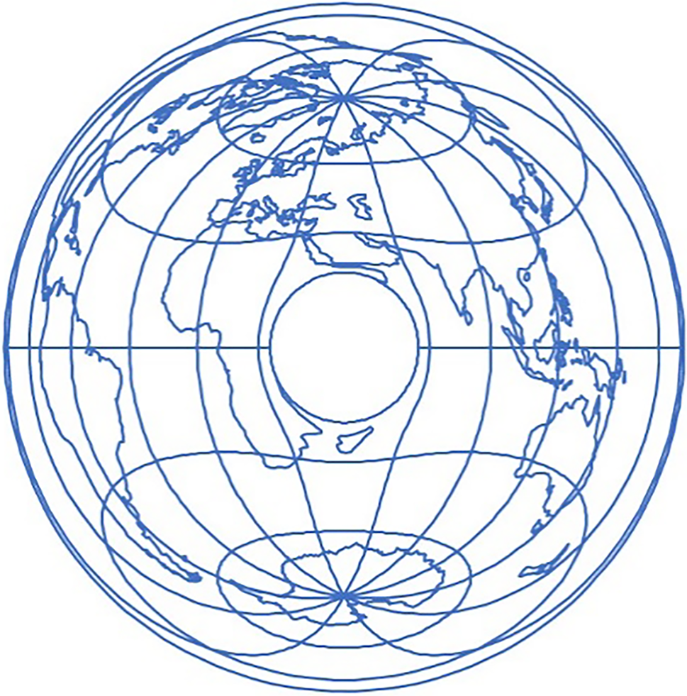
Figure 6: World map in the general transverse Lambert equivalent azimuthal projection, λ0=45∘, K=1.1

4.3 Partial Derivatives for the Simple Transverse Lambert Equivalent Azimuthal Projection

Partial derivatives are needed to estimate projection distortions. We will focus on the special case of the transverse Lambert equivalent azimuthal projection and Eq. (36), because we have seen the general case is not promising, while for further investigation of the Hammer projection only a simple form is needed. Let us do the math first:

∂∂φcos⁡z=−sin⁡φcos⁡λ,∂∂λcos⁡z=−cos⁡φsin⁡λ

∂∂φ1+cos⁡z=−sin⁡φcos⁡λ21+cos⁡z,∂∂λ1+cos⁡z=−cos⁡φsin⁡λ21+cos⁡z.(38)

After that, we can calculate the partial derivatives:

∂x∂λ=cos⁡φ2(1+cos⁡z)3[cos⁡λ(2+cos⁡z)+cos⁡φ](39)

∂x∂φ=−2sin⁡φsin⁡λ(1+cos⁡z)3(2+cos⁡z)(40)

∂y∂φ=12(1+cos⁡z)3[cos⁡λ+cos⁡φ(2+cos⁡z)](41)

∂y∂λ=sin⁡φcos⁡φsin⁡λ2(1+cos⁡z)3.(42)

4.4 Another Form of the Simple Transverse Lambert Equivalent Azimuthal Projection Equations and the Corresponding Partial Derivatives

Let us look for a different way to write the Lambert projection equations that would be more convenient for calculating partial derivatives. The following relation is known from trigonometry

1+cos⁡z=2cos2⁡z2.(43)

Using (43), the equations of the transverse Lambert equivalent azimuthal projection (36) can be written in the form

x=cos⁡φsin⁡λcos⁡z2,y=sin⁡φcos⁡z2,cos⁡z=cos⁡φcos⁡λ.(44)

The partial derivatives obtained based on expression (44) after rearrangement are:

∂x∂λ=cos⁡φcos⁡z2(cos⁡λ+cos⁡φsin2⁡λ4cos2⁡z2)(45)

∂x∂φ=−sin⁡φsin⁡λ2cos⁡z2(1+12cos2⁡z2)(46)

∂y∂φ=1cos⁡z2(cos⁡φ+sin2⁡φcos⁡λ4cos2⁡z2)(47)

∂y∂λ=sin⁡φcos⁡φsin⁡λ4cos3⁡z2.(48)

4.5 Third Form of the Simple Transverse Lambert Equivalent Azimuthal Projection Equations and the Corresponding Partial Derivatives

Following Solov’ev [12]:

x=2cos⁡φsin⁡λv,y=2sin⁡φv,v=1+cos⁡φcos⁡λ.(49)

The partial derivatives will be:

∂x∂λ=cos⁡φ2v(cos⁡λ+cos⁡φ+cos⁡λv2)(50)

∂x∂φ=−sin⁡φsin⁡λ2v(1+1v2)(51)

∂y∂φ=12v(cos⁡φ+cos⁡φ+cos⁡λv2)(52)

∂y∂λ=sin⁡φcos⁡φsin⁡λ2v3.(53)

Thus, we have three equivalent but different partial derivative notations for the simple Lambert equivalent azimuthal projection. Partial derivatives are needed to determine projection distortions. We will deal with this in the next section.

5  Standard Points in the Simple Transverse Lambert Equivalent Azimuthal Projection

At the end, let us investigate the places where the distortion is equal to zero in the simple transverse Lambert equivalent azimuthal projection. In a previous article [7], I derived the conditions that a single point must meet to be a standard point of a map projection. Assuming

∂y∂φ∂x∂λ−∂x∂φ∂y∂λ>0,(54)

these conditions are:

∂x∂λ=∂y∂φcos⁡φ,∂y∂λ=−∂x∂φcos⁡φ,(55)

and

(∂x∂φ)2+(∂y∂φ)2=1.(56)

In (54)–(56), x=x(φ,λ) and y=y(φ,λ) are functions that define the map projection, and φ∈[−π/2,π/2], λ∈[−π,π] are geographic coordinates. Conditions (55) mean that the point is mapped conformally, i.e., that Tissot’s indicatrix will be a circle. Condition (56) means that the radius of this circle will be 1.

Since for all equivalent projections

∂y∂φ∂x∂λ−∂x∂φ∂y∂λ=cos⁡φ,(57)

condition (54) will be fulfilled for all φ∈(−π/2,π/2). The poles are not regular points of the geographical parameterization of the sphere, so they should be considered separately.

In the previous sections, we introduced four equation sets of the Lambert transverse equivalent azimuthal projection. These were Eqs. (34), (36), (44) and (49). For all these equations, we calculated partial derivatives. Among them, we choose those with which we can most easily verify conditions (55) and (56). With a little analysis, it can be determined that for this purpose Eqs. (50)–(53) will be the most convenient to use.

If λ=0, then

v=1+cos⁡φ=2cos⁡φ2(58)

∂x∂λ=cos⁡φcos⁡φ2,∂x∂φ=0,∂y∂λ=0,∂y∂φ=cos⁡φ2.(59)

If we insert the partial derivatives (59) into (55) we get

cos⁡φcos⁡φ2=cos⁡φ2cos⁡φand0=0.(60)

With the assumption φ≠±π/2, from (60) we get cos⁡φ2=1 and from there φ=0. Relation (56) is fulfilled for φ=0. Accordingly, we have a standard point (φ,λ)=(0,0), i.e., (x,y)=(0,0). We have obtained one standard point, but how do we know that there are no more such points? To answer that question, let us include the partial derivatives (50)–(53) in (55). If we insert partial derivatives into

∂x∂λ=∂y∂φcos⁡φ,

we get

cos⁡φ2v[cos⁡λ+cos⁡φ+cos⁡λv2]=cos⁡φ2v[cos⁡φ+cos⁡φ+cos⁡λv2],(61)

from which it is immediately clear that cos⁡λ=cos⁡φ must hold true. If we substitute the partial derivatives in

∂y∂λ=−∂x∂φcos⁡φ,and considering cos⁡λ=cos⁡φ, we will obtain that the only solution is φ=λ=0, that is, there is only one standard point (φ,λ)=(0,0), or (x,y)=(0,0). Therefore, apart from the standard point (φ,λ)=(0,0) in the simple Lambert transverse equivalent azimuthal projection, there are no other standard points.

5.1 A Simpler Way to Determine the Standard Point in the Simple Transverse Lambert Equivalent Azimuthal Projection

Since the equations of the Lambert transverse equivalent azimuthal projection can be written in the form (21), which is formally equal to the form (18), then for the Lambert transverse equivalent azimuthal projection we can write the local linear scale factors according to the model of the normal projection.

h=cos⁡(π4−φ′2),k=1cos⁡(π4−φ′2)=1h(62)

and conclude that (19) will hold for the transverse Lambert equivalent azimuthal projection if

cos⁡(π4−φ′2)=1cos⁡(π4−φ′2)(63)

holds. From there, φ′=π/2 and then ρ=0 immediately follows. So, in that projection, we have one standard point with the coordinates (x,y)=(0,0). The distribution of linear distortions is identical to the distribution of distortions of the normal simple Lambert equivalent azimuthal projection (Fig. 2).

5.2 The Simplest Way to Determine the Standard Point in the Simple Transverse Lambert Equivalent Azimuthal Projection

A third, even simpler method without additional calculations would be to apply the property of map projections according to which all aspects of a projection (normal, oblique and transverse) have the same distribution of distortions.

Transverse and oblique projections are created by reparametrization from normal aspect projections. Since the first differential form is invariant to the change of parameters [13,14], the distortion distribution will not change with the transition from normal to transverse or oblique projection. Since the normal simple Lambert equivalent azimuthal projection (20) has only one standard point located at the origin of the coordinate system, then this is also true for the transverse aspect of this projection.

6  Conclusion

The Lambert equivalent azimuthal projection is one of the seven map projections proposed by J. H. Lambert. Although it was invented many years ago, this projection is still relevant today [15–20]. Scientists publish articles about it in journals [21,22], and future scientists study it as part of their doctoral dissertations [23].

This projection is often used in the normal aspect in atlases for maps of the polar regions. The transverse aspect is commonly used for Eastern and Western Hemisphere atlas maps. When researching that projection, it was observed that the general case of a normal and transverse Lambert equivalent azimuthal projection is not yet known in the theory of map projections. That is why the Lambert equivalent azimuthal projection was divided into a simple and a general form. Since the general case does not look promising in applications, and further research on the Hammer projection requires the simple case, it was investigated in more detail.

The equations of the simple transverse aspect can be written in several ways. Among several forms of the equations of the transverse aspect of the projection, I chose the form that is most adept at calculating the partial derivatives, which are necessary for the determination of distortions. The article presents the distribution of the local linear scale factor along the (pseudo) meridians and (pseudo) parallels and found that there is only one point where the distortion is zero.

Given that the Hammer projection was created from the simple transverse Lambert equivalent azimuthal projection, the research conducted and the results obtained can be used in future research on the Hammer projection.

Acknowledgement: Not applicable.

Funding Statement: The author received no specific funding for this study.

Availability of Data and Materials: Not applicable.

Ethics Approval: Not applicable.

Conflicts of Interest: The author declares that he has no conflicts of interest to report regarding the present study.

References

1. Bollmann J, Koch WG. Lexikon der kartographie und geomatik. Berlin/Heidelberg, Germany: Spektrum Akademischer Verlag; 2001. (In German). [Google Scholar]

2. Hrvatska E, Lambert JH. Miroslav krleža lexicographic institute. [cited 2024 Apr 1]. (In Croatian). Available from: http://www.enciklopedija.hr/Natuknica.aspx?ID=35243. [Google Scholar]

3. Frischauf J. Die abbildungslehre und deren anwendung auf kartographie und geodäsie. Teubner, Leipzig: Druck und Verlag von B.G; 1905. (In German). [Google Scholar]

4. Lambert JH. 6th Chapter: Anmerkungen und Zusätze zur Entwerfung der Land- und Himmelscharten [Notes and comments on the composition of terrestrial and celestial maps]. In: Beyträge zum gebrauche der mathematik und deren anwendung. dritter theil Berlin: Verlag der Buchhandlung der Realschule; 1772. (In German). [Google Scholar]

5. Lee LP. Conformal projections based on elliptic functions. Cartographica, Monograph no. 16, supplement no. 1 to Canadian Cartographer. 1976. Vol. 13, 128 p. [Google Scholar]

6. Rickey VF, Tuchinsky PM. An application of geography to mathematics: history of the integral of the secant. Math Mag. 1980;53(3):162–6. doi:10.1080/0025570x.1980.11976846. [Google Scholar] [CrossRef]

7. Lapaine M. Standard points and lines in map projections. KN-J Cartogr Geogr Inf. 2024;74(2):159–67. doi:10.1007/s42489-024-00168-8. [Google Scholar] [CrossRef]

8. Snyder JP. Map projections—a working manual. Washington, DC, USA: U.S. Government Printing Office; 1987. 383 p. Reprinted 1989 and 1994 with corrections. [Google Scholar]

9. Lapaine M. Standard parallel and secant parallel in azimuthal projections. Cartogr Geoinf. 2017;16(28):72–88. [Google Scholar]

10. Lapaine M. Sekushchie paralleli v azimutal’nyh proektsiyah [Secant Parallels in Azimuthal Projections]. Geod Cartogr. 2019;80(4):39–54. (In Russian). doi:10.22389/0016-7126-2019-946-4-39-54. [Google Scholar] [CrossRef]

11. Lapaine M, Frančula N. Map projection aspects. Int J Cartogr. 2016;2(1):38–58. doi:10.1080/23729333.2016.1184554. [Google Scholar] [CrossRef]

12. Solov’ev MD. Matematicheskaya kartografiya. Moscow, Russia: Nedra; 1969. 286 p. (In Russian). [Google Scholar]

13. Pressley A. Curvature of surfaces. In: Elementary differential geometry. London, UK: Springer; 2001. p. 123–45. doi:10.1007/978-1-4471-3696-5_6. [Google Scholar] [CrossRef]

14. Jia Y-B. Surface curves and fundamental forms (Com S 477/577 Notes). [cited 2020 Nov 11]. Available from: https://faculty.sites.iastate.edu/jia/files/inline-files/surface-curves.pdf. [Google Scholar]

15. Wikipedia. Lambert azimuthal equal-area projection. [cited 2025 Apr 10]. Available from: https://en.wikipedia.org/wiki/Lambert_azimuthal_equal-area_projection. [Google Scholar]

16. ArcGIS Pro. Lambert azimuthal equal-area. [cited 2025 Apr 10]. Available from: https://pro.arcgis.com/en/pro-app/latest/help/mapping/properties/lambert-azimuthal-equal-area.htm. [Google Scholar]

17. Wolfram Math World. Lambert Azimuthal equal-area projection. [cited 2025 Apr 10]. Available from: https://mathworld.wolfram.com/LambertAzimuthalEqual-AreaProjection.html. [Google Scholar]

18. GMT Community Forum. Azimuthal Lambert. [cited 2025 Apr 10]. Available from: https://www.pygmt.org/latest/projections/azim/azim_lambert.html. [Google Scholar]

19. PROJ. LAEA. [cited 2025 Apr 10]. Available from: https://proj.org/en/stable/operations/projections/laea.Html. [Google Scholar]

20. GMT Map Projections—GMT 6.6.0 Documentation. Azimuthal projections. [cited 2025 Apr 10]. Available from: https://docs.generic-mapping-tools.org/latest/reference/map-projections.html#azimuthal-projections. [Google Scholar]

21. Öztürk E. Lambert azimuthal equal-area projection. Eskişehir Tech Univ J Sci Technol A. 2024;25(3):380–9. doi:10.18038/estubtda.1410864. [Google Scholar] [CrossRef]

22. Kerkovits K. Development of a low-distortion authalic sphere for the oblique azimuthal equal-area map projection of the spheroid. J Spat Inf Sci. 2025;2025(30):117–29. doi:10.5311/josis.2025.30.402. [Google Scholar] [CrossRef]

23. Gilić F. Development of a geospatial data model for global land cover data storage and handling [Ph.D. thesis]. Zagreb, Croatia: University of Zagreb Faculty of Geodesy; 2025. [Google Scholar]