Predicting Soil Carbon Pools in Central Iran Using Random Forest: Drivers and Uncertainty Analysis

1  Introduction

As the most significant carbon resource on Earth, the soil serves a fundamental function in carbon sequestration and global climate change [1,2]. Soil organic carbon (SOC) and soil inorganic carbon (SIC) can control the largest territorial carbon storage. Globally, the estimated storage inventory of SOC in the one-meter depth varies from 1200 to 1600 picograms, while the inventory of SIC has been assessed as 695 to 1738 Pg for a similar depth [3]. SOC storage is much higher than SIC in surface soils. Nowadays, human activities, particularly the development of industries, deforestation, and the use of fossil fuels can increase carbon dioxide and extra greenhouse gas concentrations in the air, leading to global warming concerns. SOC stocks represent the largest terrestrial carbon pool and play a critical role in climate change mitigation.

Globally, SOC can be regarded as a noteworthy factor for modeling greenhouse gas transpiration in different climate change scenarios. SOC content is closely dependent on land use/cover and environmental factors, which include geology, drainage, topography, climate, and intrinsic soil properties, as well as anthropogenic activities [4–6]. Even a low change of the content owing to management practices in a relatively large region could result in considerable emission of CO2 as well as carbon cycling changes in Earth’s ecosystems. SOC content can be regarded as a serious parameter in the assessment of soil quality [7]. Furthermore, it can improve soil aggregation [8], hamper soil loss, decrease land vulnerability, enhance the nutrient cycle and its availability, and increase water storage capacity [9].

Batjes [7] and Marchant et al. [8] indicated that about 33% of the worldwide C stocks that are agglomerated in the soil’s upper meter had some inorganic compounds. SIC, which mainly consists of carbonates, provides important information on mineralogy and soil chemical functions involving pH and exchangeable cations that are essential for plant growth [9]. Conditions with enough soil moisture encourage the build-up of SOC and frequently have low SIC. Arid and semi-arid areas with limited biomass output may have SIC-rich soils with little SOC buildup [10]. Therefore, these findings imply that SOC and SIC may have an offsetting impact.

Field surveys for enlightening SOC and SIC resources are accurate; nevertheless, they are expensive and time-consuming, as well as labor-intensive [2]. The variation of soil characteristics had been previously attained from some spatial approaches including such deterministic approaches as the nearest neighbor approach and inverse distance weighting (IDW), additionally, stochastic approaches like universal simple kriging and ordinary [11]. Afterward, there was the introduction of hybrid methods by conjoining deterministic and stochastic approaches [4]. Digital soil mapping (DSM) and effective machine learning models (ML) have been extensively employed recently for surveying and geographic estimation of soil parameters utilizing a variety of environmental variables [5,12].

Remote sensing techniques can be regarded as a necessary part of DSM [6]. Environmental variables that are frequently used to predict soil-forming components might be either qualitative or quantitative. The primary predictors significant for estimating soil properties are typically the environmental variables obtained from the digital elevation model (DEM) and its derivatives, remote sensing indices, and thematic maps (legacy geology, land use, geomorphology, and legacy soil units) [12]. In addition, environmental variables may be classified into passive or static (i.e., geology, legacy soil map) and active or dynamic (i.e., climatic) variables [13]. Environmental variables that reflect the impacts of organisms including vegetation, land cover, and land use maps have been applied for predicting SOC by DSM [5].

There is a variety of machine learning models in DSM to get the spatial associations existing among soil properties and environmental factors; this is subsequently followed by the target soil attributes’ spatial variability. There has been an assessment of many machine learning algorithms for predicting some soil characteristics (i.e, Cubist, artificial neural networks, multiple linear regression, k-nearest neighbors, partial least squares regression, multinomial logistic regression, random forest, support vector machine, and genetic algorithms [14].

Zeraatpisheh et al. [12], aiming to improve SOC spatial prediction by applying the environmental variables selection method, used a wide range of machine learning algorithms comprising RF, Cu, SVM, and PLSR, showing that Cu could be regarded as the most powerful in commonly used variables (topographic properties as well as single-time remote sensing data); meanwhile, RF was more powerful when used remote sensing time-series data. In another study, Naimi et al. [15] examined the data by 5 MLs of RF, k-nearest neighbors (KNN), SVM, PLSR, artificial neural networks, and the individual models ensemble.

Arid as well as semi-arid regions account for more than 85% of Iran [15], understanding SOC and SIC storage and their contributions can be very important for decision-makers and governors. Moreover, knowledge about the stock of these two components is very crucial regarding carbon sequestration and global warming. Furthermore, it is very vital to identify the controlling factors of these two target variables. The selected watershed, located in central Iran, is characterized by low annual precipitation and high evapotranspiration, sparse vegetation cover, and heterogeneous soil types. These arid to semi-arid conditions pose serious constraints on organic matter accumulation, leading to naturally low SOC and high SIC concentrations. Human-induced pressures such as overgrazing, inappropriate land use, and limited water availability exacerbate soil degradation and carbon loss. This ecological sensitivity makes the area a strategic testbed for evaluating predictive models and identifying key environmental drivers of carbon variability in semi-arid systems.

Our research involved analyzing the relationship between SOC and SIC and different datasets (like land use, geology, and geomorphology) independently. We also assessed the impact of incorporating or excluding satellite imagery on model performance using machine learning techniques. Consequently, this study attempted (i) to assess SOC and SIC prediction at the watershed basin using environmental variables, and (ii) variable importance analysis (via) and partial dependence plots (PDP) analysis were considered to find the major factors in controlling SOC and SIC variability at the given watershed, in the center of Iran.

2  Materials and Methods

2.1 Description of the Study Area

The study area was located in the western parts of Isfahan Province, in the center of Iran (Fig. 1). The average elevation of the study area is 2380 m a.s.l with a mean slope of 3.3% [16]. The region receives an average annual precipitation of 324.3 mm and has a mean annual temperature of 9.8°C. Conferring to the Koppen organization, the climate can be ordered as semi-arid, with chilly winters. The chosen area is a part of the Sanandaj-Sirjan zone geologically. According to [17], the most common rocks are Quaternary deposits, shale, limestone, and slate. In the area under investigation, pasture, dryland agriculture, and irrigated farming are the most common land uses (Fig. 2).

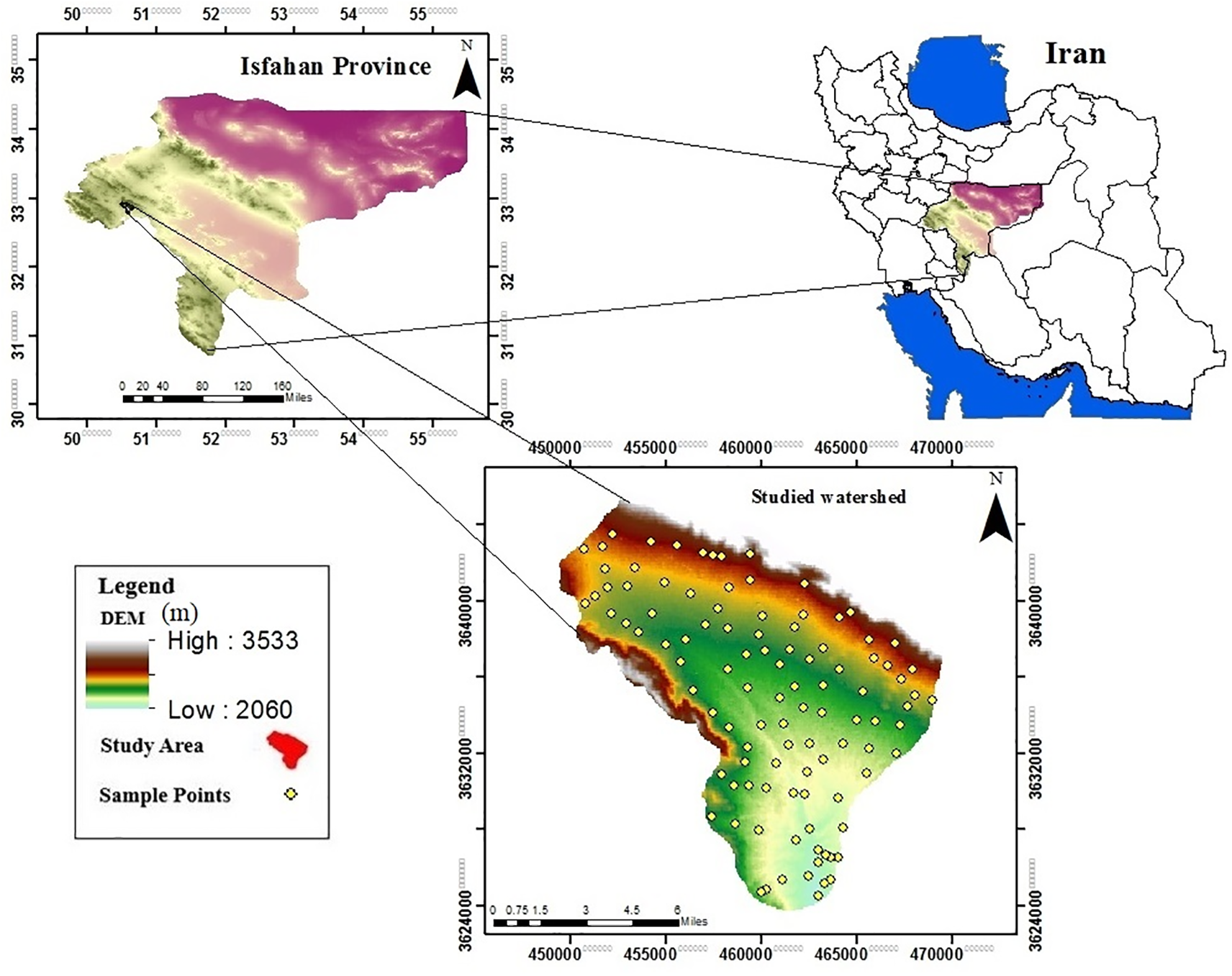
Figure 1: The study area is located in Isfahan province, the center of Iran, and the spatial distribution of sampling points is illustrated on the digital elevation model of the selected watershed

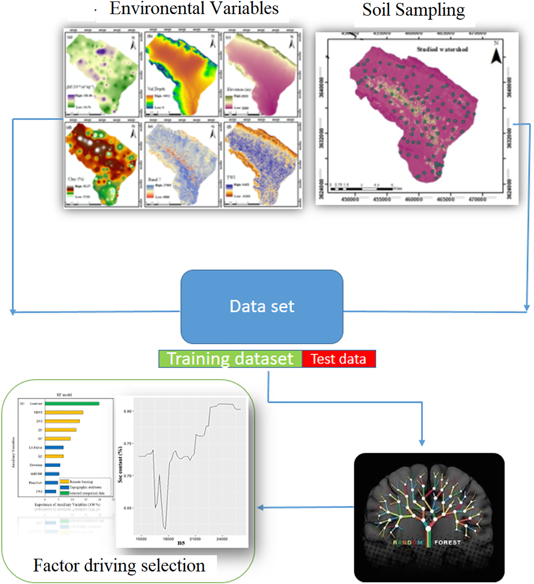
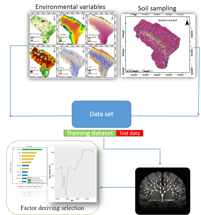
Figure 2: The overall research workflow

2.2 Field and Laboratory Studies

For the current investigation, 100 points were selected for taking soil samples in the summer of 2021 using the random sampling approach (Fig. 1). GPS was employed to capture the sampling spatial points during the process (Fig. 1). Five cores from 0 to 20 cm of topsoil were collected for each sampling point, completing a square’s corners to create a sort of composite sample. Every single one of these samples was allowed to air dry at ambient temperature. After that, impurities were removed. In the end, the samples under consideration were run through a 2 mm sieve so as to facilitate laboratory examination [18]. Analysis of SOC was done by the wet oxidation approach proposed by Nelson and Sommers (1982). Calculation of SIC content was done as 0.12× calcium carbonate equivalent [19]. Bernard’s calcimeter method was used for measuring the soil carbonate content [19].

2.3 Environmental Variables

In the present study, four datasets including topographic attributes extracted from DEM, remote sensing data, climatic layers, and categorical data such as land use and geomorphology maps were used as SOC and SIC driving forces (Table 1). The RS dataset included vegetation indices: Landsat 8 images from August to September of 2021 that coincided with the period of soil survey and sampling collection with less than 10% cloud cover were acquired from the USGS database (Table 1).

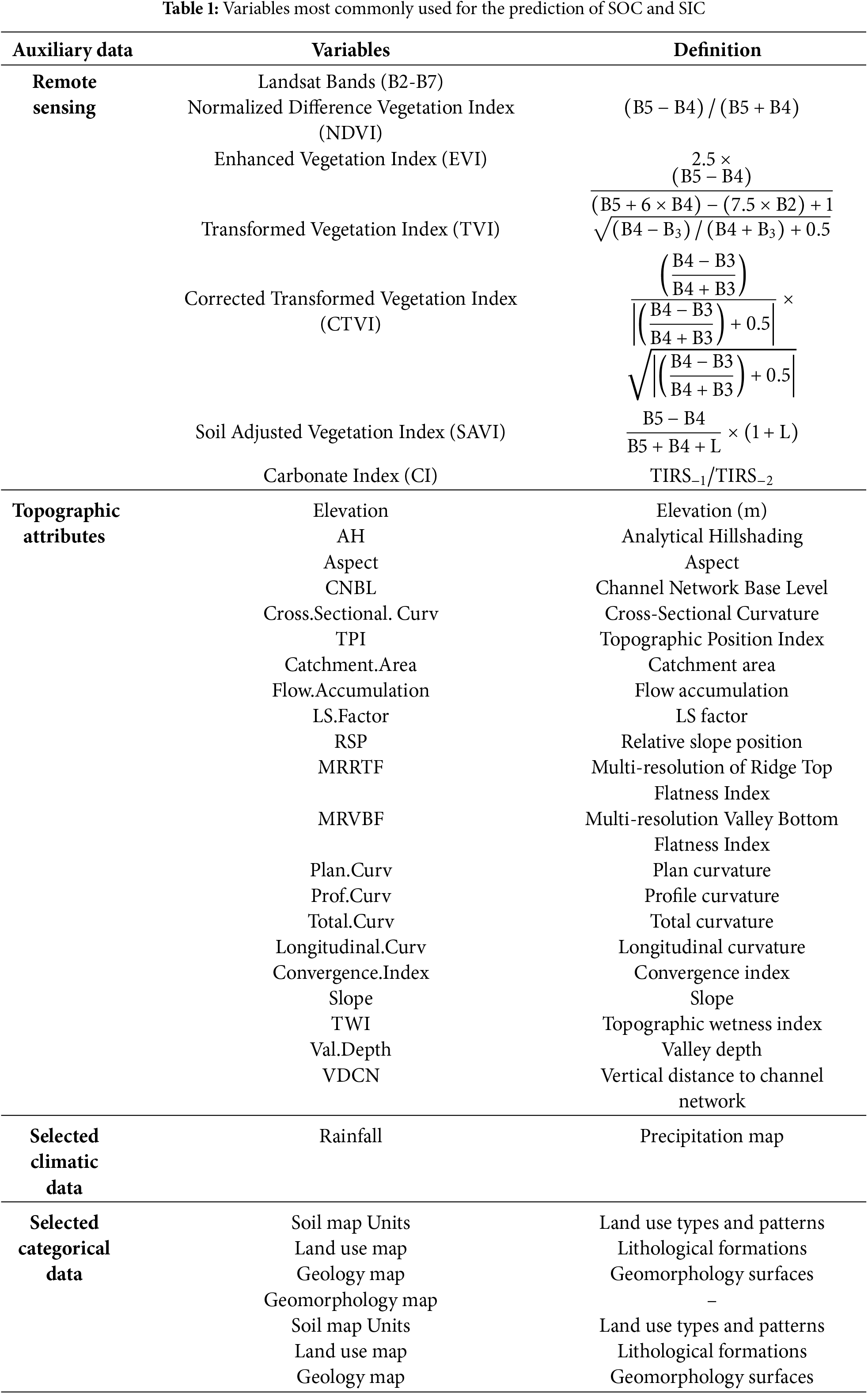
Topography can be considered as one of the foremost soil-forming factors in arid and semi-arid regions [12]. Therefore, the Aster GDEM database was used to get a digital elevation model (DEM) with 30 m × 30 m cell sizes, and some topographic attributes described in Table 1 were calculated [20]. The SAGA GIS software (version 4.7) was used to extract RS and topographic attributes [21].

The mean monthly precipitation for the period from 1997 to 2018 was obtained from the Meteorological Organization of Iran (IRIMO). A precipitation interpolated map was then spatialized by using the Inverse Distance Weighted (IDW) method in ArcMap 10.5 [21,22]; finally, the relevant precipitation map was applied as a designated climatic data (Table 1).

Land cover, legacy soil map units, geology, and geomorphology maps were used in this research as categorical variables (Table 1). Landsat 8 images were obtained on 3 September 2020, and ENVI 5.3 software was applied to prepare the land cover map. One of the input variables included a land use map that is presented in Fig. 3a, and the dominant land cover components are residential areas (7.70 km2), rainfed farmlands (83.65 km2), rangelands (60.03 km2) and irrigated agricultural lands (36.74 km2).

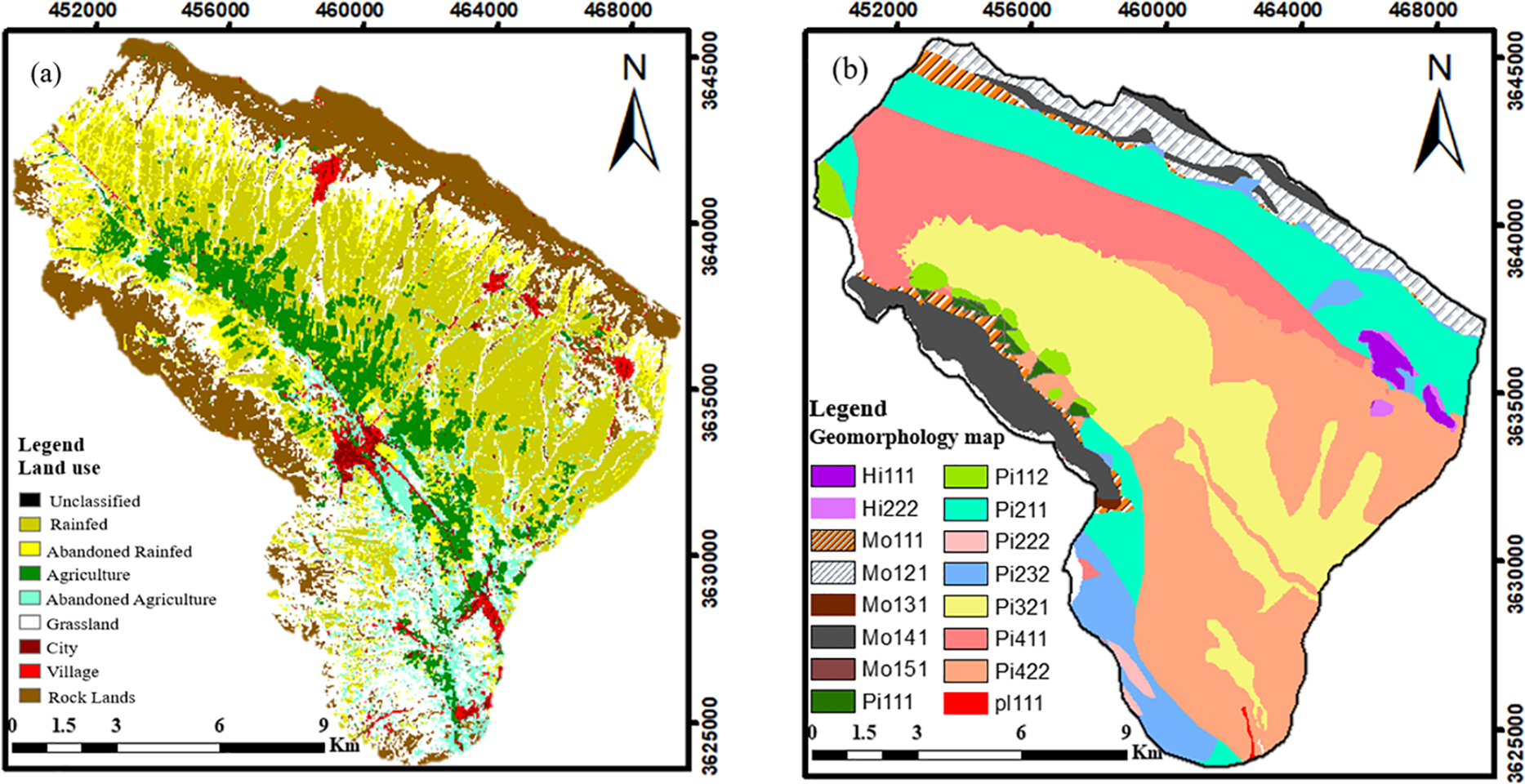
Figure 3: Land use (a) and geomorphology map (b) of the study area in Isfahan Province. Codes referring to geomorphic surfaces can be seen in Table 2

The geomorphology map was generated using Google Earth imagery as a base. Landscape positions, geology, slope, aspect, and landforms were considered to delineate distinct geomorphic units. To capture the complexity of the terrain, a four-level geomorphic hierarchy was adopted, encompassing landscapes, landforms, lithology, and geomorphological surfaces [22]. Ultimately, sixteen geomorphic components were identified and mapped (Fig. 3b, Table 2).

Fig. 4 presents additional variables (such as Elevation, Slope, Valley Depth, Band 2 Landsat 8, Band 7, and Normalized Difference Vegetation Index), incorporated into the subsequent soil organic carbon (SOC) and soil inorganic carbon (SIC) prediction models. To ensure consistency across platforms, all spatial datasets were standardized to the WGS 1984 coordinate system and projected using the Universal Transverse Mercator (UTM) Zone 32N. This standardization minimized spatial discrepancies and ensured accurate overlay and analysis across different software environments.

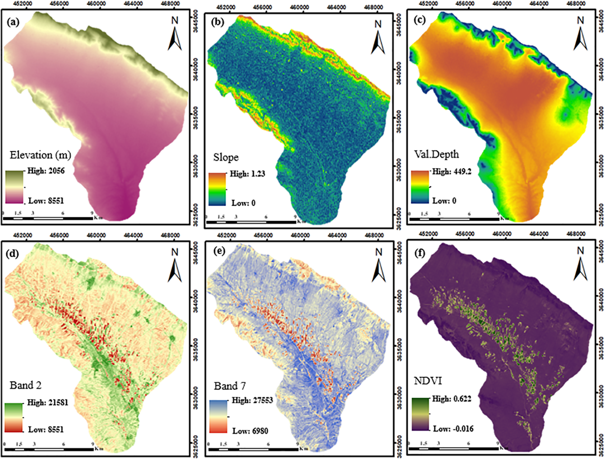
Figure 4: Six examples of auxiliary variables applied for the purpose of modeling soil organic carbon and inorganic carbon: (a) Elevation, (b) Slope, (c) Valley Depth (Val.Depth), (d) Band 2 Landsat 8 individual band, (e) Band 7, and (f) Normalized Difference Vegetation Index (NDVI)

2.4 Pre-Processing Examination

To optimize model performance, feature selection is crucial when dealing with a large pool of potential predictors. Exhaustive exploration of all possible predictor combinations is computationally impractical [23,24]. Therefore, efficient feature selection techniques are essential to identify the most influential variables. In this study, multicollinearity among variables was assessed using the Variance Inflation Factor (VIF). Variables with a VIF exceeding 10 were excluded to enhance model stability [25]. Subsequently, the Boruta algorithm was employed to select the most significant predictors for SOC and SIC [26]. To evaluate the ability of environmental variables to predict SOC and SIC from a combination of remote sensing data, topographic features, selected meteorological data, and selected land cover data, several scientific metrics were employed.

2.5 Modeling and Evaluation of Models

In order to predict SOC and SIC a nonlinear Random Forest (RF) machine learning algorithm was employed, also, all modeling processes and fitting optimization were carried out by applying the “caret” and “randomForest” (ver: 4.7-1.2) packages in R 3.5.2 [27].

Ten-fold cross-validation was applied to evaluate how well the model performed in estimating the contents of SOC and SIC [28,29]. A major strength of the ten-fold cross-validation method lies in its consistent reliability and fairness across small datasets. The four considered statistical indices were applied to evaluate the potential of predictive models for SOC and SIC, specifically, the coefficient of determination (R2), root mean square error (RMSE), mean absolute error (MAE), and normalized root mean square error (nRMSE) as shown in Eqs. (1)–(4). An appropriate predictor should have an RMSE which will be the lowest, and (R2) shows the variance proportion in the object variable that could be elucidated by the model.

R2=1−Σi=1n(Z∗(Xi)−Z(Xi))2Σi=1n(Z(Xi)−z¯(X))2(1)

RMSE=[∑i−1N[Z(Xi)−Z∗(Xi)]2N]12(2)

MAE=1NΣi=1n[|Z(Xi)−Z∗(Xi)|](3)

nRMSE=RMSEZ¯(X)(4)

where Z(Xi) and Z ∗ (Xi) show the observed and predicted values, respectively, and Z¯(X) denotes to the mean of observed values, and N signifies the measurements number.

2.6 Post-Hoc Modeling

To elucidate the RF model’s behavior in predicting SOC and SIC, variable importance analysis (via) and partial dependence plots (PDP) were employed. These techniques provided insights into the relative contributions of predictors and the nature of their relationships with the target variables [30]. Via and PDP were selected for their simplicity and effectiveness in visualizing variable effects and interactions. These methods are well-suited for soil modeling, where understanding how predictors influence outcomes both individually and in combination is important. Compared to more complex techniques like SHAP, via and PDP offer clearer insights with lower computational cost.

To assess model uncertainty, a bootstrapping approach was employed, involving repeated resampling of the dataset with replacement to estimate the variability in predictions. The overall research workflow is illustrated in Fig. 2, outlining the sequential steps of data acquisition, preprocessing, analysis, and interpretation.

3  Results and Discussion

3.1 Descriptive Statistics

A statistical summary of SOC and SIC can be seen in Table 3. The results showed that the SOC content varied from 0.19% to 1.77% with the average being 0.70%; also, the results indicated that SIC ranged from 0.36% to 6.48% with an average of 2.71.%, while the higher standard deviation for SIC showed higher variation, as compared to SOC, in the given study area. The Kolmogorov–Smirnov test confirmed the normal distribution for both variables. According to the classification applied for the coefficient of variation (CV) values, as proposed by Wilding (1985), SOC (CV = 42.85%) and SIC (CV = 45.97%) had high variability. Indeed, high CV values indicate substantial spatial variation of SOC and SIC for the whole of the given area [31]. In this study, a lower CV was obtained for SOC values, rather than SIC; this conformed to the findings achieved by [12]. The high SOC variability in the considered area may also be ascribed to different land use management and tillage practices [32,33]. Moreover, a great portion of the area is sheltered by rangelands with a high variety of vegetation cover because of different grazing pressures on the rangeland. Differences in the density of vegetation have led to the high variability of soil organic materials throughout the rangelands [34].

SIC also indicated high variation, which was presumably ascribed to variability in soil forming factors, parent material, relief, as well as tillage practices. An important factor in the SIC variability in the surface layers is related to the appearance of calcic horizons on the surface because of severe soil loss in the given area. The other main process that could control the variability of SIC in semi-arid regions is the variability of the decalcification process along the landscape [35,36]. In the studied semi-arid region, some parts including lower and stable slopes received higher moisture, and decalcification occurred to a higher extent, as compared to steep slopes. Therefore, it is expected that in these areas, lower calcium carbonates would exist in the surface layer.

3.2 Performances of Developed Models

According to the VIF method [18] and the Boruta method, the most factors were identified for explaining of the variability of SOC and SIC in the given watershed. Overall, among the chosen variables, 21 topographic attributes, seven RS indices, and four other thematic maps comprising geology, geomorphology, climatic data, and land use were included in the modeling (Table 1) for SOC and SIC in the given watershed.

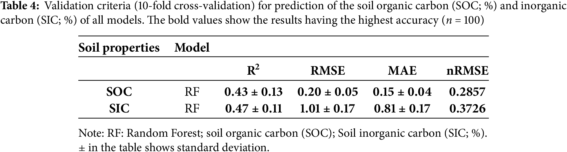
Machine learning (ML) methods have been demonstrated in numerous studies to have the potential to identify non-linear correlations among SOC, SIC, and variables [37]. Performance evaluation of the models was conducted using the R2, RMSE, nRMSE, and MAE indices (Table 4). Table 4 shows that the RF model exhibited the more accurate performance in predicting SOC with R2 (0.43 ± 0.13) and the lowest RMSE (0.20 ± 0.05), MAE (0.15 ± 0.04), and nRMSE (0.28). The moderate R2 in our study suggests that while the RF model captures key patterns, a substantial portion of the variance remains unexplained. This may be due to unmeasured variables (e.g., soil management history, microclimate effects), data noise, or inherent complexity in soil processes, that is a common limitation in spatial modeling. Similar studies modeling SOC using RF have reported R2 values ranging from 0.30 to 0.65, depending on spatial scale, input data quality, and environmental heterogeneity [38]. Our result falls within this range, particularly given the challenging semi-arid context and limited availability of high-resolution covariates. The RF model showed the best results in predicting SIC with R2 = 0.47; RMSE = 1.01 ± 0.17; MAE = 0.81 ± 0.17; nRMSE = 0.3726 (Table 4).

RF could be regarded as extensively used machine learning in DSM studies [32]. When considering other models ML, the major advantages of RF over them are its non-parametric character, its capacity to handle and employ very large variables sets with various variables kinds (categorical or continuous variables), its high performance in prediction, the random selecting of variables throughout tree construction, and its capability to handle inaccurate data [36,37]. Our results conformed to the investigations performed by [38], which shows good RF performance; meanwhile, some other scholars have reported lower accuracy for the RF model [38]. These discrepancies in the potential of different machine learning models for prediction could be related to several reasons, such as the number of soil samples and their density in the field, model multiplicity, landscape complication, type of environmental variables, source of data, and their resolution [38].

The results indicate that the inclusion of RS data in the previous auxiliary input variables (topographic attributes, precipitation, geology, geomorphology, and land use) could enhance the predictive models’ accuracy. Matinfar et al. [4], in predicting SOC in Khorramabad plain, west of Iran, showed that including RS and geomorphic attributes led to a higher performance of prediction. Moreover, Wang et al. [38] observed that superior results were achieved when the derived topographic variables, as well as RS, were applied together for prediction. The findings demonstrated that both models performed better than individual variable sets in estimating SOC and SIC [39]. Accordingly, some scholars [39] employed Sentinel-1, Sentinel-2, and topographic parameters as the auxiliary environmental variables for predicting SOC and total nitrogen. They reported that the scenario with all three data sets had a higher performance than other variable arrays for estimating SOC and total nitrogen. Our findings also indicated that the variable set with higher comprehensiveness had a higher performance than the limited variables [40].

3.3 Relative Importance and PDP Analysis

3.3.1 Variable Importance

To attain a thorough thoughtful of the environmental variables that were more imperative in the prediction of the SOC content, the via based on the RF model is presented in Fig. 5. According to the via, the land cover map was identified to be the most significant variable for the SOC prediction. A study conducted in Iran [41] showed that diverse land-uses led to significant changes in the SOC contents. Other scholars [42,43] had the prediction of a higher SOC content in agricultural lands, as compared to other land uses in western Iran and North-Western France, respectively. On the contrary, another research [44] indicated that the change of land uses had a minimal impact on the content of SOC.

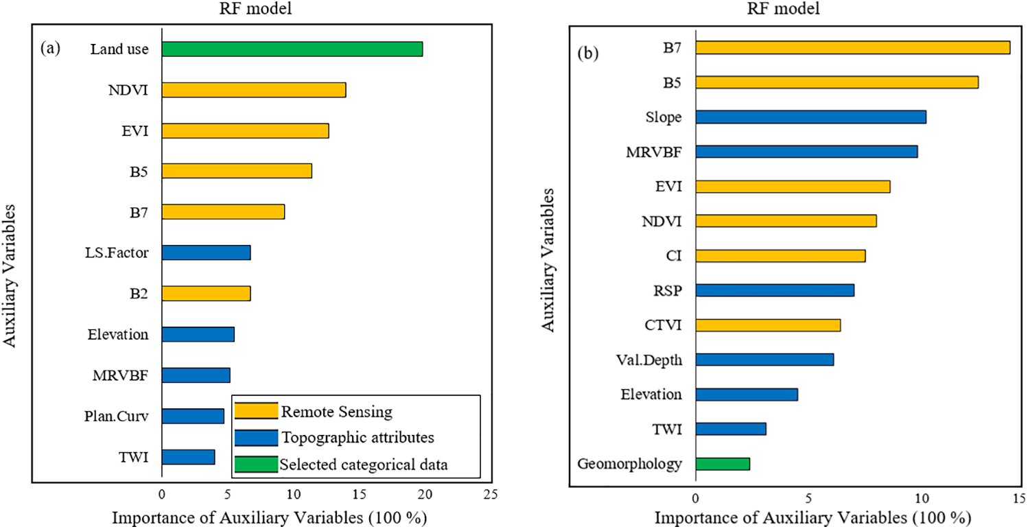
Figure 5: The relative importance of each of environmental variables (%) for the prediction of soil organic carbon and soil inorganic carbon in various datasets according to RF model. Soil organic carbon (a); soil inorganic carbon (b). NDVI: Normalized vegetation index, EVI: Enhanced vegetation index, B1, …, B7 are the bands of Landsat, MRVBF: Multi-resolution Valley Bottom Flatness, CI: Carbonate index; CTVI: Corrected Transformed Ratio Vegetation Index, TWI: Topographic wetness index; LS: slope-length factor; Plan. Curv: Plan Curvature

Following the land use map, RS indices were identified as the most significant variables for estimating SOC. The ranking and their contributions in estimating SOC were as follows: NDVI > EVI > B5 > B7 > B2. RS indices are commonly regarded as worthy estimators of SOC content, as Wang et al. [44]. SOC can influence the shape and intensity of the soil’s reflectance spectrum. In general, soils having more organic matter appear to be darker. In addition, concerning diverse compositions of SOM, reflectance occurs in the mid to thermal infrared range (2500–25,000 nm), as well as in the visible range (400–700 nm) [45]. Therefore, the existence of relationships between soil features and the reflectance spectrum in the specific wavelengths could lead to the cost-effective estimation of SOC [46]. Hence, the high contributions of NDVI, as the most well-known indicator of soil organic matter existence and other bands (B2, B5, and B7) (Fig. 5), obviously corresponded to the reflectance behavior of soil organic matter in the wide electromagnetic spectrum range [47]. Band 5 (Near Infrared, ~0.85–0.88 μm) is sensitive to vegetation and organic matter due to its interaction with molecular vibrations and water content in soils. Organic matter tends to absorb energy in this range, contributing to darker soil reflectance. This band is particularly useful for detecting SOC through vegetation indices such as NDVI and EVI, which are derived from NIR reflectance. Band 7 (Shortwave Infrared 2, ~2.11–2.29 μm) is highly responsive to carbonate minerals due to strong absorption features associated with CO32− molecular vibrations. Carbonates exhibit distinct reflectance peaks in this region, making Band 7 a reliable indicator for SIC detection. Asgari et al. [48] demonstrated that carbonate content significantly increases reflectance intensity in SWIR bands, especially around 2338 nm.

Following the RS indices, some topographic attributes including the LS factor, elevation, MRVBF, plan curvature, and topographic wetness index (TWI) were deemed as the most imperative topographic attributes to account for the SOC variability in the area. All these terrain attributes, directly or indirectly, can control the redistribution of soil particles (especially SOC), energy, and water through the watershed [49]. Dai et al. [50] had the observation of strong relationships between the SOC content and NDVI, precipitation, elevation, and temperature. Several studies have previously revealed that topographic attributes, via effects on soil erosion as well as deposition processes, could be important in determining SOC stability and accumulation [2,32]. A strong association between the SOC content and slope was reported by Fissore et al. [51], stating that topographic attributes could do the regulation of SOC dynamics as well as SOC quality.

Based on the findings of via for SIC, by RF model, RS data, and topographic attributes were acknowledged as the most significant variables. Band 7 (Short wave Infrared 2, SWIR2) in the range of 2.11–2.29 μm and Band 5 (Near infrared, NIR) in the range of 0.85–0.88 μm were the most persuasive variables in the 1st and 2nd ranking. Asgari et al. [48], in studying carbonatic soils, reported the specific absorption wavelength as the soil carbonates incidence was 2.338 μ, which was intensified with the carbonates content; this was in synchrony with Band 7 of ETM+ data. Such observations conformed to the findings obtained by [52,53]. Interestingly, the carbonate index (CI) was identified as one of the top ten influential variables for predicting SIC in this study (Fig. 5).

Among the topographic attributes, slope, MRVBF, relative slope position (RSP), valley depth, elevation, and TWI were recognized as the topographic attributes that had considerable impacts on the distribution of carbonates in the given area (see Fig. 5). Topographic attributes could significantly mediate the carbonate distribution throughout the landscape because of the effects of topography on soil formation processes and soil erosion. In steep slopes, severe sheet erosion leads to the appearance of subsurface horizons that are enriched by calcium carbonates [54]. The Wetness Index as the proxy of water and moisture patterns along the landscape serves a vital role in the distribution of carbonates as relatively soluble minerals [55]. Soil-forming processes along different slope positions also mediate the distribution of carbonates in semi-arid regions. Calcium carbonates are likely to transfer from higher to lower slope positions; they can accumulate on some specific land surfaces as a consequence of slope hydrology. Therefore, several topographic attributes like slope, curvature, catchment area, and upslope area, by inducing the hydrological circumstances of a location and making diverse soil moisture conditions, may generate different patterns of carbonate leaching [55]. According to the results of via, geomorphology was recognized as the influential variable that could control the variability of SIC. The highest values of SIC were observed in alluvial plains in the given area. Sreenivas et al. [3], in a study, stated that alluvial plains had variable SIC content because of the variation in the alluviums set down throughout the watershed.

Among the selected variables, unexpectedly, climatic variables were not included as the most significant variables for modeling SOC and SIC. Although several studies have proved that climatic variables have a great involvement in the SOC and SIC variability [32], it seems that the low importance of these variables relates to the very low variation of climatic conditions in the studied catchment.

3.3.2 Partial Dependence Plot Analysis

To understand how the most important factors influence the outcome, we conducted a PDP analysis on the top four predictors identified by our most accurate ML model (Fig. 6). A PDP plot illustrates how SOC contents change in response to varying levels of environmental factors. The x-axis represents the values or categories of each factor, while the y-axis shows the average SOC or SIC value corresponding to those levels. According to the analysis, land use, NDVI, EVI, and B5 were the most influential factors in predicting SOC. (Fig. 5a). In the left and right panels, higher amounts of SOC are associated with high values of EVI, NDVI, and Land use where vegetation cover is dense and the wetness shows a rather monotonous positive effect. Three plots are supported by the response curves (Fig. 6a–c). The response curve of SOC to EVI and NDVI variation showed that SOC increased with increasing vegetation cover. Also, the land-cover plot that agricultural land use has the highest amount of SOC. In similar studies, Peng et al. [56] reported the very important effect of vegetation-related indices such as EVI and NDVI on the SOC variation, as well as, for SIC prediction, the most important variables were B7, B5, Slope, and MRVBF (Fig. 5b). The results of the PDP for these four key variables are shown in Fig. 7, where the results showed that SIC content increases with MRVBF, while it decreases with Slope. Generally, the steeper the slope, the greater the erosion, and the less soil formation and vegetation cover is expected [57].

Figure 6: Response of SOC accumulation (%) to the variation of each predictive factor. (a) Land use, (b) Normalized Difference Vegetation Index (NDVI), (c) Enhanced Vegetation Index (EVI), (d) Band 5

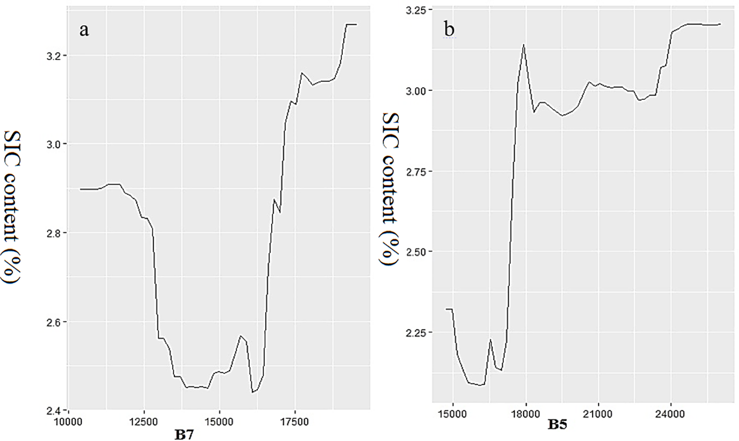
Figure 7: Response of SIC accumulation (%) to the variation of each predictive factor. (a) Band 7, (b) Band 5, (c) Slope, (d) Multi-resolution Valley Bottom Flatness Index (MRVBF)

3.4 Spatial Prediction of SOC and SIC and Uncertainty Mapping

The spatial prediction maps of SOC and SIC are presented in Fig. 8. Fig. 8a represents the SOC map derived using terrain attributes, climatic data, categorical data, and RS data by the RF model. The values of SOC varied from 0.22% to 1.34%.

Figure 8: Spatial prediction and uncertainty map of SOC and SIC (%) applying the RF model. (a) Spatial prediction SOC, (b) uncertainty map SOC, (c) Spatial prediction SIC, (d) uncertainty map SIC

The maximum values of SOC were observed in the central parts of the watershed, which were mostly covered by irrigated farming. As can be seen in the land use map (Fig. 3a), there were some irrigated crops (wheat, barley, alfalfa, …) in the central parts of the watershed with a low slope gradient. Returning crop residues and the application of manure by local farmers [58] have led to an increase in SOC in these portions of the watershed. Similarly, Mousavi et al. [29] predicted higher mean SOC in agricultural lands, as compared to other land uses, across the landscape. Meanwhile, in the steep slopes with overgrazed areas and high intensity of soil erosion, the minimum SOC was observed (Fig. 5a). Several researchers have reported similar results, showing that overgrazing on steep slopes led to severe sheet erosion and eventually, soil organic material loss [53].

Spatial scattering of SIC, resulting from RF models is shown in Fig. 8c. The spatial distribution of SIC derived from the RF model on the selected variables is illustrated in Fig. 8c. The results extracted from topographic features, climatic data, classified data (geology, geomorphology, and land use), and remote sensing data by the RF model in this map ranged from 0.38 to 5.05 percent. The uncertainty map also showed almost very low uncertainty involved with the predicted SIC map with a standard deviation between 0.03 and 0.70. According to Fig. 8d (right panel), the highest uncertainty associated with SIC prediction was seen in the center parts of the study area.

The SIC uppermost values were perceived in the north and central parts of the studied watershed. In the northern parts, along with the presence of calcareous rock-outs, calcium carbonates were exposed to the surface and the highest contents were recorded. In the central parts of the studied watershed with the lowest elevation, the higher SIC was related to receiving carbonates from the highlands as a consequence of soil erosion. Several scholars in arid and semi-arid regions have reported that soluble compounds such as calcite are transported and redistributed in the lowlands following soil erosion and deposition processes [59].

The uncertainty map for the predicted SOC and SIC is presented in Fig. 8b,d, right panels. In general, very low uncertainty is associated with the predicted map, showing the reliability of the implemented model and results (SOC: PI = 0.005%–0.27%, SIC: PI = 0.03%–0.70%). Nevertheless, almost all of the highest amounts of uncertainty are seen in areas with the lowest SOC content, and vs. for SIC the highest uncertainty was observed in the central part of the study area. Zhao et al. [60] posited that the bootstrap method is effective in quantifying uncertainty within RF models. They emphasized that by addressing various factors—such as minimizing measurement errors, capturing spatial correlations, and selecting appropriate scales—researchers can improve the reliability and informative quality of prediction maps. This approach aligns with the principles of SOC and SIC, where reducing uncertainty enhances the understanding of soil dynamics and contributes to more accurate predictions in environmental modeling.

4  Conclusions

The present study examined the spatial variability of SOC and SIC in a semi-arid watershed in central Iran using the RF model and a diverse set of environmental variables. The results revealed that land use was the most influential factor in SOC prediction, followed by remote sensing indices such as NDVI and EVI, and then topographic attributes. The high SOC content observed in irrigated farmlands is likely due to crop residue inputs, which explains the strong correlation between SOC distribution and land use. For SIC modeling, RS data proved to be the most effective predictors, primarily due to the distinct spectral signatures of carbonates. Geomorphological features and topographic attributes also played a critical role, reflecting the impact of hydrological and hydropedological processes on SIC distribution. Partial dependence plots (PDPs) effectively illustrated non-linear relationships between environmental variables and SOC/SIC predictions, enhancing the interpretability and transparency of the RF model. Climatic variables, however, showed limited contribution to SOC and SIC prediction, likely due to low climatic variability across the study area. This suggests the need for further evaluation of climate-related variables in larger or more diverse semi-arid catchments. Overall, the findings have important implications for land management and carbon sequestration strategies in semi-arid regions. Identifying key environmental drivers such as land use, vegetation indices, and terrain attributes enables more targeted interventions to enhance soil carbon stocks. Future research should focus on testing model generalizability across broader geographic settings, incorporating higher-resolution data, and exploring alternative machine learning algorithms to further refine predictive accuracy and support sustainable land-use planning.

Acknowledgement: The authors gratefully acknowledge the financial support provided by the University of Isfahan, which made this research possible.

Funding Statement: The Iranian National Science Foundation (INSF) provided financial support for this research under Project Number 4004169, and the authors would like to thank Isfahan University of Technology and the University of Isfahan for their valuable contributions.

Author Contributions: Shohreh Moradpour: Filed study, laboratory analysis and formal analysis; Shuai Zhao: Support, supervision and revision the manuscript; Mojgan Entezari: Supervision; Shamsollah Ayoubi: Conceptualization and revising the final version; Seyed Roohollah Mousavi: Data analysis and modeling. All authors reviewed the results and approved the final version of the manuscript.

Availability of Data and Materials: Data are available by the request on authors.

Ethics Approval: Not applicable.

Conflicts of Interest: The authors declare no conflicts of interest to report regarding the present study.

References

1. Ma HP, Yang XL, Guo QQ, Zhang XJ, Zhou CN. Soil organic carbon pool along different altitudinal level in the Sygera Mountains, Tibetan Plateau. J Mt Sci. 2016;13(3):476–83. doi:10.1007/s11629-014-3421-6. [Google Scholar] [CrossRef]

2. Chi Y, Liu D, Xie Z. Zonal simulations for soil organic carbon mapping in coastal wetlands. Ecol Indic. 2021;132:108291. doi:10.1016/j.ecolind.2021.108291. [Google Scholar] [CrossRef]

3. Sreenivas K, Dadhwal VK, Kumar S, Harsha GS, Mitran T, Sujatha G, et al. Digital mapping of soil organic and inorganic carbon status in India. Geoderma. 2016;269:160–73. doi:10.1016/j.geoderma.2016.02.002. [Google Scholar] [CrossRef]

4. Matinfar HR, Maghsodi Z, Mousavi SR, Rahmani A. Evaluation and prediction of topsoil organic carbon using machine learning and hybrid models at a field-scale. Catena. 2021;202:105258. doi:10.1016/j.catena.2021.105258. [Google Scholar] [CrossRef]

5. Goydaragh MG, Taghizadeh-Mehrjardi R, Jafarzadeh AA, Triantafilis J, Lado M. Using environmental variables and fourier transform infrared spectroscopy to predict soil organic carbon. Catena. 2021;202:105280. doi:10.1016/j.catena.2021.105280. [Google Scholar] [CrossRef]

6. Shafizadeh-Moghadam H, Minaei F, Talebi-khiavi H, Xu T, Homaee M. Synergetic use of multi-temporal Sentinel-1, Sentinel-2, NDVI, and topographic factors for estimating soil organic carbon. Catena. 2022;212:106077. doi:10.1016/j.catena.2022.106077. [Google Scholar] [CrossRef]

7. Batjes NH. Total carbon and nitrogen in the soils of the world. Eur J Soil Sci. 1996;47(2):151–63. doi:10.1111/j.1365-2389.1996.tb01386.x. [Google Scholar] [CrossRef]

8. Marchant BP, Villanneau EJ, Arrouays D, Saby NPA, Rawlins BG. Quantifying and mapping topsoil inorganic carbon concentrations and stocks: approaches tested in France. Soil Use Manage. 2015;31(1):29–38. doi:10.1111/sum.12158. [Google Scholar] [CrossRef]

9. Grinand C, Barthès BG, Brunet D, Kouakoua E, Arrouays D, Jolivet C, et al. Prediction of soil organic and inorganic carbon contents at a national scale (France) using mid-infrared reflectance spectroscopy (MIRS). Eur J Soil Sci. 2012;63(2):141–51. doi:10.1111/j.1365-2389.2012.01429.x. [Google Scholar] [CrossRef]

10. Liu X, Lu X, Yu R, Sun H, Li X, Li X, et al. Distribution and storage of soil organic and inorganic carbon in steppe riparian wetlands under human activity pressure. Ecol Indic. 2022;139:108945. doi:10.1016/j.ecolind.2022.108945. [Google Scholar] [CrossRef]

11. Boubehziz S, Khanchoul K, Benslama M, Benslama A, Marchetti A, Francaviglia R, et al. Predictive mapping of soil organic carbon in Northeast Algeria. Catena. 2020;190:104539. doi:10.1016/j.catena.2020.104539. [Google Scholar] [CrossRef]

12. Zeraatpisheh M, Ayoubi S, Jafari A, Tajik S, Finke P. Digital mapping of soil properties using multiple machine learning in a semi-arid region, central Iran. Geoderma. 2019;338:445–52. doi:10.1016/j.geoderma.2018.09.006. [Google Scholar] [CrossRef]

13. Fathololoumi S, Vaezi AR, Alavipanah SK, Ghorbani A, Saurette D, Biswas A. Improved digital soil mapping with multitemporal remotely sensed satellite data fusion: a case study in Iran. Sci Total Environ. 2020;721:137703. doi:10.1016/j.scitotenv.2020.137703. [Google Scholar] [PubMed] [CrossRef]

14. Zhou T, Geng Y, Chen J, Pan J, Haase D, Lausch A. High-resolution digital mapping of soil organic carbon and soil total nitrogen using DEM derivatives, Sentinel-1 and Sentinel-2 data based on machine learning algorithms. Sci Total Environ. 2020;729:138244. doi:10.1016/j.scitotenv.2020.138244. [Google Scholar] [PubMed] [CrossRef]

15. Naimi S, Ayoubi S, Demattê JAM, Zeraatpisheh M, Amorim MTA, de Oliveira Mello FA. Spatial prediction of soil surface properties in an arid region using synthetic soil image and machine learning. Geocarto Int. 2022;37(25):8230–53. doi:10.1080/10106049.2021.1996639. [Google Scholar] [CrossRef]

16. Mohammadi S, Habashi K, Pourmanafi S. Monitoring and forecasting land use/cover changes and its relationship with drought (study Zayandeh Rood watershedcase B: sub-parcel basin. Remote Sens Geogr Inf Syst Nat Resour. 2018;9(1):24–39. [Google Scholar]

17. Liaghati H, Rahnama F. Sediment measurement and erosion process investigation by regional and direct method and using remote sensing in one of the watershed sub-basins of Parcel B2 of Zayandeh Rood Dam, Isfahan. In: National Conference of Watershed Sciences and Engineering of Iran; 2006 Feb 14–15; Tehran, Iran. [Google Scholar]

18. Lai YQ, Wang HL, Sun XL. A comparison of importance of modelling method and sample size for mapping soil organic matter in Guangdong. China Ecol Indic. 2021;126:107618. doi:10.1016/j.ecolind.2021.107618. [Google Scholar] [CrossRef]

19. Black CA. Method of soil analysis, part 2, chemical and microbiological properties. Madison, WI, USA: American Society of Agronomy, Inc.; 1965. [Google Scholar]

20. Gholizadeh A, Žižala D, Saberioon M, Borůvka L. Soil organic carbon and texture retrieving and mapping using proximal, airborne and Sentinel-2 spectral imaging. Remote Sens Environ. 2018;218:89–103. doi:10.1016/j.rse.2018.09.015. [Google Scholar] [CrossRef]

21. Bakhshandeh E, Zeraatpisheh M, Soleimani A, Francaviglia R. Land use conversion, climate change and soil organic carbon: modeling a citrus garden chronosequence in Northern Iran. Geoderma Reg. 2022;30:e00559. doi:10.1016/j.geodrs.2022.e00559. [Google Scholar] [CrossRef]

22. Jafari A, Ayoubi S, Khademi H, Finke PA, Toomanian N. Selection of a taxonomic level for soil mapping using diversity and map purity indices: a case study from an Iranian arid region. Geomorphology. 2013;201:86–97. doi:10.1016/j.geomorph.2013.06.010. [Google Scholar] [CrossRef]

23. Scull P, Franklin J, Chadwick OA. The application of classification tree analysis to soil type prediction in a desert landscape. Ecol Model. 2005;181(1):1–15. doi:10.1016/j.ecolmodel.2004.06.036. [Google Scholar] [CrossRef]

24. Ließ M, Schmidt J, Glaser B. Improving the spatial prediction of soil organic carbon stocks in a complex tropical mountain landscape by methodological specifications in machine learning approaches. PLoS One. 2016;11(4):e0153673. doi:10.1371/journal.pone.0153673. [Google Scholar] [PubMed] [CrossRef]

25. Mousavi SR, Sarmadian F, Omid M, Bogaert P. Three-dimensional mapping of soil organic carbon using soil and environmental covariates in an arid and semi-arid region of Iran. Measurement. 2022;201:111706. doi:10.1016/j.measurement.2022.111706. [Google Scholar] [CrossRef]

26. Rezaei M, Mousavi SR, Rahmani A, Zeraatpisheh M, Rahmati M, Pakparvar M, et al. Incorporating machine learning models and remote sensing to assess the spatial distribution of saturated hydraulic conductivity in a light-textured soil. Comput Electron Agric. 2023;209:107821. doi:10.1016/j.compag.2023.107821. [Google Scholar] [CrossRef]

27. Team RC. R: a language and environment for statistical computing. Vienna, Austria: R Foundation for Statistical Computing; 2019. [Google Scholar]

28. Naimi S, Ayoubi S, Zeraatpisheh M, Dematte JAM. Ground observations and environmental covariates integration for mapping of soil salinity: a machine learning-based approach. Remote Sens. 2021;13(23):4825. doi:10.3390/rs13234825. [Google Scholar] [CrossRef]

29. Mousavi SR, Jahandideh Mahjenabadi VA, Khoshru B, Rezaei M. Spatial prediction of winter wheat yield gap: agro-climatic model and machine learning approaches. Front Plant Sci. 2023;14:1309171. doi:10.3389/fpls.2023.1309171. [Google Scholar] [PubMed] [CrossRef]

30. Su L, Heydari M, Jaafarzadeh MS, Mousavi SR, Rezaei M, Fathizad H, et al. Incorporating forest canopy openness and environmental covariates in predicting soil organic carbon in oak forest. Soil Tillage Res. 2024;244:106220. doi:10.1016/j.still.2024.106220. [Google Scholar] [CrossRef]

31. Mahmoudzadeh H, Matinfar HR, Taghizadeh-Mehrjardi R, Kerry R. Spatial prediction of soil organic carbon using machine learning techniques in western Iran. Geoderma Reg. 2020;21:e00260. doi:10.1016/j.geodrs.2020.e00260. [Google Scholar] [CrossRef]

32. Ajami M, Heidari A, Khormali F, Gorji M, Ayoubi S. Environmental factors controlling soil organic carbon storage in loess soils of a subhumid region, northern Iran. Geoderma. 2016;281:1–10. doi:10.1016/j.geoderma.2016.06.017. [Google Scholar] [CrossRef]

33. Rostaminia M, Rahmani A, Mousavi SR, Taghizadeh-Mehrjardi R, Maghsodi Z. Spatial prediction of soil organic carbon stocks in an arid rangeland using machine learning algorithms. Environ Monit Assess. 2021;193(12):815. doi:10.1007/s10661-021-09543-8. [Google Scholar] [PubMed] [CrossRef]

34. Chenchouni H, Neffar S. Soil organic carbon stock in arid and semi-arid steppe rangelands of North Africa. Catena. 2022;211:106004. doi:10.1016/j.catena.2021.106004. [Google Scholar] [CrossRef]

35. Garosi Y, Sheklabadi M, Conoscenti C, Pourghasemi HR, Van Oost K. Assessing the performance of GIS-based machine learning models with different accuracy measures for determining susceptibility to gully erosion. Sci Total Environ. 2019;664:1117–32. doi:10.1016/j.scitotenv.2019.02.093. [Google Scholar] [PubMed] [CrossRef]

36. Herrmann N, Stadtmann R, Meister J, Kirchner A. Importance of substrate genesis for Mediterranean soil evolution—an example from a limestone hillslope in the Estremadura (W-Portugal). Catena. 2022;218:106566. doi:10.1016/j.catena.2022.106566. [Google Scholar] [CrossRef]

37. Wang S, Adhikari K, Zhuang Q, Yang Z, Jin X, Wang Q, et al. An improved similarity-based approach to predicting and mapping soil organic carbon and soil total nitrogen in a coastal region of northeastern China. PeerJ. 2020;8:e9126. doi:10.7717/peerj.9126. [Google Scholar] [PubMed] [CrossRef]

38. Wang S, Gao J, Zhuang Q, Lu Y, Gu H, Jin X. Multispectral remote sensing data are effective and robust in mapping regional forest soil organic carbon stocks in a northeast forest region in China. Remote Sens. 2020;12(3):393. doi:10.3390/rs12030393. [Google Scholar] [CrossRef]

39. Zhou T, Geng Y, Ji C, Xu X, Wang H, Pan J, et al. Prediction of soil organic carbon and the C:N ratio on a national scale using machine learning and satellite data: a comparison between Sentinel-2, Sentinel-3 and Landsat-8 images. Sci Total Environ. 2021;755(Pt 2):142661. doi:10.1016/j.scitotenv.2020.142661. [Google Scholar] [PubMed] [CrossRef]

40. Wang J, Peng J, Li H, Yin C, Liu W, Wang T, et al. Soil salinity mapping using machine learning algorithms with the sentinel-2 MSI in arid areas, China. Remote Sens. 2021;13(2):305. doi:10.3390/rs13020305. [Google Scholar] [CrossRef]

41. Taghizadeh-Mehrjardi R, Nabiollahi K, Kerry R. Digital mapping of soil organic carbon at multiple depths using different data mining techniques in Baneh region. Iran Geoderma. 2016;266:98–110. doi:10.1016/j.geoderma.2015.12.003. [Google Scholar] [CrossRef]

42. Lacoste M, Minasny B, McBratney A, Michot D, Viaud V, Walter C. High resolution 3D mapping of soil organic carbon in a heterogeneous agricultural landscape. Geoderma. 2014;213:296–311. doi:10.1016/j.geoderma.2013.07.002. [Google Scholar] [CrossRef]

43. Bierer AM, Leytem AB, Dungan RS, Moore AD, Bjorneberg DL. Soil organic carbon dynamics in semi-arid irrigated cropping systems. Agronomy. 2021;11(3):484. doi:10.3390/agronomy11030484. [Google Scholar] [CrossRef]

44. Wang B, Waters C, Orgill S, Gray J, Cowie A, Clark A, et al. High resolution mapping of soil organic carbon stocks using remote sensing variables in the semi-arid rangelands of eastern Australia. Sci Total Environ. 2018;630:367–78. doi:10.1016/j.scitotenv.2018.02.204. [Google Scholar] [PubMed] [CrossRef]

45. Shepherd KD, Walsh MG. Development of reflectance spectral libraries for characterization of soil properties. Soil Sci Soc Am J. 2002;66(3):988. doi:10.2136/sssaj2002.0988. [Google Scholar] [CrossRef]

46. Ladoni M, Ali Bahrami H, Alavipanah SK, Norouzi AA. Estimating soil organic carbon from soil reflectance: a review. Precis Agric. 2010;11(1):82–99. doi:10.1007/s11119-009-9123-3. [Google Scholar] [CrossRef]

47. Brown DJ, Shepherd KD, Walsh MG, Dewayne Mays M, Reinsch TG. Global soil characterization with VNIR diffuse reflectance spectroscopy. Geoderma. 2006;132(3–4):273–90. doi:10.1016/j.geoderma.2005.04.025. [Google Scholar] [CrossRef]

48. Asgari N, Ayoubi S, Demattê JAM, Dotto AC. Carbonates and organic matter in soils characterized by reflected energy from 350–25,000 nm wavelength. J Mt Sci. 2020;17(7):1636–51. doi:10.1007/s11629-019-5789-9. [Google Scholar] [CrossRef]

49. Kwang JS, Thaler EA, Quirk BJ, Quarrier CL, Larsen IJ. A landscape evolution modeling approach for predicting three-dimensional soil organic carbon redistribution in agricultural landscapes. J Geophys Res Biogeosci. 2022;127(2):e2021JG006616. doi:10.1029/2021JG006616. [Google Scholar] [CrossRef]

50. Dai F, Zhou Q, Lv Z, Wang X, Liu G. Spatial prediction of soil organic matter content integrating artificial neural network and ordinary Kriging in Tibetan Plateau. Ecol Indic. 2014;45:184–94. doi:10.1016/j.ecolind.2014.04.003. [Google Scholar] [CrossRef]

51. Fissore C, Dalzell BJ, Berhe AA, Voegtle M, Evans M, Wu A. Influence of topography on soil organic carbon dynamics in a Southern California grassland. Catena. 2017;149:140–9. doi:10.1016/j.catena.2016.09.016. [Google Scholar] [CrossRef]

52. Viscarra Rossel RA, Cattle SR, Ortega A, Fouad Y. In situ measurements of soil colour, mineral composition and clay content by vis-NIR spectroscopy. Geoderma. 2009;150(3–4):253–66. doi:10.1016/j.geoderma.2009.01.025. [Google Scholar] [CrossRef]

53. Wang G, Mao J, Fan L, Ma X, Li Y. Effects of climate and grazing on the soil organic carbon dynamics of the grasslands in Northern Xinjiang during the past twenty years. Glob Ecol Conserv. 2022;34:e02039. doi:10.1016/j.gecco.2022.e02039. [Google Scholar] [CrossRef]

54. Khayamim F, Wetterlind J, Khademi H, Jean Robertson AH, Cano AF, Stenberg B. Using visible and near infrared spectroscopy to estimate carbonates and gypsum in soils in arid and subhumid regions of Isfahan. Iran J Infrared Spectrosc. 2015;23(3):155–65. doi:10.1255/jnirs.1157. [Google Scholar] [CrossRef]

55. Alijani Z, Sarmadian F. The role of topography in changing of soil carbonate content. Indian J Sci Res. 2014;6(1):263–71. [Google Scholar]

56. Peng Y, Xiong X, Adhikari K, Knadel M, Grunwald S, Greve MH. Modeling soil organic carbon at regional scale by combining multi-spectral images with laboratory spectra. PLoS One. 2015;10(11):e0142295. doi:10.1371/journal.pone.0142295. [Google Scholar] [PubMed] [CrossRef]

57. Liu D, Wang Z, Zhang B, Song K, Li X, Li J, et al. Spatial distribution of soil organic carbon and analysis of related factors in croplands of the black soil region, Northeast China. Agric Ecosyst Environ. 2006;113(1–4):73–81. doi:10.1016/j.agee.2005.09.006. [Google Scholar] [CrossRef]

58. Powlson DS, Poulton PR, Glendining MJ, MacDonald AJ, Goulding KWT. Is it possible to attain the same soil organic matter content in arable agricultural soils as under natural vegetation? Outlook Agric. 2022;51(1):91–104. doi:10.1177/00307270221082113. [Google Scholar] [CrossRef]

59. Pawlik Ł, Okupny D, Kroh P, Cybul P, Stachowicz-Rybka R, Sady-Bugajska A. Changing natural conditions and their impact on the Mt. Śnieżnica landscape, outer Western Carpathians—reconstruction of the Holocene environment based on geochemical indices and radiocarbon dating. Sci Total Environ. 2022;850:158066. doi:10.1016/j.scitotenv.2022.158066. [Google Scholar] [PubMed] [CrossRef]

60. Zhao S, Ayoubi S, Mousavi SR, Ahmad Mireei S, Shahpouri F, Wu SX, et al. Integrating proximal soil sensing data and environmental variables to enhance the prediction accuracy for soil salinity and sodicity in a region of Xinjiang Province, China. J Environ Manage. 2024;364:121311. doi:10.1016/j.jenvman.2024.121311. [Google Scholar] [PubMed] [CrossRef]