Atmospheric Delay Correction Using GNSS and GACOS Data in InSAR Land Subsidence Monitoring over Banting, Selangor

1  Introduction

Land subsidence is a global phenomenon defined as a gradual settling or sudden sinking of the earth’s surface due to the removal or displacement of subsurface earth materials [1]. Land subsidence has become a global problem due to several factors, including groundwater extraction, construction of high-rise buildings, sinkhole formation, underground mine collapse, rapid land development and natural hazards [2]. A study of 290 subsidence cases by Bagheri-Gavkosh et al. (2021) found that human-induced subsidence accounted for 76.92% of global cases [3]. Thus, there is an increasing demand for monitoring the spatial and temporal distribution of land subsidence.

Interferometric Synthetic Aperture Radar (InSAR) is a remote sensing technique that uses radar satellite images to measure ground surface deformation with millimetre-level accuracy. InSAR leverages the phase differences between two or more Synthetic Aperture Radar (SAR) images acquired at different times to generate interferograms, which reveal changes in elevation caused by land subsidence, earthquakes, or volcanic activity [4].

A major challenge in InSAR measurements is atmospheric delay, particularly due to water vapor in the troposphere, the lowest region of the atmosphere extending from the earth’s surface to approximately 10 km height. Tropospheric water vapor delay is among the most significant sources of error in InSAR measurements. Since radar signals travel through the atmosphere, variations in humidity and temperature can alter the signal phase, leading to errors in land subsidence estimates.

Previous studies on GNSS and GACOS integration have largely focused on mid-latitude regions. Limited research has evaluated their performance for atmospheric delay correction in tropical regions such as Malaysia, where water vapor distribution is more complex. This study analyzes the effectiveness of GNSS and GACOS integration under these challenging tropical conditions. Furthermore, according to Hashim et al. [5], research on atmospheric delay correction in Malaysia remains limited, as most existing studies have predominantly concentrated on landslides and floods as the country’s major natural hazards. The study area, Banting, located near the sea, experiences high water vapor concentrations due to increased sea evaporation (Smith et al., 2020), making it an ideal site for evaluating atmospheric correction methods.

Several methods exist to mitigate water vapour delay, including linear detrending, weather models and GNSS-derived corrections [6]. The use of GNSS for measuring and assessing atmospheric corrections has several benefits, such as improved spatial-temporal resolution, cost effectiveness, worldwide coverage, weather independent or unaffected by rain or clouds and excellent accuracy and [7]. GNSS measurements are particularly suitable for determining the atmospheric correction or Zenith Tropospheric Delay (ZTD) values without additional equipment, as a large portion of the GNSS Continuously Operating Reference Stations (CORS) network architecture is already operational.

The Generic Atmospheric Correction Online Service (GACOS) provides ZTD derived from numerical weather models, offering a gridded representation of tropospheric delay maps with extensive spatial coverage, though potentially subject to model-related biases [8]. This study proposes an innovative approach that integrates GNSS and GACOS data to improve atmospheric correction for land subsidence monitoring. GNSS data allows for precise measurements of ground movement, while GACOS data provides information on atmospheric conditions that affect measurement accuracy. Combining these data sources enhances land subsidence monitoring and improves understanding of contributing factors.

2  Data and Method

2.1 Study Area

The study area was located in Banting, a town in the Kuala Langat District of Selangor, Malaysia, as shown in Fig. 1. Banting is a town in the Kuala Langat District of Selangor, Malaysia. It is situated on the banks of the Langat River and near the shore of Malacca.

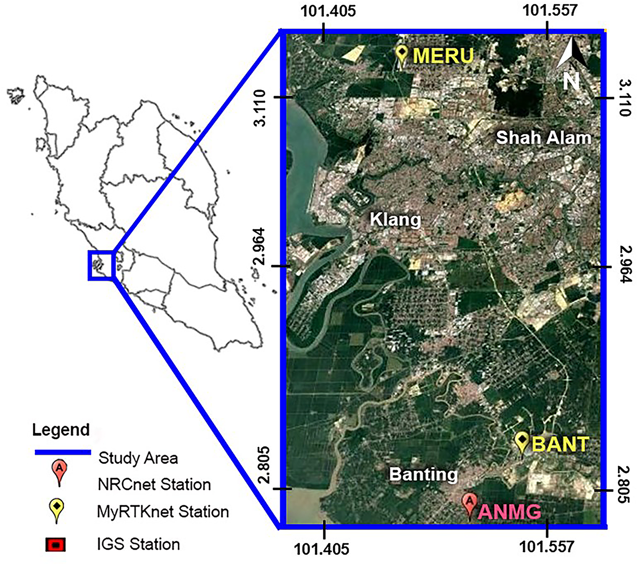
Figure 1: Study area of Banting, Selangor

Banting was chosen due to its geological and environmental characteristics. According to the Department of Mineral and Geosciences (JMG), approximately 80% of the area consists of Quaternary deposits, including marine and continental sediments such as clay, silt, sand, and peat. Notably, marine clay exhibits high susceptibility to land subsidence due to its high compressibility and tendency to consolidate under stress [9]. The area has also experienced land subsidence events. On 20 July 2020, soil erosion and sedimentation occurred near Jalan Klang-Banting due to the boring of piles for the construction of the Light Rail Transit 3 (LRT3) pile construction [10]. The road was completely closed, and the affected area was cordoned off. Furthermore, an excavator driver was killed after being crushed in a landslide at a mine in Jalan Sungai Kelambu, Banting [11]. The mine is faced heavy rain before the incident happened. Therefore, the soil type and the reported land subsidence incident in Banting make the area interesting for the study.

2.2 Data Collection

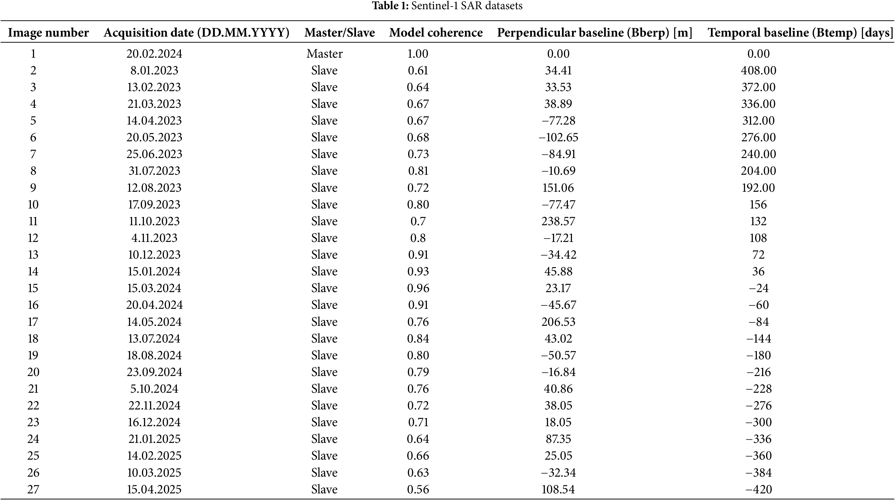
A total of 27 Sentinel-1 images from January 2023 to April 2025 were downloaded from the Sentinel Copernicus Browser (https://browser.dataspace.copernicus.eu/, accessed on 01 July 2025) [12]. Images were acquired in vertical-vertical (VV) polarization along ascending orbits (south to north), with incidence angles from 41.56° to 46.10°. The Sentinel-1 Interferometric Wide (IW) swath mode provided a swath width of 250 km and 10 m spatial resolution. Among all Sentinel-1 acquisitions, the 20 February 2024 image was selected as the master due to the highest coherence (1.0) and lowest perpendicular and temporal baselines (0 m, 0 days), reducing temporal and geometric decorrelation. A total of 26 interferograms were generated using slave images. A coherence threshold of 0.5 was applied to ensure reliable PS selection. With a low perpendicular and temporal baseline, the master image has the best temporal and spatial alignment to the slaves [13]. Table 1 provides a summary of the Sentinel-1 dataset used in this research.

The Malaysia Real-Time Kinematic GNSS Continuously Operating Reference Station network (MyRTKnet CORS), National Research and Development (NRCnet) CORS and International GNSS Service (IGS) were used for ZTD estimation. Seven MyRTKnet stations; BANT (Banting), MERU (Meru), UPMS (Universiti Putra Malaysia), SEKI (Sekinchan), SBKB (Sabak Bernam), KLAW (Kuala Klawang) and BENT (Bentong), one NRCnet station: ANMG (MYSA Banting) and six IGS stations; BAKO (Cibinong), DGAR (Diego Garcia), HKSL (Lok On Pai), CUSV (Patumwan), DAEJ (Daejeon) and (BNOA) Benoa were employed for the monitoring network and GNSS data observation. Fig. 2 shows the spatial distribution of all GNSS stations. Yellow markers indicate MyRTKnet stations, red markers indicate IGS stations, and the pink marker indicates the NRCnet station operated by MYSA. The shaded area highlights the InSAR monitoring region in Banting, Selangor. GNSS data were recorded continuously every 30 s over 24-h periods coinciding with SAR acquisitions. Bernese Software (Double-Differencing) was used to validate InSAR measurements [14]. The line of sight (LOS) ellipsoidal heights from the MERU MyRTKnet station were analysed to get the subsidence and uplift by subtracting the reference date from all epochs.

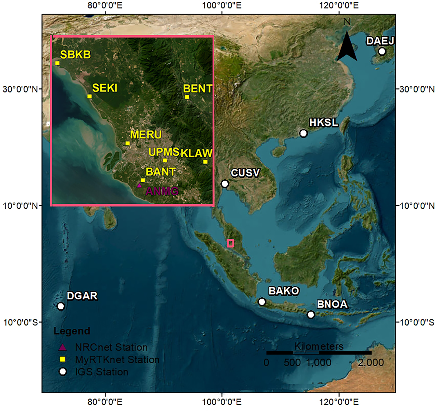
Figure 2: Spatial distribution of GNSS stations

27 GACOS ZTD (Generic Atmospheric Correction Online Service for InSAR zenith total delay) maps corresponding to the SAR acquisition dates were downloaded from the website (http://www.gacos.net) [15]. GACOS tropospheric delay maps are provided in grid binary format (4-byte float little endian, naming convention YYYYMMDD.ztd). The data has a spatial resolution of approximately 0.03° (~3 km) and a temporal resolution of 6 h. MATLAB was used to correct atmospheric effects in the InSAR processing and view the results instantly. GACOS utilizes the Iterative Tropospheric Decomposition (ITD) model to distinguish stratified and turbulent signals from total tropospheric delays and produce high spatial resolution zenith total delay maps for InSAR correction and other applications. For each SAR acquisition date, the GACOS data closest in time to the satellite overpass was selected to ensure optimal correction.

3  Methodology

3.1 InSAR Processing Workflow

The Sentinel-1 SAR images were processed using ESA SNAP, StaMPS, and the TRAIN toolbox. The general workflow (Fig. 3) comprised image preparation, interferogram generation, phase unwrapping, atmospheric correction, and deformation time-series analysis. InSAR processing has two parts, which are Differential Interferometric Synthetic Aperture Radar (DInSAR) and Permanent Scatterer Synthetic Aperture Radar (PSInSAR). DInSAR processing is a technique to generate the coherence and interferograms, while PSInSAR is used to generate the deformation map over time [16]. DInSAR used SNAP software to select the master and slave images through baseline estimation. Orbital correction was applied to produce precise orbits of each image. Then the images were co-registered to compute the interferogram and calculate the interferometric coherence, which helps find a stable permanent scatterer pixel. StaMPs export produces the gamma format acceptable in MATLAB software. In MATLAB, StaMPs permanent scatterer (PSInSAR) processing includes the selection of candidate PS points, estimation of phase noise, PS point selection, and the phase unwrapping process [16]. The unwrapping process produces a shift value in the mean LOS velocity and then generates the deformation map over time. The phase error caused by topography, temporal decorrelation and atmospheric disturbance was removed, so the focus will be on the phase changes by ground movement.

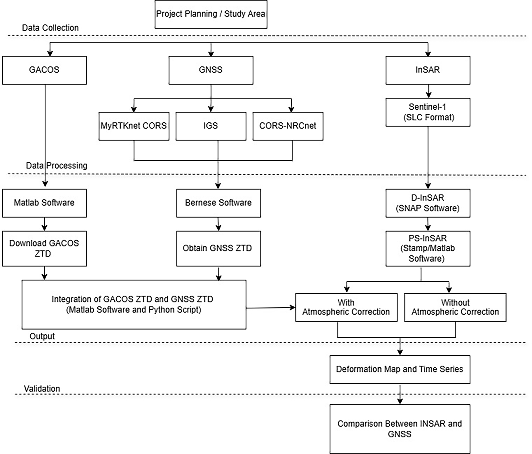
Figure 3: Methodology of InSAR and atmospheric correction

3.2 GNSS Zenith Tropospheric Delay (ZTD) Estimation

To determine ZTD values from MyRTKnet, IGS and CORS-NRCnet GNSS Stations, the Bernese GNSS Software version 5.2 was employed, leveraging its robust algorithms and precise models [17]. ZTD was calculated using GNSS Network Processing (Double-Differencing) processing by incorporating satellite orbital correction, precise satellite clock and receiver information, receiver location error and ionospheric delays, along with meticulous handling of atmospheric effects and instrumental bias [18]. The initial stage of GNSS processing involved preparing the general files (GEN) that will be configured in the Bernese processing system [17]. The GEN files, including PCV_COD.I20, RECEIVER, and SAT_2025.CRX, SATELLITE.I20 and TIDE2000.TPO. Besides that, atmospheric files, clock ephemeris and orbit data were downloaded at the CODE & BSWUSER52 ftp server. Among the files are satellite precise clocks, satellite precise orbits, earth rotation parameter and global ionosphere maps. Processing of GNSS data in Bernese Software involves four stages which are data preparation, data pre-processing, data processing and network adjustment [14]. Fig. 4 shows the processing stages of GNSS data processing in Bernese Software.

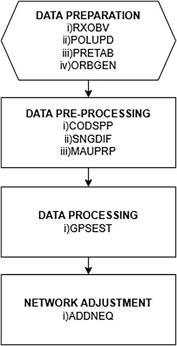
Figure 4: Workflow of GNSS data processing using Bernese

3.3 GNSS–GACOS Integration

The integration of GACOS-derived and GNSS-derived ZTD values was performed using MATLAB, which provided tools for data interpolation, comparison, and visualization. The input data for GNSS data was read from a CSV file containing columns like ‘lon_gnss’, ‘lat_gnss’, and ‘ztd_gnss’, while GACOS ZTD values are read from a binary file (.ztd) with metadata provided in an associated .rsc file. In the grid and interpolation preparation, Latitude and longitude grids are created using metadata from the RSC file and GACOS ZTD data is reshaped into a 2D matrix and matched with its geographic coordinates. At GNSS station locations, ZTD residuals are computed (see Eq. (1)). An empirical variogram is computed using pairwise distances and semivariances of residuals. A theoretical exponential variogram model is fitted to estimate spatial autocorrelation structure (sill, range, nugget). The residuals at the GNSS station are interpolated using Kriging Interpolation over the full spatial grid using the exponential variogram model. Interpolated residuals are added to GACOS ZTD values to generate corrected ZTD estimates. The corrected ZTD values are saved in a new binary file and RSC metadata is copied. Fig. 5 presents a flowchart of the method used for integration of GACOS-derived and GNSS-derived ZTD.

Residual=GNSS ZTD−GACOSZTD(1)

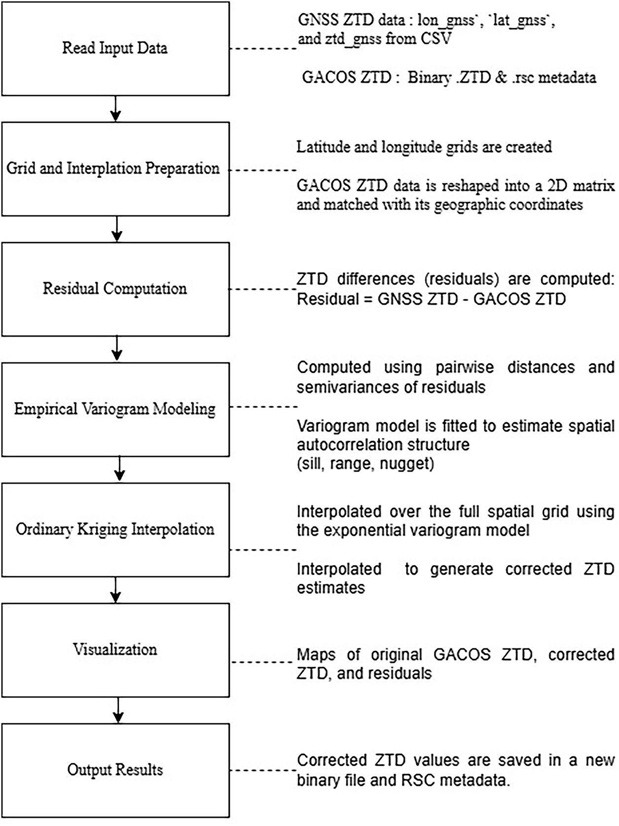
Figure 5: The method for GACOS ZTD and GNSS ZTD integration

The ZTD values obtained through the integration of GACOS and GNSS data were used in conjunction with unwrapped phase results from PSInSAR processing. These inputs were analyzed using the Toolbox for Reducing Atmospheric InSAR Noise (TRAIN). TRAIN developed to correct atmospheric artifacts, particularly ZTD, using meteorological data like GACOS data in this study for the purpose of generating corrected surface deformation measurements [19]. TRAIN processing involves converting ZTD from zenith direction to the Line-of-Sight (LOS) direction of the satellite using local incidence angles and producing spatially variable delay maps matching the SAR image geometry. Finally, TRAIN applies ZTD corrections from GNSS and GACOS to SAR interferograms for improving deformation accuracy.

To validate all the InSAR results, the line of sight (LOS) ellipsoidal height obtained at the MERU MyRTKnet from Bernese 5.2 software processing was analyzed to get the deformation value. The ellipsoidal height is determined by subtracting the reference date from all epochs. Then, the Root Mean Square Error (RMSE) is taken as the evaluation index to compare the accuracy of all InSAR results.

4  Results and Discussions

4.1 Integration of GACOS and GNSS Residual Map

Figs. 6 and 7 present the output of GNSS and GACOS ZTD integration, visualized as residual maps. These maps display the original GACOS ZTD, the corrected GACOS ZTD, and the resulting residual ZTD. The residual maps indicate that the integration is effective, with small residual values suggesting a good agreement between the corrected GACOS and GNSS-derived ZTD.

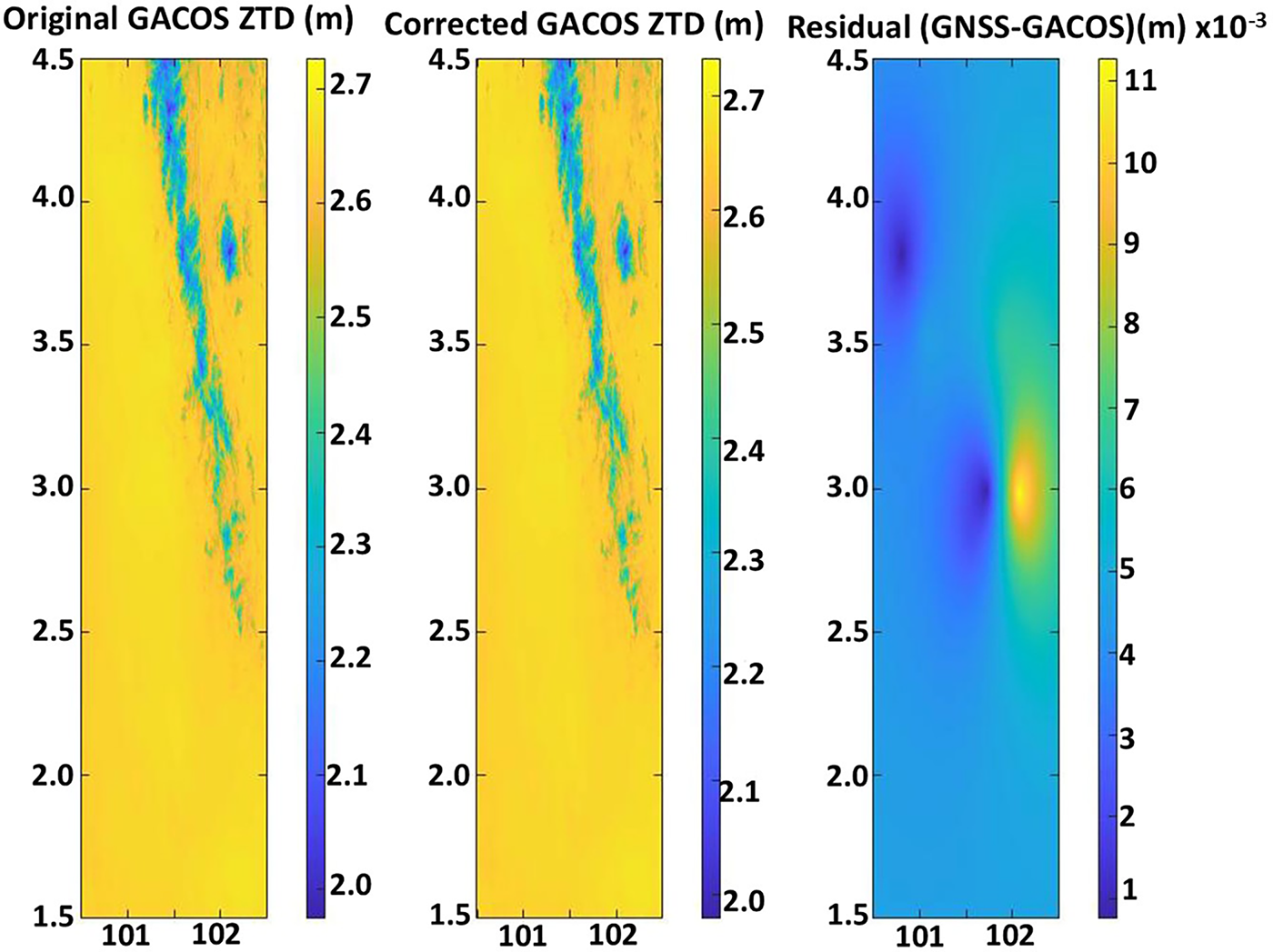
Figure 6: Residual map for GACOS & GNSS ZTD data dated 10 March 2025

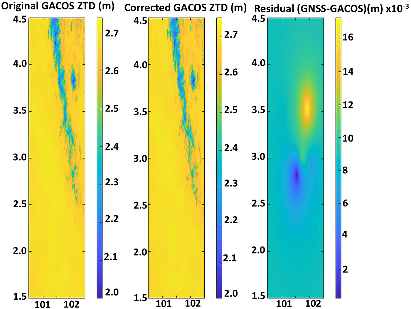
Figure 7: Residual map for GACOS & GNSS ZTD data dated 14 February 2025

4.2 Estimated Ground Deformation

Fig. 8 shows the estimated ground deformation map without applying atmospheric correction, Fig. 9 shows the estimated ground deformation map after accounting for atmospheric correction from GACOS ZTD, while Fig. 10 shows the estimated ground deformation from integration of GNSS and GACOS ZTD. After applying the atmospheric correction, the deformation rates range increased from −14.9 mm/year minimum, 9.1 mm/year maximum to −14.7 mm/year minimum, 9.2 mm/year maximum for GACOS ZTD data and increased to −15.4 mm/year minimum, 9.3 mm/year maximum using integration of GNNS & GACOS ZTD. The deformation rate trend shows that the subsidence rate was somewhat enhanced after the adjustment.

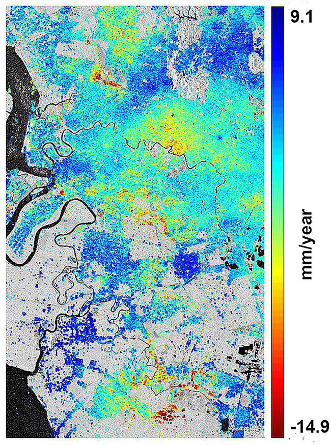
Figure 8: Deformation map without atmospheric correction

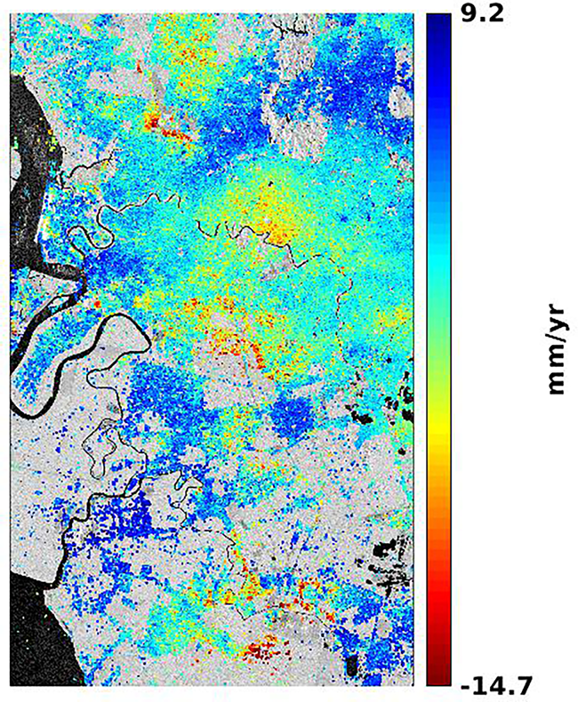
Figure 9: Deformation map with GACOS ZTD

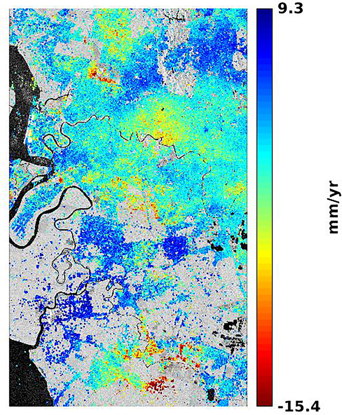
Figure 10: Deformation map after integration of GACOS and GNSS ZTD

Based on the results, the InSAR processing before atmospheric correction (Fig. 8) shows that the most considerable subsidence area is in the northern part of the study area, which is −14.9 mm/year. The most significant uplift is in the southern part, which has a velocity rate of about 9.1 mm/year. After the atmospheric correction using GACOS, the decrease is within 2 mm to a minimum of −14.7 mm/year and a maximum of 9.2 mm/year. If we analyzed based on the colour ramp, the pattern of subsidence area in the northern part decreased to −14.7 mm/year. This shows that atmospheric correction using GACOS ZTD improves the quality of the interferogram since most of the atmospheric influence over the whole study area has been subtracted. After integrating GNSS and GACOS ZTD, the resulting deformation map shows values ranging from −15.4 to 9.3 mm/year, indicating only minor differences compared to the deformation map generated using GACOS ZTD alone. It shows that GNSS measurements cannot effectively reduce atmospheric error since the precision of interpolated water vapour is limited due to the sparse distribution of GPS stations [20]. In addition, the accuracy of the interpolated atmospheric error at the InSAR PS pixel level is dependent on the spatial density of the GNSS stations.

4.3 Deformation Time Series Comparison

Fig. 11 shows a graph visualizing the comparison between reference deformation MyRTKnet (MERU Station) with InSAR without applying atmospheric correction, atmospheric correction from GACOS ZTD and deformation map after integration of GACOS and GNSS ZTD. The master/reference InSAR image and reference date of deformation MyRTKnet was chosen to show the “zero deformation” of temporal resolution between all processing techniques. The deformation map after integration of GACOS and GNSS ZTD gave ground deformation values that were closer to the reference ground deformation (MyRTKnet MERU).

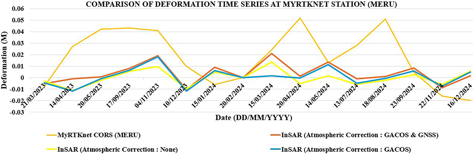
Figure 11: Deformation time series comparison (MyRTKnet MERU Station) and InSAR

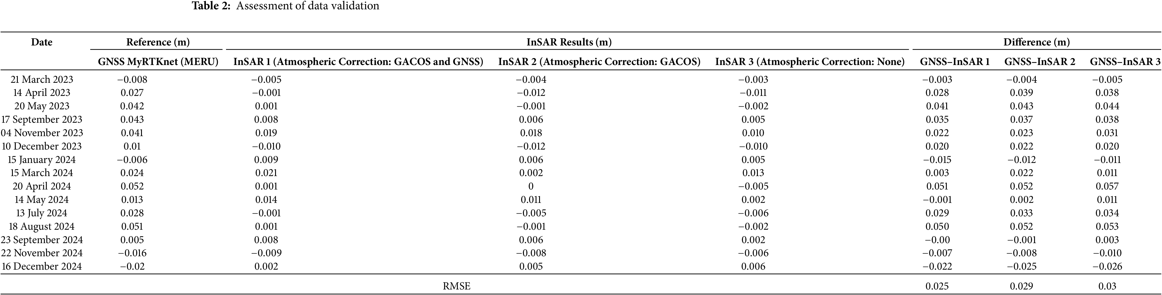
Table 2 above shows the assessment of data validation between the reference deformation MyRTKnet and InSAR processing. The Root Mean Square Error (RMSE) is taken as the evaluation index, and the RMSE value was 0.025 after comparison between reference deformation and integration of GACOS and GNSS ZTD, 0.029 for RMSE atmospheric correction with GACOS ZTD and 0.03 without applying atmospheric correction. The lowest RMSE is 0.025 for comparison between reference deformation and integration of GACOS and GNSS ZTD, which means the best accuracy compared to others. This reduction in RMSE confirms the positive impact of atmospheric correction on deformation accuracy.

The deformation rate was improved after using the atmospheric correction technique, but it still has low accuracy compared to the GNSS reference deformation. The discrepancies observed between GNSS and InSAR-derived deformation values stem from different measurement geometries and atmospheric delay residue. GNSS measures 3D displacements (east, north, and vertical) at discrete points, while InSAR observes displacement over a spatially continuous area along the satellite’s line-of-sight (LOS) direction. The InSAR observation combines both vertical and horizontal movement. However, this study just focuses on the vertical direction of land deformation. Horizontal displacement components are considered minimal and do not significantly affect the subsidence analysis. This means InSAR may miss horizontal displacements perpendicular to LOS. Besides that, using high-resolution weather data like ERA5 may increase InSAR measurements since InSAR is highly sensitive to atmospheric effects [21]. Furthermore, the possible correction effect is still limited by the accuracy of the turbulence data in the GACOS product.

5  Conclusion

This study demonstrates the effectiveness of integrating GNSS and GACOS data to correct atmospheric delays in Sentinel-1 InSAR-based land subsidence monitoring over Banting, Selangor. GACOS correction alone reduced large-scale atmospheric artefacts, improving deformation consistency. GNSS integration further refined local delay patterns, yielding the lowest RMSE (0.025 m) against reference GNSS data. The combined method successfully delineated subsidence zones ranging from −15.4−1 to +9.3 mm year−1. The synergy between GNSS and GACOS provides a practical and precise approach for atmospheric correction in humid tropical environments, enhancing the reliability of InSAR-derived deformation results. Future research should explore real-time implementation and the incorporation of regional numerical weather models to achieve even higher temporal resolution.

Acknowledgement: The authors would like to express their sincere appreciation to the Malaysian Space Agency (MYSA), the Department of Survey and Mapping Malaysia (DSMM) and the International GNSS Service (IGS) for providing access to the GNSS datasets used in this research.

Funding Statement: This research was funded by the Ministry of Higher Education Malaysia (MOHE) through the Fundamental Research Grant Scheme (FRGS/1/2021/WAB07/UiTM/02/1). Additional support was provided by the Land Surveyors Board Malaysia (http://www.ljt.org.my), who generously sponsored the conference registration fee.

Author Contributions: The authors confirm contribution to the paper as follows: Conceptualization, Amir Sharifuddin Ab Latip and Zulkiflee Abd Latif; methodology, Mohd Hakimi Abdul Rahman; validation, Mohd Fikri Razali and Nur Azlina Hariffin; formal analysis, Amir Sharifuddin Ab Latip; investigation, Zulkiflee Abd Latif; resources, Siti Balqis Mohd Tun; data curation, Mohd Fikri Razali; writing—original draft preparation, Amir Sharifuddin Ab Latip; writing—review and editing, Mohd Hakimi Abdul Rahman; visualization, Nur Azlina Hariffin; supervision, Mohd Fikri Razali; project administration, Mohd Hakimi Abdul Rahman; funding acquisition, Zulkiflee Abd Latif. All authors reviewed the results and approved the final version of the manuscript.

Availability of Data and Materials: The data that support the findings of this study are openly available in Copernicus Browser at https://browser.dataspace.copernicus.eu/ (accessed on 01 July 2025), Crustal Dynamics Data Information System (CDDIS) at https://cddis.nasa.gov/archive/gnss/data/daily/ (accessed on 01 January 2025) and GACOS ZTD delay map at http://www.gacos.net.

Ethics Approval: Not applicable.

Conflicts of Interest: The authors declare no conflicts of interest to report regarding the present study.

References

1. Davydzenka T, Tahmasebi P, Shokri N. Unveiling the global extent of land subsidence: the sinking crisis. Geophys Res Lett. 2024;51(4):1–11. doi:10.1029/2023GL104497. [Google Scholar] [CrossRef]

2. Lyu HM, Shen SL, Zhou A, Yang J. Risk assessment of mega-city infrastructures related to land subsidence using improved trapezoidal FAHP. Sci Total Environ. 2020;717(2):135310. doi:10.1016/j.scitotenv.2019.135310. [Google Scholar] [PubMed] [CrossRef]

3. Bagheri-Gavkosh M, Hosseini SM, Ataie-Ashtiani B, Sohani Y, Ebrahimian H, Morovat F, et al. Land subsidence: a global challenge. Sci Total Environ. 2021;778(6):146193. doi:10.1016/j.scitotenv.2021.146193. [Google Scholar] [PubMed] [CrossRef]

4. Zhang Q, Fan H, Qin Y, Zhou Y. Advances in interferometric synthetic aperture radar technology and systems and recent advances in Chinese SAR missions. Sensors. 2025;25(15):4616. doi:10.3390/s25154616. [Google Scholar] [PubMed] [CrossRef]

5. Hashim H, Suhatril M, Hashim R. Assessment of liquefaction hazard along shoreline areas of Peninsular Malaysia. Geomat Nat Hazards Risk. 2017;8(2):1853–68. doi:10.1080/19475705.2017.1391882. [Google Scholar] [CrossRef]

6. Ulma T, Anjasmara IM, Hayati N. Atmospheric phase delay correction of PS-InSAR to monitor land subsidence in Surabaya. IOP Conf Ser Earth Environ Sci. 2021;936:12033. [Google Scholar]

7. Sapucci LF, Machado LAT, de Souza EM, Campos TB. Global positioning system precipitable water vapour (GPS-PWV) jumps before intense rain events: a potential application to nowcasting. Meteor Appl. 2019;26(1):49–63. doi:10.1002/met.1735. [Google Scholar] [CrossRef]

8. Jin S, Komjathy A. GNSS reflectometry and remote sensing: new objectives and results. Adv Space Res. 2010;46(2):111–7. doi:10.1016/j.asr.2010.01.014. [Google Scholar] [CrossRef]

9. Hutabarat LE, Rainaldo D, Ilyas T, Prakoso WA. Site characterization of marine clay consolidation ratio on Kamal Muara Area, Northern Jakarta. IOP Conf Ser Earth Environ Sci. 2019;258:12020. doi:10.1088/1755-1315/258/1/012020. [Google Scholar] [CrossRef]

10. Bernama. Large surface cracks spark Jalan Banting-Klang closure [Internet]. 2020 [cited 2025 Jul 1]. Available from: https://www.malaymail.com/news/malaysia/2020/07/20/jalan-klang-banting-closed-due-to-soil-erosion-sedimentation/1886367. [Google Scholar]

11. Bernama. Excavator driver crushed to death in landslide [Internet]. 2024 [cited 2025 Jul 1]. Available from: https://www.bernama.com/en/news.php?id=2276672. [Google Scholar]

12. Jumaah HJ, Rashid AA, Saleh SA, Jumaah SJ. Deep neural remote sensing and Sentinel-2 satellite image processing of Kirkuk City, Iraq for sustainable prospective. J Opt Photonics Res. 2025;2(3):172–80. doi:10.47852/bonviewjopr42022920. [Google Scholar] [CrossRef]

13. Ab Latip AS, Ansar AM, Din AH, Balogun AL. Correcting atmospheric effects on the InSAR measurements using GPS data. IOP Conf Ser Earth Environ Sci. 2022;1067:12043. doi:10.1088/1755-1315/1067/1/012043. [Google Scholar] [CrossRef]

14. Meng Chan L, Setan H, Othman R. Continuous deformation monitoring using GPS and robust method: iSKANDARNET [Internet]. 2011 [cited 2025 Jul 1]. Available from: https://www.researchgate.net/publication/351122176. [Google Scholar]

15. Zhu S, Zuo X, Shi K, Li Y, Guo S, Li C. Surface subsidence monitoring in Kunming City with time-series InSAR and GNSS. Appl Sci. 2022;12(24):12752. doi:10.3390/app122412752. [Google Scholar] [CrossRef]

16. Hooper A, Bekaert D, Hussain E, Spaans K. StaMPS/MTI manual version 4.1b [Internet]. 2018 [cited 2025 Jul 1]. Available from: https://homepages.see.leeds.ac.uk/~earahoo/stamps/StaMPS_Manual_v4.1b1.pdf. [Google Scholar]

17. Dach R, Lutz S, Walser P, Fridez P. Bernese GNSS software version 5.2. Bern, Switzerland: Astronomical Institute, University of Bern; 2015. doi:10.7892/boris.72297. [Google Scholar] [CrossRef]

18. Sakic P, Männel B, Bradke M, Ballu V, de Chabalier JB, Lemarchand A. Estimation of lesser Antilles vertical velocity fields using a GNSS-PPP software comparison. In: Beyond 100: the next century in geodesy. Cham, Switzerland: Springer International Publishing; 2020. p. 169–80. doi:10.1007/1345_2020_101. [Google Scholar] [CrossRef]

19. Bekaert DPS, Walters RJ, Wright TJ, Hooper AJ, Parker DJ. Statistical comparison of InSAR tropospheric correction techniques. Remote Sens Environ. 2015;170:40–7. doi:10.1016/j.rse.2015.08.035. [Google Scholar] [CrossRef]

20. Thundathil R, Zus F, Dick G, Wickert J. Assimilation of GNSS zenith delays and tropospheric gradients: a sensitivity study utilizing sparse and dense station networks. EGUsphere. 2025;1-24. doi:10.5194/egusphere-2025-19. [Google Scholar] [CrossRef]

21. Hu Z, Mallorquí JJ. An accurate method to correct atmospheric phase delay for InSAR with the ERA5 global atmospheric model. Remote Sens. 2019;11(17):1969. doi:10.3390/rs11171969. [Google Scholar] [CrossRef]