Big Data Analytics Using Graph Signal Processing

1  Introduction

Data all around us is large. The analysis and the processing of large data sets pose a significant challenge [1,2]. A large amount of data is collected and studied in various disciplines such as; natural sciences, engineering, complex networks, social networks, etc. Extracting valuable information from big data sources is a difficult task [3,4]. Data are often structured in a social network and we need to consider the structure behind this data [5]. Generally, the social network is comprised of various elements such as; people (known as actors), and the relationship between these people are known as edges [5]. Fig. 1 shows the example of a social network where nodes represent people and edges show the relations between nodes. For instance, this graph exhibits the node-to-node relation across the network. A graph is an abstract data type and signifies the relations. The graph can be considered a data model, and hence it demonstrates the complex interactions between them. The structural objects are mainly composed of links and nodes. The network grows in size and the complexity increases. Therefore, our ability to analyze it using the current state-of-the-art methods is at risk of failing to keep space. To overcome this problem, our study presented a framework using Graph Signal Processing (GSP) for big data analytics [6]. The GSP is an emerging field that aims to extend the concepts of classical digital signal processing (DSP) to graphs [7]. It is a fast-growing field where classical signal processing tools developed in the Euclidean domain have been generalized to irregular domains such as graphs [8]. In recent years several GSP methods have been developed to process the signals [9]. There is limited work has been reported in the literature for GSP and the big data domain.

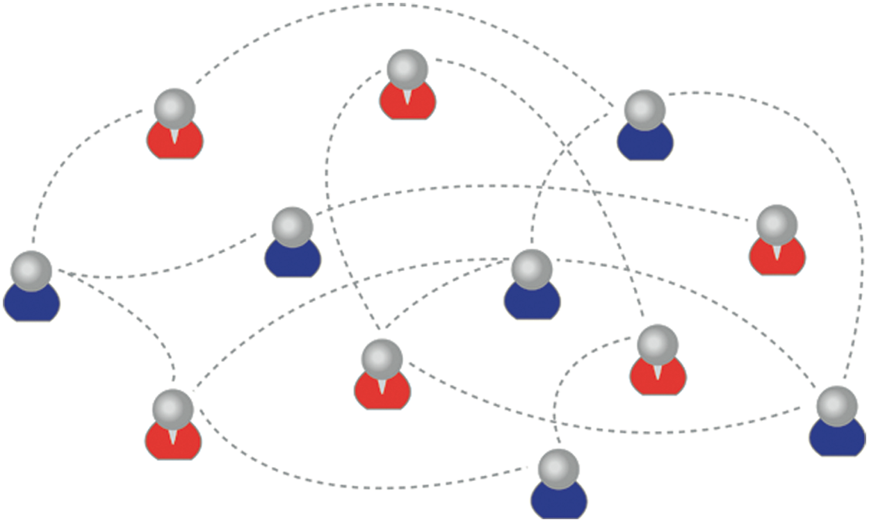
Figure 1: Social network data

1.1 Motivation for Our Study

Data collected from engineering and physical applications in fields like cell biology, social activity, and the economy are becoming larger and more complex. In many cases, the data is analyzed manually or by traditional methods that extract only superficial information and can lead to non-reproducible conclusions. Thus, the primary motivation for this study is to find alternative methods and tools for data analysis. This article considers the use of GSP as a methodology for big data analysis. We discuss the fundamentals of signal processing, such as filtering and frequency analysis, etc. The presented methodology introduces elements of high-performance computing to digital signal processing and offers a structured approach to the development of data analysis tools for large data volumes. The key contributions of our study are given below.

1.2 Contributions of This Study

•   In this review study, we have highlighted the importance of GSP for the processing of large datasets from the perspective of big data. We have discussed, basic graph signal processing methods, such as; frequency analysis, filtering and Laplace operator, etc.

•   We have demonstrated how we can generate a noisy graph signal and later apply it to a large-scale network. By using applying filtering to this signal, we thoroughly demonstrated that graph filtration is efficient for the removal of noise.

•   We have discussed the challenges of GSP for Big Data.

The benefits of our study are as given below.

•   It will be helpful to the researchers who wish to learn the alternative methods of processing large-scale graphs.

•   This study is helpful to researchers who want to understand the structural properties of a graph.

The rest of the paper is organized as follows. Section II provides related work. In section III, we have discussed the fundamentals of signal processing methods such as; filtering, frequency and shift operator, Fourier transform, etc. Section IV offers the advantages and challenges. Section V describes the conclusion of this study.

2  Related Work

The processing of large-scale data or big data is a difficult task [10]. Thus, To solve that problem, Sandryhaila et al. [1] discussed the representation and the processing of massive datasets using irregular graphs. They discussed the necessity and the importance of GSP and also discussed a few graph-based models. In the end, they highlighted various challenges to big data. Ortega et al. in [11], discussed a survey of GSP. In this study, they have presented different tools for the processing of data using an irregular graph. They have discussed different examples by using several applications such as image processing, machine learning, biological sciences, etc. They had summarized a few GSP tools for the sampling of data. Similarly, Stankovic et al. in [12], presented a middleware language using graph signals. They have defined various fundamental concepts in DSP, such as; parameter estimation and filter design. They illustrated by using examples that these are very useful in the processing of graph data. Poor et al. in [13], discussed the issues of signal processing for social networks. In this paper, they had discussed various challenges. The first challenge is size and the complexity. When the network grows this problem occurs. In this regard, how to analyze the network using current signal processing methods is at high risk. Because they do not offer space. The second challenge is the involvement of multi-agents. The third challenge is the analysis and the visualizing of big data by using social networks. Although, this study presents a brief overview of signal processing. But, the authors did not discuss possible solutions to handle the above-discussed challenges. Papalexakis et al. in [14], present social network analysis (SNA) using signal processing methods using tensors. In this study, they had proposed a model, with the capability to analyze the location-based social networks (LBSNs) using tensors and tensor decomposition. Also, they have used signal processing methods to identify the most frequent hidden user communities. Vinciarelli et al. present social signal processing (SSP) in [15]. In this study, they had defined a new term called a social signal. The social signal is one aspect of social intelligence. It is a truth of human intelligence that is very necessary for success in life. It is an ability to recognize the human’s social signal and predict social behavior. Social behavior includes politeness and talking. Also, this study focused on the needs of next-generation computing which includes the essence of social intelligence. To the end, they had performed a comparison of various past efforts in solving these problems by using a computer. Pentland et al. in [16], discussed social signal methods derived from classical signal processing. They clarify an advanced social signaling method, which allows the information to be smoothly integrated into a group. Social signaling includes a signal of interest (SoI), friendliness, determination, and attitudes towards a social situation. They have discussed various issues and the challenges in this newly derived area. In the end, they had demonstrated that by using social signal processing, we can easily predict human behavior.

3  Graph Signal Processing

We have divided this section into different sub-sections. At first, we discussed the basis of graphs, DSP, definition, notation, and the concepts derived from DSP. Then we have discussed the shift operator and the Graph Fourier transform (GFT). The filtering and the advantages have been discussed in subsequent sections. Finally, we have presented an example application by employing all these concepts.

3.1 The Basis of Graph Signal Processing (GSP)

GSP is a newly derived research area and has been rooted in DSP and graph theory [17]. The graph is the collection of nodes and edges. A graph acts as a wiring network that holds the relationship between nodes. The application domain of GSP is brain imaging, transport, and social networks. The graph data is defined as; G=(V,E,WE) where V,E and WE denotes the group of nodes, edges called connections, and the edge weight especially. It is noted that we assume that our graph is undirected. In GSP a signal can be defined over a graph. A graph signal is represented as a vector. The signal is represented by S on a graph.

s:V→RN(1)

The graph structure data provides basic node properties and the network structure. This information is very useful in solving various difficult tasks. There are various examples are available: such as; In Neuroscience, the network is referred to as a graph. The connected edges present different functional regions. Each region is presented by its location area, such as; sensory association, etc. Fig. 2 presents a simple graph signal example. In this figure, we examine that on the left hand a graph containing vertices, V1toV9 were described. The vector RN presents positive and negative values. The +Ve value is represented in red color and the blue color demonstrates -Ve values. On the right-hand side, the graph function is displayed and it shows both positive and negative values. There are many different ways to represent a signal in the spatial domain. Fig. 3 a) illustrates two of them: a 3D representation where signal values are depicted as bars with corresponding heights and Fig. 3 b) depicts signal values as color intensities.

Figure 2: A simple graph signal

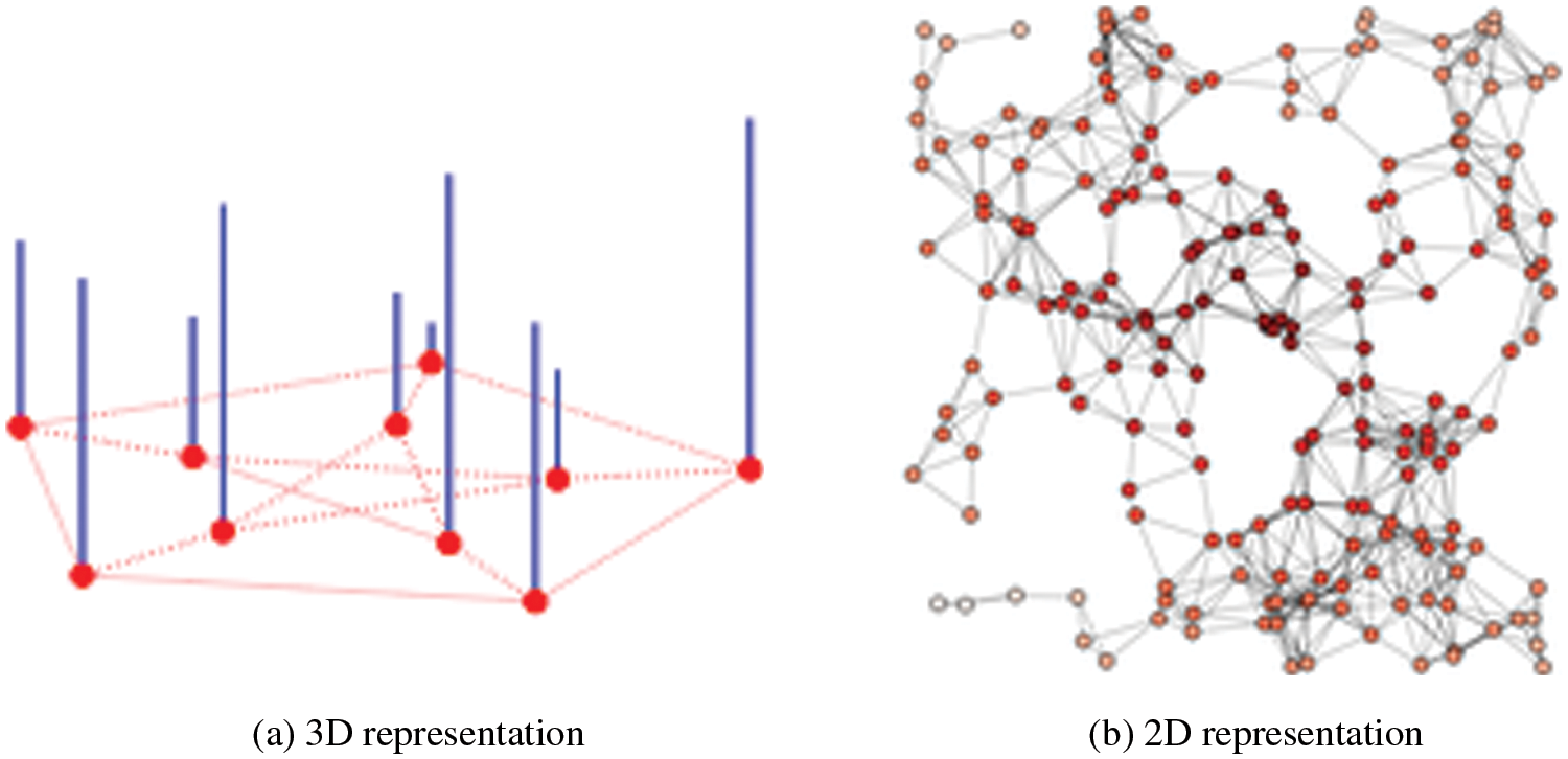
Figure 3: (a) 3D representation (b) 2D representation

3.2 The Shift Operator in Signal Processing

In DSP generally, the signals are displayed in a spectral domain or time domain [18]. The spectral domain has many advantages, such as filtering, effective sampling, information dimensionality, etc [19]. In the spectral domain, we need to apply Fourier transforms (FT), Laplace transforms (LT), or wavelets. In DSP one of the popular transforms is known as; the z-transform [20]. It essentially expands a signal S=RN×1 to a scaled power series.

Z(s[n])=∑n=0N−1⁡SnZ−n(2)

The Z-transform is important, and the fundamental building block used in modern signal processing. The basic polynomial form term is Z−1. It is also referred to as shift or time delay. To make it clearer, we have used, sift to filter the delta function, i.e., δ|n−k|. It has a signal of zeros with 1. The power series of shifts is achieved by multiplying the z-transform of δ|n| with the z- transform filter.

Z(δ|n|)=∑k=0N−1⁡Z(δ|n−k|Z−k1.z0+1.z0+=z0=1)(3)

hshift(z)=∑n=0N−1⁡hnz−n=1.z−1+1.z−2+…=z−1(4)

Finally, when we apply the filter it would result in

Z(δ|n|).hshift(z)=z0.z−1+0.z−2+…=z−1=Z(δ|n|)(5)

In this equation, we examine that it appears to sift the signal by using one sample. Therefore, we would like to have a shift graph operator with the equivalent properties.

3.3 The Shift Operator in Graphs

In the GSP domain, we assume a time-domain signal. In Fig. 4, we can see a graph structure and, in this graph, periodic time-series signal s is shown;

s=[x0,x1−−−−−xN−1]T(6)

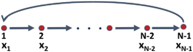
Figure 4: Time graph

It holds a graph-based structure of a directed cyclic graph. Where s[n]=s[n+N]. It seems that the signal can be sifted by multiplying it with A∈R|V|×|V|.

The cyclic shift matrix S.t.sshifted = A.S when

A=(001100010)(7)

We can see that the cyclic graph operators are precisely called the “Adjacency matrix” as shown in the time domain signal. In a time-domain signal, the cyclic shift operator is precisely defined as an adjacency matrix. The matrix is symmetric and the entries are equal to zero and one. In this matrix if aij=0, means that there is no link connecting node i and node j. The time-domain signal defines the unidirectional flow of information in a graph and also supplies time context to the set of graph signal values [21]. We noticed that in this linear operation the substituting value of a node and the neighbor will be performed. This fact leads to highlight the one most important property of shift operator. Simply, it behaves like a local operator in the vertex domain. There are numerous variations of the graph shift matrix have been proposed. The popular choice is known as the Laplace operator or non-normalized combinational graph Laplacian.

L=D−AAnd symmetric normalized Laplacian, i.e.

L=D12.D12,whereDisthedegreematrix.

Dij={∑j=1|V|aijifi−j0else(8)

The graph Laplacian can be considered as a low pass filter. Or simply it is a difference between the signals of a node to the signals of its neighbors.

3.4 Graph Frequencies

In this section, we have discussed the frequencies and their notations. Generally, in DSP the frequencies are discussed in the time domain. These frequencies are sinusoid oscillating at low to high rates. In GSP, there are two types of frequencies used, i.e., low and high [22]. These frequencies define the number of change values between the connected components of a graph. The change is measured in terms of graph total variation. The variation measures the difference between the graph signal and the shifted version. The spectral component or graph frequency is obtained via a method named spectral decomposition. In this method, a graphical structure is decomposed into the N distinct Eigenvalues. This method is very helpful in the estimation of frequencies or the graph spectrum. These are invariant to node permutations. This important property defines an important constraint for graph learning tasks. It differs from DSP, where the transform is not universal. For example; Graph Laplacian shift L is a real symmetric matrix and hence it can be decomposed into the quadratic form:

L=x∧LT(9)

In this equation; the columns of x denote the eigenvector and ∧ is a diagonal matrix and ⋋ is the relative power of the ith eigenvector. In proof of concept (POC), the Eigenvector xi can be considered as a Fourier basic function, ejwr and ⋋i is the frequency of this function. If the frequency is lower, then the signal is more smooth or more regular. Fig. 5 presents the graph frequencies. In this graph, we can easily observe the effect of graph Laplacian. Four different graphs were formed and each graph has positive and negative signals. We noticed that both signals depend upon the value of ⋋i. If we use the value then, we are getting only –Ve signal and if we increase the ⋋i value, then we are getting both positive and negative values. The Eigenvector of a graph Laplacian is used to define the analogous Graph Fourier transform (GFT) of a signal s over graph Laplacian L.

FL(s)=[X1Ts,X1Ts,…….,XN−1Ts]s.t.XiLXiT=⋋i(10)

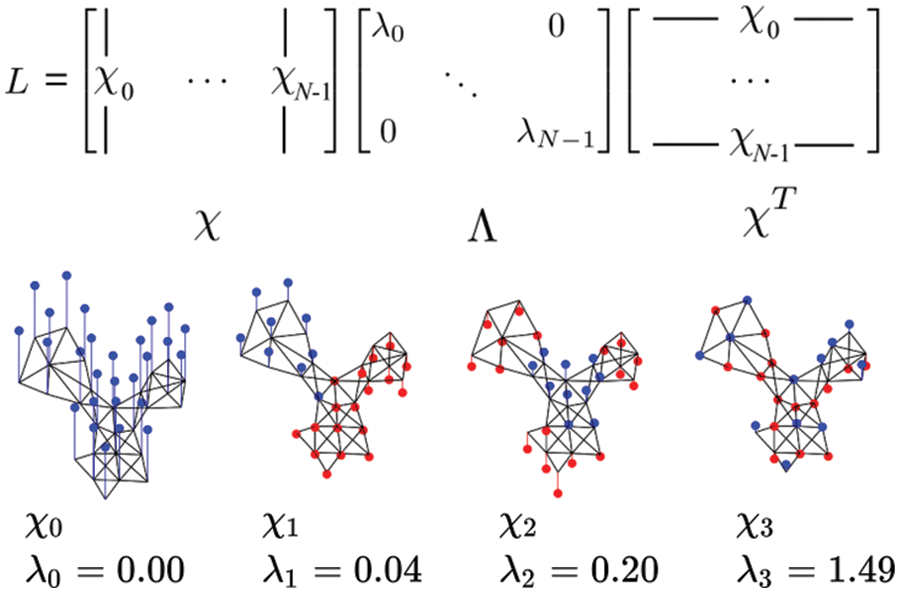
Figure 5: Visual example of graph frequencies

The compassion of Fourier transform (CFT) in the time domain and graph domain is given below.

DSP−Fw(s)=∫(ejwt)∗s(t)dt(11)

GSP−Fl(s)=∑iXl∗(i)s(i)di(12)

3.5 Filtering Graph Signals

The filtering process is used to remove noise from frequencies. Primarily, it allows us to isolate the individual frequencies, and hence the noise is removed from the signal [1]. The term GFT is used for the filtering of graph signals. It uses a convolution theorem to perform spectral filtering. According to DSP, under suitable conditions, the Fourier transform of a convolution of two signals is the pairwise product of their Fourier transform.

We can filter on an input signal:

sout=H.sin=Xh(∧)xTsin=X.diag[h(⋋0),……..,h(⋋N−1)].sin

It is easier to identify the classic time-domain equations when we are looking for non-matrix equations.

DSP−sout(t)=∫Sin(w)h∧(w)ejwt=(Sin∗h)(t)(13)

DSP−sout(i)=∑l=0N−1⁡Sin(⋋e)h∧(⋋e)Xe(i)(14)

This filtering process is quite expensive. In the next section, we design a heat filter and then apply it to real-world traffic data for the computation of distance in the network.

The Polynomial approximation for localized graph filters is intended for saving computations, and specifically reducing the Eigen decomposition and multiplication. There are several popular approximations in GSP such as; Minmax, Meyer, Least Squares (LS), Lanczos method, etc. The most popular approximation is known as the Chebyshev expansion(CE). It is highly efficient due to the recursive formulation of the filter.

h∧(⋋e)=∑k=0k−1⁡akTk(∧∼)s.tTk(x)=2xTk−1(x)−Tk−2(x)(15)

3.6 Example Application

As a motivational application of GSP, we consider filtering a Minnesota road network. The road traffic data has been collected from a real-world dataset; i.e., Minnesota road network. Fig. 6 presents the Minnesota road map graph using geospatial context and Graph spring layout. This dataset includes 2642 nodes (intersections) and 3304 links (roads). For instance, we have used Network X for simulation and experimentation purposes. The Network X [23], is a popular python-based package used for the graphs. We begin by visualizing the graph with a geospatial context. Every node is located according to its coordinate. The graph is constructed by using the intersections as nodes and the roads as undirected edges. The network structure includes information only about the graph edges and is blind to the geospatial location of the node. This enables us to do very simple and visible geo-spatial manipulation, which aligns with the node’s location for a better demonstration. Here we visualize the graph with and without the geospatial context. Next, we create a noisy signal based on the distance from the dense part of Minnesota. We have used coordinates for that graph, i.e., (−93.2,45). And have used a nonlinear cutoff value for sin>2 to further localize the signal. If the value is <2, we can’t get the uniform value and it would affect in terms of non-filtering effect. Fig. 7 presents the Minnesota road graph using a simulated signal where the nodes and edges of Minnesota were shown at the top of the graph. Then we design a heat filter and then visualize it in the spectral domain. The impulse response of this filter is g(x)=exp⁡(−Txλmax). This filter is low pass filter, we choose T=50 because we want to assure the removal of higher noisy frequencies, and we assume that the spectral components that describe the clean signal have very small eigenvalues. Fig. 8 presents the visual effect of the filter frequency response. We visualize the effect of the filter on the noisy signal. Fig. 9 a) presents the actual data before filtering and Fig. 9 b) presents the approximation data using a filtered noisy signal. Now we design the new signal as a combination of some noise. This new signal is shown in Fig. 10. Fig. 11 shows the filtered removal graph. When we compare actual or original graph and filter removal, there are very closer. It seems that the filtering process succeeded.

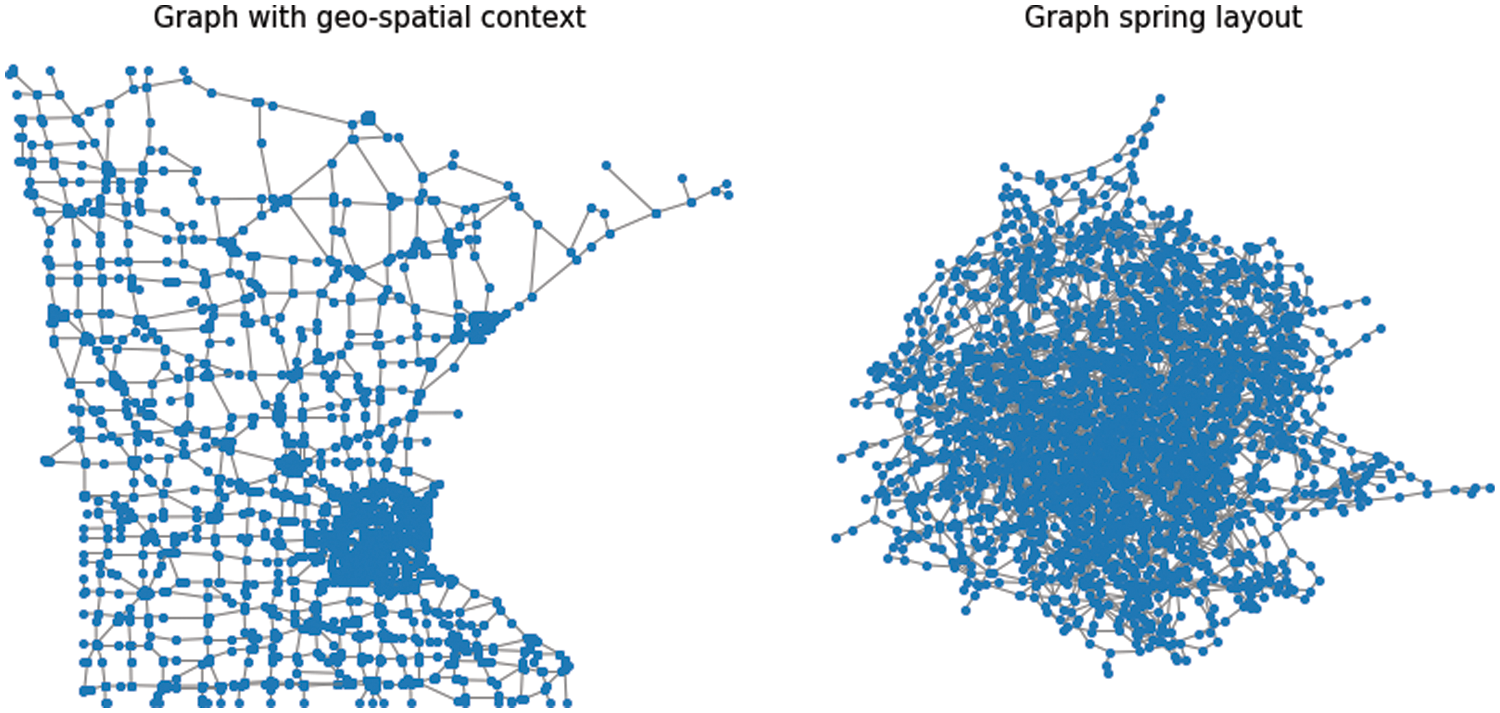
Figure 6: The Graph visualization using geo-spatial context and Graph spring layout

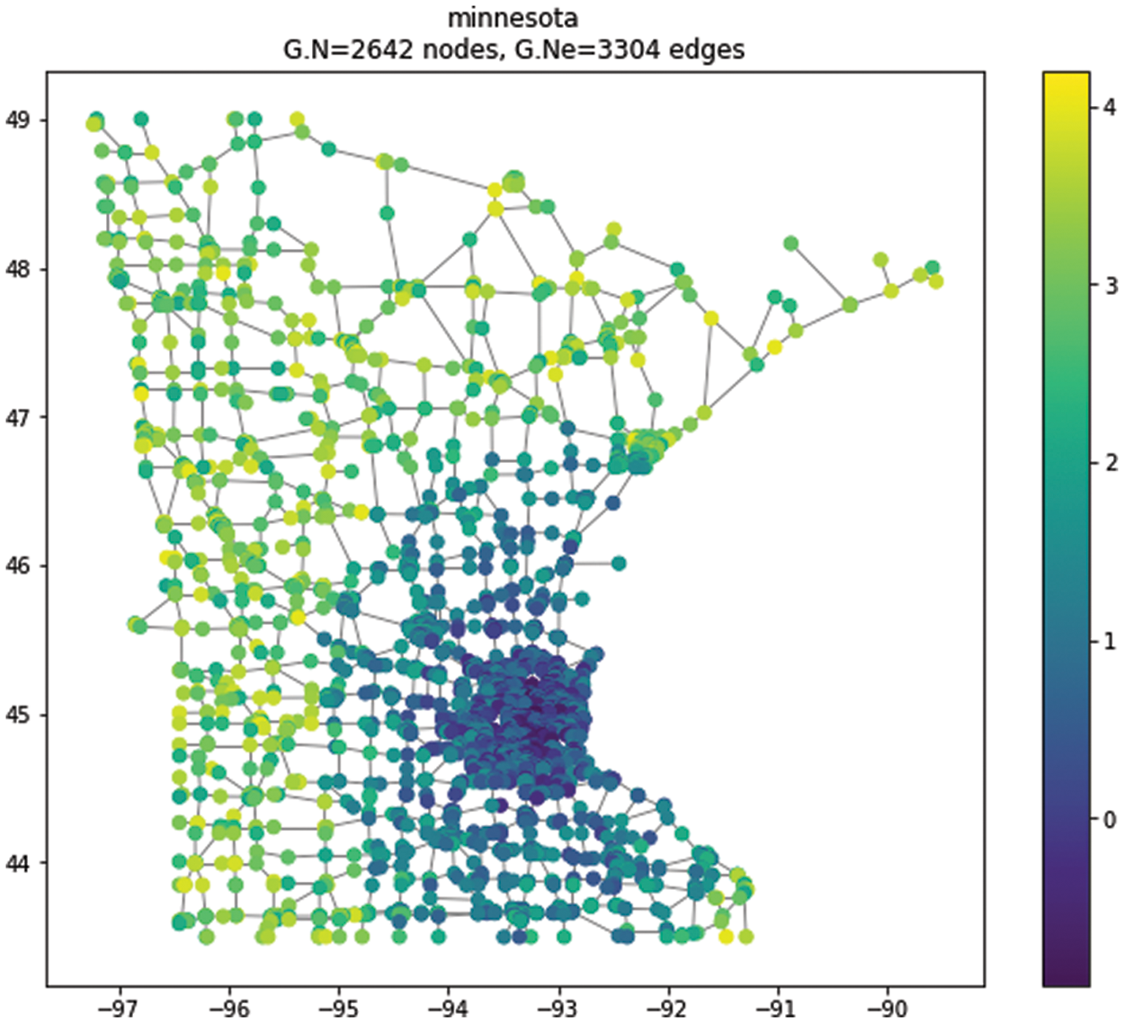
Figure 7: The Minnesota road graph: Noisy signal

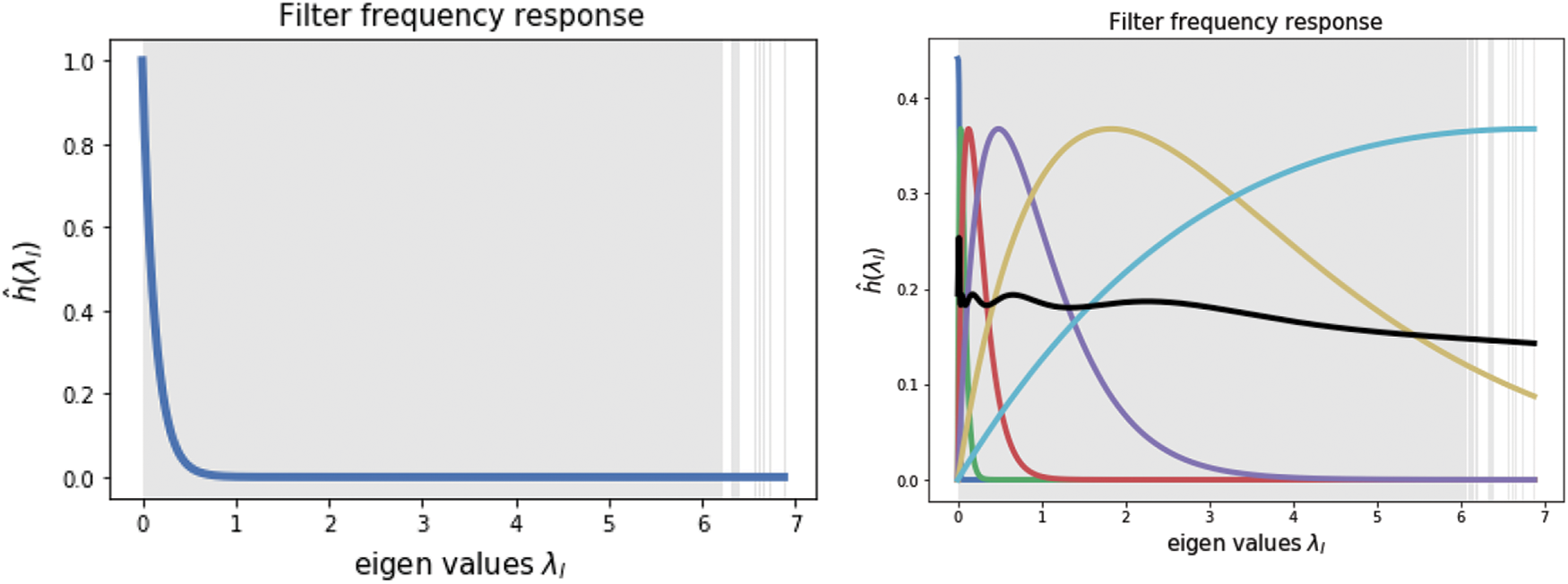
Figure 8: Filter frequency response

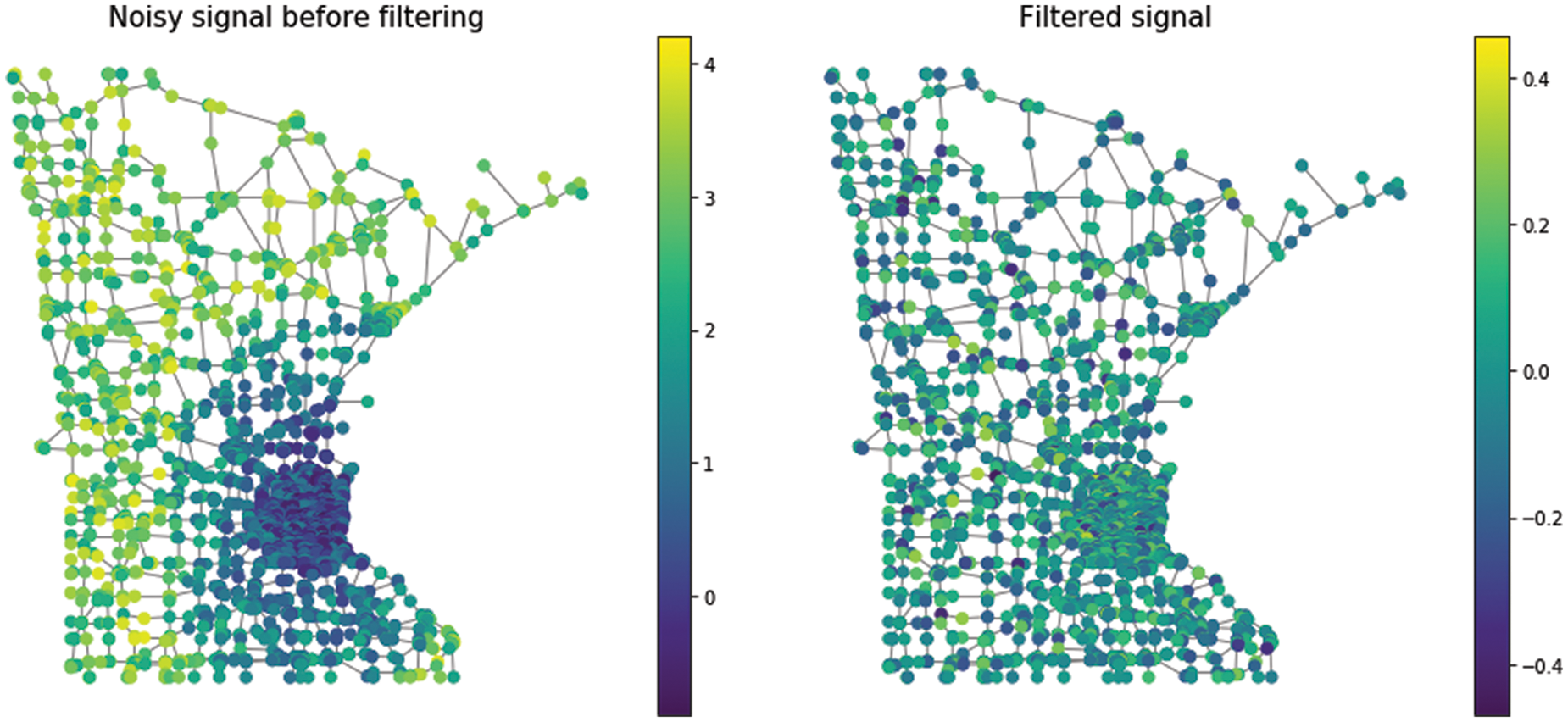
Figure 9: The effect of filter on a noisy signal

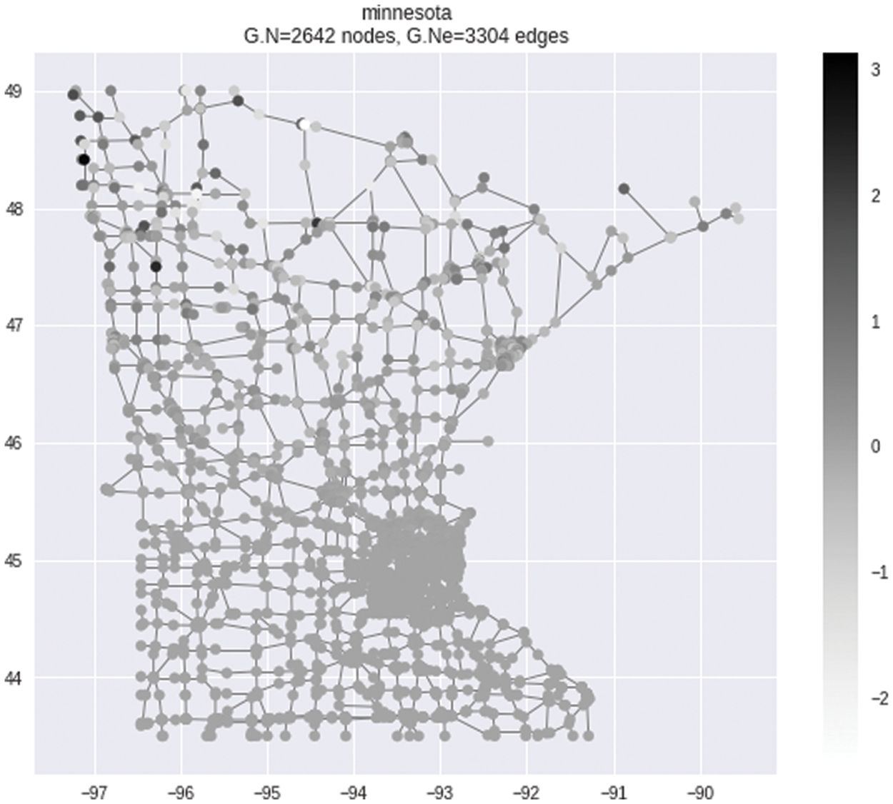
Figure 10: Signal combination of noise

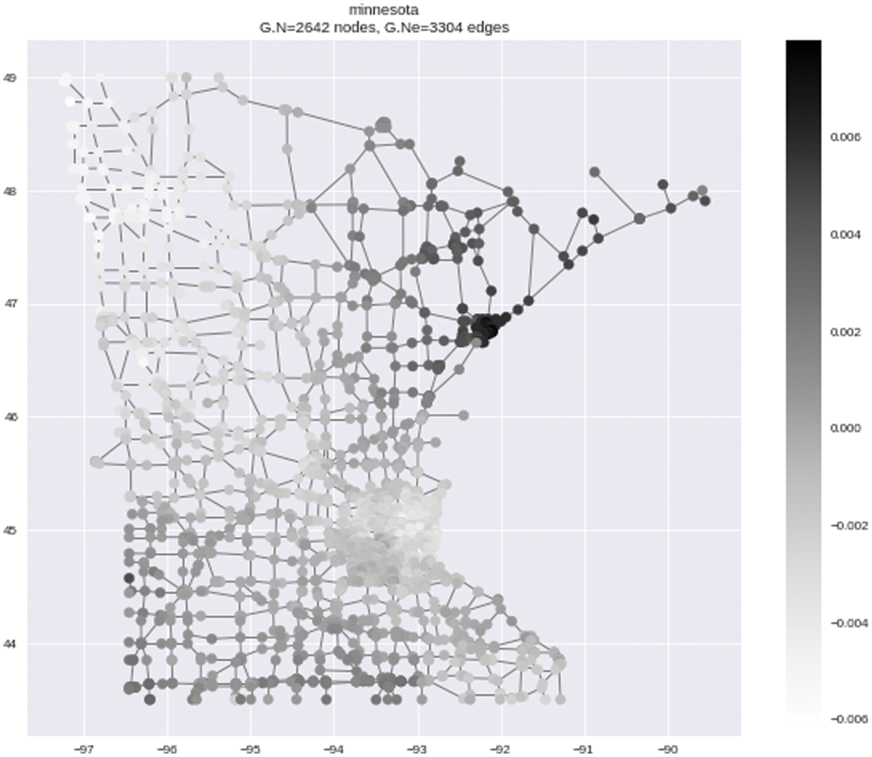
Figure 11: Filter removal

3.7 The Advantages of Digital Signal Processing

Generally, in a large network, the data is presented in the form of a graph and that can be diverse. This challenge is addressed by DSP by demonstrating the data structure with graphs and also quantifying the data into graph signals. The flexible graph structure provides versatile data abstraction for various types of data such as telecom data etc [24]. The graph Laplacian or Laplacian operator could help in finding services of the Internet of things (IoT) [25].

4  Challenges and Issues in this Direction

Current research trends focused on reducing the calculation and the complexity when we are dealing with large graphs. It includes graph segmentation down-sampling, deep learning, multidimensional graph structure, vertex frequency, vertex varying, etc [12]. When the network grows, it increases in size, and at the same time complexity also increases [13]. In that case, the current state-of-the-art models in signal processing are not adequate. Most commonly they have memory and space problems. The analysis, processing, and visualization of “big data” is a very challenging task. The data may be very large. To provide more meaningful information we need to develop more novel machine learning and statistical tools based on algorithmic approaches using GSP and big data.

5  Conclusion

In this article, we have presented a literature review of graph signal processing. First of all, we reviewed the basic concepts of GSP and explained frequency, Fourier transforms, shift operator and graph filter, etc. To address important challenges in Big Data analysis and make implementations of fundamental Digital signal processing (DSP) techniques suitable for large datasets, we considered an example application by using graph filtering. We have created a noisy signal and then applied a filter to this signal. After several rounds of simulation results, we discovered that. It is the same as the original noise-free signal. It means that graph filtering is efficient and can be applied to a large network. In addition, the discussed technique bridges a gap between signal processing, Big Data analysis, and high-performance computing, as well as presents a framework for the development of new methods and tools for the analysis of massive datasets. However, additional research is needed within each application to further understand the best ways to combine GSP tools with existing techniques to achieve significant gains in terms of the metrics of interest for each application.

Acknowledgement: We thank our families and colleagues who provided us with moral support.

Funding Statement: This work was supported in part by Basic Science Research Program through the National Research Foundation of Korea (NRF) funded by the Ministry of Education (NRF-2019R1A2C1006159) and (NRF-2021R1A6A1A03039493), and in part by the 2021 Yeungnam University Research Grant.

Conflicts of Interest: The authors declare that they have no conflicts of interest to report regarding the present study.

References

1. A. Sandryhaila and J. M. F. Moura, “Big data analysis with signal processing on graphs: Representation and processing of massive data sets with irregular structure,” IEEE Signal Processing Magazine, vol. 31, pp. 80–90, 2014. [Google Scholar]
2. L. Stanković, M. Daković and E. Sejdić, “Introduction to graph signal processing,” in Proc. of the Vertex-Frequency Analysis of Graph Signals, Cham, Switzerland, pp. 3–108, 2019. [Google Scholar]
3. L. Atzori, A. Iera, G. Morabito and M. Nitti, “The social internet of things (siot)–when social networks meet the internet of things: Concept, architecture and network characterization,” Computer Networks, vol. 56, pp. 3594–3608, 2012. [Google Scholar]
4. F. Amin, R. Abbasi, A. Rehman and G. S. Choi, “An advanced algorithm for higher network navigation in social internet of things using small-world networks,” Sensors, vol. 19, pp. 2007–2020, 2019. [Google Scholar]
5. F. Amin, A. Ahmad and G. S. Choi, “Community detection and mining using complex networks tools in social internet of things,” in Proc. of the IEEE Region 10 Conf., Jeju, Korea, pp. 2086–2091, 2018. [Google Scholar]
6. S. Ljubiša, P. M. Danilo, D. Miloš and B. Miloš, “Data Analytics on Graphs Part II: Signals on Graphs,” Now Foundations and Trends, vol. 30, pp. 83–98, 2020. [Google Scholar]
7. W. Strauss, “Digital signal processing,” IEEE Signal Processing Magazine, vol. 17, pp. 52–56, 2000. [Google Scholar]
8. W. Hu, J. Pang, X. Liu, D. Tian and C. W. Lin, “Graph signal processing for geometric data and beyond: Theory and applications,” IEEE Transactions on Multimedia, vol. 6, pp. 1, 2021. [Google Scholar]
9. D. I. Shuman, S. K. Narang, P. Frossard and A. Ortega, “The emerging field of signal processing on graphs: Extending high-dimensional data analysis to networks and other irregular domains,” IEEE Signal Processing Magazine, vol. 30, pp. 83–98, 2013. [Google Scholar]
10. S. Chen, Y. C. Eldar and L. Zhao, “Graph unrolling networks: Interpretable neural networks for graph signal denoising,” IEEE Transactions on Signal Processing, vol. 69, pp. 3699–3713, 2021. [Google Scholar]
11. A. Ortega, P. Frossard, J. Kovačević and J. M. Moura, “Graph signal processing: Overview, challenges, and applications,” Proceedings of the IEEE, vol. 106, pp. 808–828, 2018. [Google Scholar]
12. L. Stankovic, D. P. Mandic, M. Dakovic and I. Kisil, “Understanding the basis of graph signal processing via an intuitive example-driven approach,” IEEE Signal Processing Magazine, vol. 36, pp. 133–145, 2019. [Google Scholar]
13. H. V. Poor, K. -C. Chen, V. Krishnamurthy and D. Shah, “Introduction to the issue on signal processing for social networks,” IEEE Journal of Selected Topics in Signal Processing, vol. 8, pp. 511–513, 2014. [Google Scholar]
14. E. E. Papalexakis, K. Pelechrinis and C. Faloutsos, “Location based social network analysis using tensors and signal processing tools,” in Proc. of the Int. Workshop on Computational Advances in Multi-Sensor Adaptive Processing (CAMSAP), Cancun, Mexico, pp. 93–96, 2015. [Google Scholar]
15. A. Vinciarelli, M. Pantic and H. Bourlard, “Social signal processing: Survey of an emerging domain,” Image and Vision Computing, vol. 27, pp. 1743–1759, 2009. [Google Scholar]
16. A. Pentland, “Social signal processing,” IEEE Signal Processing Magazine, vol. 24, pp. 108–111, 2007. [Google Scholar]
17. I. Jabłoński, “Graph signal processing in applications to sensor networks, smart grids, and smart cities,” IEEE Sensors Journal, vol. 17, pp. 7659–7666, 2017. [Google Scholar]
18. J. Miettinen, S. A. Vorobyov and E. Ollila, “Graph error effect in graph signal processing,” in Proc. of the IEEE Int. Conf. on Acoustics, Speech and Signal Processing (ICASSP), Calgary, AB, Canada, pp. 4164–4168, 2018. [Google Scholar]
19. M. Simonovsky and N. Komodakis, “GraphVAE: Towards generation of small graphs using variational autoencoders,” in proc. of the Artificial Neural Networks and Machine Learning, cham, Switzerland, pp. 412–422, 2018. [Google Scholar]
20. L. Rabiner, R. Schafer and C. Rader, “The chirp z-transform algorithm,” IEEE Transactions on Audio and Electroacoustics, vol. 17, pp. 86–92, 2020. [Google Scholar]
21. Y. Tanaka, Y. C. Eldar, A. Ortega and G. Cheung, “Sampling signals on graphs: From theory to applications,” IEEE Signal Processing Magazine, vol. 37, pp. 14–30, 2020. [Google Scholar]
22. X. Dong, D. Thanou, L. Toni, M. Bronstein and P. Frossard, “Graph signal processing for machine learning: A review and new perspectives,” IEEE Signal Processing Magazine, vol. 37, pp. 117–127, 2020. [Google Scholar]
23. A. Hagberg, P. Swart and D. S. Chult, “Exploring network structure, dynamics, and function using networkx,” In Proceeding of the SCIPY, vol. 08, Pasadena, United States, pp. 11–16, 2008. [Google Scholar]
24. F. Amin and G. S. Choi, “Hotspots analysis using cyber-physical-social system for a smart city,” IEEE Access, vol. 8, pp. 1–12, 2020. [Google Scholar]
25. B. Kartal, Y. E. Bayiz and A. Koç, “Graph signal processing: Vertex multiplication,” IEEE Signal Processing Letters, vol. 28, pp. 1270–1274, 2021. [Google Scholar]
Cite This Article
Copyright © 2023 The Author(s). Published by Tech Science Press.
This work is licensed under a Creative Commons Attribution 4.0 International License , which permits unrestricted use, distribution, and reproduction in any medium, provided the original work is properly cited.
Downloads
Citation Tools