Deep Learning-based Environmental Sound Classification Using Feature Fusion and Data Enhancement

1  Introduction

Recently, sound detection has gained attention with a wide range of applications, which include alert systems, wildlife monitoring [1], autonomous cars designation [2], IoT based solution for urban noise detection in smart cities, classification of distinct musical instruments, voice recognition [3,4] etc. It is important to identify the context of the sounds and take appropriate measures to minimize the risks. This indicates the importance of sound detection systems in virtually every aspect, ranging from humans to other living organisms such as plants and animals. The detection of environmental sound is to classify sound classes for recordings or audio clips. The sound classification involves three well-known research areas namely Automatic Speech Recognition (ASR), Music Information Retrieval (MIR), and the ESC. This research focuses on the last area as the ESC audio files are unstructured and have a low Signal to Noise Ratio when compared to ASR and MIR.

Environmental sound contains more variety when compared to speech. Consequently, this variation and the noisy features have made the ESC more challenging than speech detection. In recent years, sound detection has made great progress in the research domain, which can be attributed to the publicly available annotated datasets such as UrbanSound8k (US8K) [5], and ESC version 10 and 50 datasets (ESC-10 & ESC-50) [6]. Another reason is due to the transition from conventional machine learning approach to deep learning approach in the sound classification tasks. Moreover, ESC tasks face various challenges, which makes it hard to experiment. However, one of the major challenges in ESC is that it lacks specific audio scene/structural music signals. Another reason is that the ratio of signals to noise is negligible because of the wide range of distance between the voice generation source and the audio clip recorder when compared with the speech recognition system and musical information retrieval. Thus, the aforementioned problems lead to the difficulty of ESC tasks when compared with others. To handle the aforementioned challenges, various artificial intelligence techniques and signal processing techniques have been utilized for ESC. For the latter, analyses are performed on some simple features like short-time energy, using some heuristic backends. Besides, some machine learning methods such as Gaussian mixture model (GMM), K-Nearest Neighbor, Support vector machine (SVM) model, and Naïve Bayes have successfully been utilized for ESC. On the other hand, with signal processing development capability, a couple of dictionary-based approaches, including matrix factorization, Dictionary learning [1], have been productively utilized in ESC. The capabilities of these techniques in handling complex high-dimensional feature have paved the way for multifeature transformation scheme application, which includes gammatone spectrogram features [7], Mel-Frequency Cepstral Coefficients (MFCCs), wavelet-based features, and Mel-spectrogram features in ESC.

Recently, deep neural network models have displayed outstanding predictive performance in feature extraction for ESC tasks. In comparison with the manual feature extraction schemes for traditional machine learning models, deep learning is capable of automatic extraction of discriminative features from large datasets and can generalize well on the unseen data. For instance, [8] experimented the ability of CNN for audio clip ESC. However, the experimental analysis of the model produced an outstanding performance on various publically available datasets. In another study, [9] investigated the effectiveness of a deep belief network for extracting high-level feature representation from the magnitudes of the spectrum, which outperformed the conventional approaches. The authors of [10] employed recurrent neural network to learn the temporal relationships to classify the sequential dynamics of environmental sound signals. The predictive performance of the model produced an outstanding result. Although, the existing deep neural models, usually consisting of a convolutional neural network, are improving, and attaining the best predictive accuracy in the ESC baseline methods [11,12]. However, these techniques are not able to achieve optimum predictive accuracy and used the large number of features and data enhancement methods. Thus, in this study, a novel transformer based method was proposed to improve the recognition rate of environmental sounds and reduce the model training time under limited computation resources. The performance of proposed transformer is compared with deep CNN both in terms of accuracy and training time. In addition, this also investigate the optimize set of features and data enhancement methods to reduce the overfitting problem due to inadequate data.

The rest of this paper is organized as follows. Recent related works of ESC are introduced in Section 2. Section 3 provides a detailed description about the proposed methods, including feature extraction, network architecture, frame-level attention mechanism, and data augmentation. Section 4 provides the experimental settings and results on the ESC-10, ESC-50, and UrbanSound8K datasets. Finally, Section 5 concludes the paper.

2  Literature Review

Environmental sound classification concentrates on the identification of some daily audio events with variation in length in particular audio signal. Recently, the ESC research is gaining attention. Several studies have been conducted on environmental sound classification with various ESC datasets. For instance, the authors of [13] employed MFCC on ESC-10 dataset. During the implementation phase, the authors employed both multilayered perception and Random Forest classifiers. However, the experimental analysis attained the best performance of 74.50% classification accuracy with multilayer perception classifier. Despite the fact that a varied number of machine learning methods have been investigated for environmental sound classification, the deep learning model approaches have stood out for outstanding performance within the domain in a few years back. The initial deep learning method for ESC was investigated by Piczak [8]. The author employed a 2-dimensional structure obtained from the log-Mel audio signal features and it was fed as an input to the deep learning model that possesses two fully connected layers and two convolutional layers. The classification performance of this model produced 81.0% accuracy on ESC-10 dataset and 64.5% accuracy on ESC-50 dataset, resulting to 20.6% increase in accuracy for ESC-50 dataset and 7.81% increase in accuracy on ESC-10 dataset when compared to the conventional machine learning model such as Random Forest.

Existing research facilitate the use of convolutional neural network in environmental sound classification. In fact, researchers in [14,15] proposed deeper CNN model that attained even higher predictive accuracy on ESC dataset. For instance, the authors of [15] proposed a CNN model, consisting a mixture of a fully connected layer and one-dimensional (1D) convolutional layer, extracted the features from raw waveforms and attained 71.0% accuracy on ESC-50 dataset. Similarly, the authors of [14] investigated the predictive performance of a deep neural model that consists of six convolutional layers for feature extraction by considering the spectrograms and raw waves. However, the experimental analysis of the model on ESC-dataset attained a predictive accuracy of 79.1% and 93.75% on ESC-50 and ESC-10 datasets respectively. The authors in [16], proposed a novel Teager energy operator (TEO) based coefficients in different mixtures using Gammatone spectral co-efficient (GTSC) and MFCC on ESC-50 and Us8k datasets. However, the empirical analysis showed that combining GTSC and TEO-GTSC attained a maximum accuracy of 88.02% on Us8k dataset and 81.95% on ESC-50 dataset.

To investigate the classification performance of multi-classifiers systems, the authors of [17] introduced an ensemble stack model with CNN on ESC-10, ESC-50, and Us8k datasets. For Dempster–Shafer CNN construction, the author employed the Demster-Shafer theory of evidence. The empirical analysis of the study obtained the highest classification accuracy of 92.1% on ESC-10 dataset, 82.8% on ESC-50 dataset, and 91.9% on Us8k dataset. In another study, authors of [18] experimented various signal processing methods on the ESC by employing ESC-50 and Us8k datasets. The author utilized various techniques in their methodology that consists of Short Time Fourier Transform (STFT), Continuous wavelet transform (CWT), and Constant Q Transform (CQT), by combining them with Mel and linear scales. However, the best classification result was obtained by wideband on Mel-STFT with Us8k dataset by attaining an accuracy of 74.66% and wideband on linear STFT with the performance accuracy of 55% on ESC-50 dataset.

Deep learning model training that consists of millions of parameters requires large amount of data. The existing ESC publicly available datasets are considered relatively minute for the deep learning models. Thus, data augmentation techniques can be employed to partially address the small dataset issue [19]. For instance, the authors of [19] investigated comprehensively, the influence of data augmentation techniques such as pitch-shifting, addition of background noise, and time stretching, to improve the predictive performance of CNN model. In another study [20], authors investigated a deep learning model for ESC using mixup in audio signal to train the model with stacked convolution and pooling layers. Similarly, the authors of [12] investigated ‘between class learning’ by mixing sample signals of diverse classes based on random ratio. The learning model of convolutional layer is trained to produce the mixing ratio, which makes the model to learn the discriminative features of the sound signal. However, the predictive performance of the model attained accuracy of 91.4%, 84.9%, and 78.3% on ESC-10, ESC-50, and Us8k datasets respectively.

It is obvious that deeper CNN models and data augmentation can both increase the ESC predictive performance. Conversely, the normal environmental dataset sizes have restricted the training model to about fifteen convolutional layers. However, to train deeper models that can easily attain a better result, the transfer learning approach with pretrained model on ImageNet has shown outstanding results on ESC tasks. Since the spectrograms, which are usually employed in audio classifier training, show image-related features such as close correspondence between local points, applying the pretrained models on ImageNet promotes better feature extraction as well as improve predictive accuracy.

3  Materials and Methods

The proposed convolutional neural network for environmental sound classification is composed of five (5) steps as shown in Fig. 1. These steps include description of the databases used in the experiments, data augmentation, feature extraction, transformer model, the convolutional neural network, and evaluation metrics used to measure the performance using our proposed approach. In environmental sound classification, the first step is the collection of appropriate sound data. Three datasets which include ESC-10, ESC-50, and UrbanSound8K were used to evaluate the deep learning-based environmental sound classification model. These datasets are described in Section 3.1. Training deep learning based environmental sound classification requires a large amount of training that maybe difficult to collect. To resolve the problem, we used data augmentation methods such as Gaussian noise, pitch shift, and time stretch methods to increase the training data and avoid overfitting. In addition, various features used to train the proposed model are described in Section 3.3. Here, we extracted features such as Mel-spectrogram, Chromagram, MFFCs, delta-MFCCs, delta-delta MFCCs, and Tonnetz representation and Spectral Contrast. The proposed transformer and CNN model comprised of convolutional layer, max-pooling, and fully connected layer are described in Sections 3.4 and 3.5, respectively. Finally, the description of the evaluation metrics used to measure the performance of the proposed model is depicted in Section 3.6.

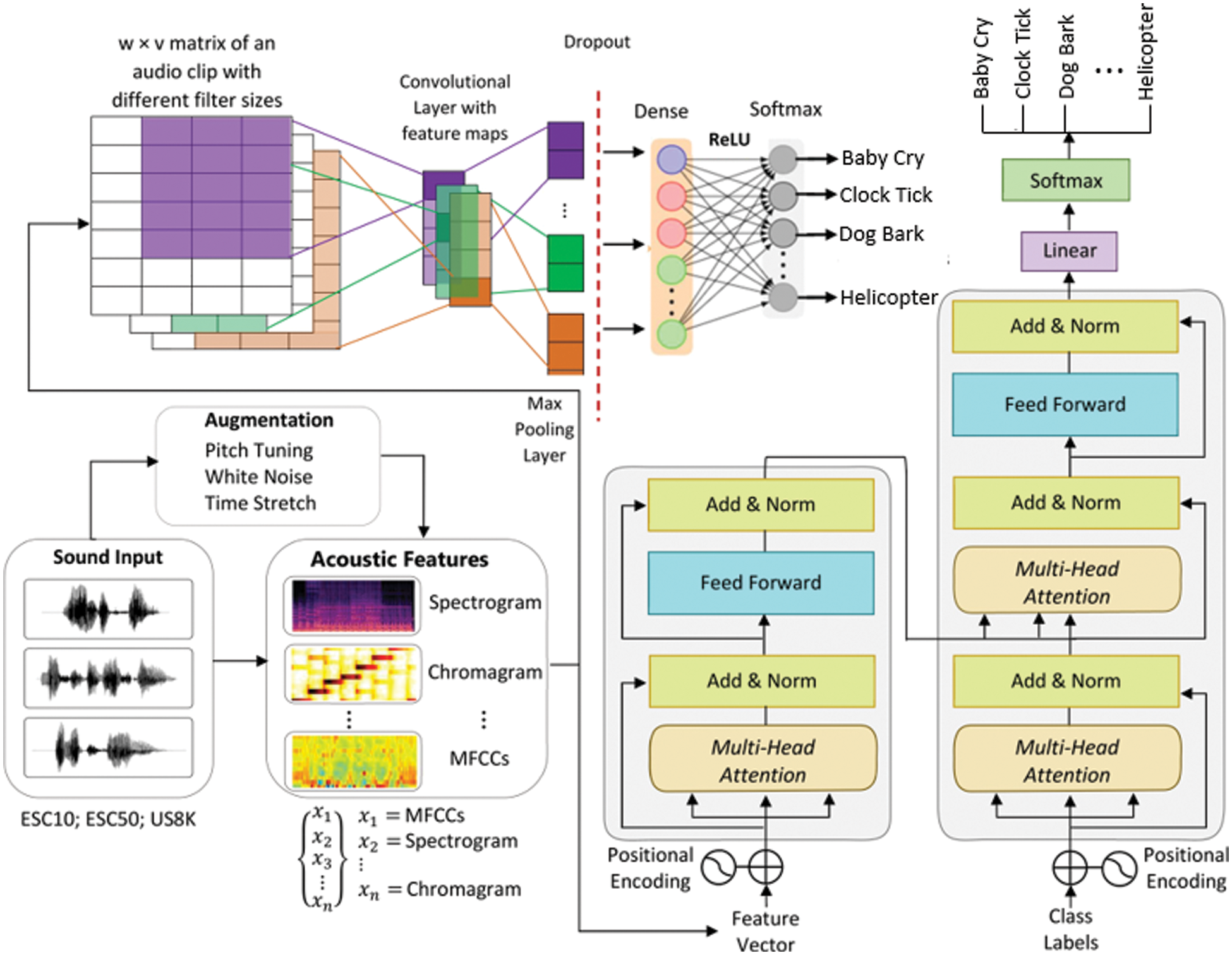
Figure 1: Proposed research methodology for ESC

3.1 Databases

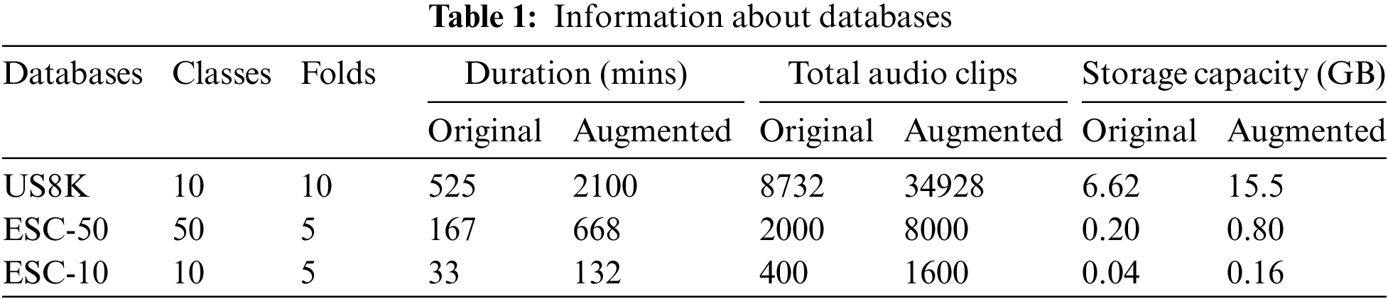
Three ESC databases were used to evaluate the classification performance of the proposed method. Three publicly available ESC databases were used to train the model and to evaluate the performance of the proposed technique, including UrbanSound8K [5], ESC-10 and ESC-50 [6]. The detailed information of these databases is presented in Tab. 1. The UrbanSound8K database contains 8732 short audio files (up to 4 s) of urban sound areas. The database is categorised into 10 classes: car horn, air conditioner, children playing, drilling, dog bark, gun shot, engine, idling, siren, jackhammer, and street music. The audio files of these classes are arranged into 10 folds. The ESC-10 database contains 400 audio files with an average time of 5 s each. These audio files involve 10 classes (rain, dog bark, baby cry, sea waves, clock tick, helicopter, person, sneeze, rooster, chainsaw, and fire crackling) with an overall duration of 33 min. This databased is dispersed into 5-folds where each fold contains 80 audio files with random distribution of sound classes. The ESC-50 database comprises 2000 short audio files which are distributed into 50 class labels in 5 major sets, including water sounds and natural soundscapes, animals, human nonspeech sounds, urban/exterior noise, and domestic/interior sounds. This database is also divided into 5-folds with 400 audio files in each fold. All audio files in ESC-10 and ESC-50 were recorded with 44.1 KHz sampling frequency, and the length of each file is 5 s.

3.2 Data Enhancement

One of the widely applied methods in environmental sound classification to avoid overfitting machine learning models is data enhancement [21]. Data enhancement is the process of increasing the size of training data using methods such as adding Gaussian noise, pitch shift, and time stretch. The essence of data enhancement is to improve the robustness of the deep learning model, enhance generalization and overall accuracy, and data distribution with reduce data variance. Deep learning models requires a large amount of training data, however, collecting environmental sound data is tasking and time consuming. In this paper, we apply the above-mentioned data enhancement methods to enhance the proposed convolutional neural network model performance. First, we increased the size of the training data by adding Gaussian noise. One of the major factors to consider when increasing the training data using Gaussian noise is the value of noise amplitude (“σ”). It is essential to choose the right value of σ. When the value of a is too large, optimization of the model would be difficult and might lead to low performance, while a small value of may weaken the performance of the model. Second, we generate new sounds by applying pitch shift enhancement which helps to shift the signal pitch wavelength by a series of n steps. The shift in the signal does not affect its duration. Finally, the tempo and pitch of the signal altered using a time stretching approach. These methods provide a means to increase the training data and avoid overfitting our proposed CNN model.

3.3 Feature Extraction

Feature extraction process plays a significant role in environmental sound classification. It helps to reduce computational time, classification errors, and algorithm complexity. Therefore, the process is essential for extraction of the most discriminant attributes from the audio signals that best describe the sound of the environment. In this paper, various features were extracted and trained with the proposed convolutional neural networks. The features extracted from ESC-10 and ESC-50 [6] and UrbanSound8K [5] datasets include Mel-spectrogram, Chromagram, MFFCs, delta MFCCs, delta-delta MFCCs and Tonnetz representation and Spectral Contrast.

•   Mel-spectrogram features: Mel-spectrogram features were extracted by dividing the audio signal into frames and computing the Fast Fourier transform of each obtained frame. The Mel-scale for the speech signal frame is produced by separating the frequency spectrum into a frequency of equal space.

•   Chromagram features: Chromagram features are used to distinguish the representation of harmony and pitch classes. To obtain chroma features, we extracted 12 distinct pitch classes from the audio signal through binning method and STFF.

•   MFFCs, delta MFCCs, delta–delta MFFCCs based features: MFCC features are a set of Mel-frequency Cepstrum that represents the short-term power spectrum of an audio signal. Cepstrum is used to determine the exact response of the human ear and allow for better audio classification due to its equally spaced frequency band. In this study, we extracted three mel-cepstrum features which include 40 sets of MFCC, delta MFCC, and delta–delta MFCC features. To extract MFCC features, the first an audio file is divided into definite length frames. In the second step, a windowing operation is performed to minimize the silence at the start and end of every frame. Afterwards, the Fast Fourier Transform (FFT) of each frame is taken to convert the time domain signal into the frequency domain. All frequency values computed from FFT are measured by using the Mean scale filter bank using Eq. (1):

Mel(f)=2595×log10(1+f700)(1)

Then, the logs of the powers are computed at each mel frequency and finally all log-Mel spectrums are transformed back to time domain using Discrete Cosine Transform (DCT). The amplitudes derived from the resultant spectrum are called the MFCCs.

•   Tonnetz based features: This is the six-dimension pitch space that describes the harmonic network of pitch relations in the fall and rise of speech signals. Features such as tonal (pitch space) of all frames of the audio signals are important in distinguishing environmental sound.

•   Spectral contrast-based features: These are features obtained by computing the root mean square (RMS) difference between the spectral proof and the spectral peak of signal frames.

In this study, we extracted a total 273 features of the above features, which include 128 melspectrogram, 12 chromagram, 40 MFFC, 40 delta-MFCC, 40 delta-delta MFCC, 6 tonnetz, and 7 spectral contrasts that were combined to train the proposed transformer and convolutional neural network models.

3.4 Proposed CNN Model

The proposed CNN model consists of five 1D convolutional layers (Conv1D), each convolutional layer is followed by plenty of other layers including among these are batch normalization layer, MaxPooling layer, dropout layer, flattened layer, and dense layer. The convolution layer used in our methodology acts on the kernels and sound data array. The first convolution layer is fed with the extracted feature matrix as input to generate the structural or detailed semantic feature map (local features) from the provided input sound files. The input of the first Conv1D consists of an array list of size 273 × 1 along with a stride of one pixel while the number of filters is 64 and with a kernel size of 5. A batch normalization layer follows this first convolution layer; this will standardize the inputs by transforming the negative values to zero and to help to attain nonlinearity in the model. Batch normalization will help to mitigate the effect of unstable input values with the help of scaling and shifting operation. A 20% dropout rate is applied afterwards during the training process. The dropout layer helps to reduce the overfitting issue by removing the input values that are less than the dropout rate. The next layer after the dropout layer is the maxpooling layer, we have used a one-dimensional maxpooling layer which consists of a pooling window of size 4. The MaxPooling layer help to reduce the feature by applying maximum filter activation at different positions of the quantified windows to produce a single output feature map.

Next, the second and third iteration convolution layer follows the similar layout of all layers described for the first convolution layer. However, the number of filters applied for these two iterations are 128 with the kernel size of 5. While for the fourth and fifth convolution layers consists of 256 filters with having the same stride and kernel size. After these sets of convolution layers, flatten, a layer is added to flatten the input sound data to one-dimensional array. A fully connected dense layer is used at the next in our proposed CNN model. The number of neurons in this layer can vary between 10 to 50 neurons; the number of neurons is subject to the number of classes we have used. The fully connected dense layer integrates the global features derived from the previous layers; it also generates a feature vector for the classification.

For the activations we have used SoftMax layer which performs the output as multilabeled classification. This also depends on the number of classifications used for environmental sound data; other parameters include an Adam optimizer having a learning rate of 0.0001, batch size of 16, and 100 epochs. Some operations and techniques used for our proposed CNN model that are worth mentioning here include activation function, dropout, and SoftMax function. The activation function is an important component of neural networks that transforms the signals of neurons to normalize output. We have used Rectifier Linear Unit (ReLU) activation function instead of sigmoid activation function to accelerate the convergence and to sort out the problem of vanishing gradient. It also helps to clamp down negative values from the neuron to 0 and positive value remain unaffected. The results of this transformation are utilized as the output of the current layer and as inputs to the consecutive layer in our proposed CNN model. The dropout technique helps to reduce the number of interconnections among the neurons in the CNN. Random process is followed, hence at every training step each neuron could be dropped out from the collated contributions of the connected neurons. We have also used SoftMax activation function as the last activation function to normalize output of the proposed CNN. The output of SoftMax function is a vector with probabilities of each possible outcome from the classifications used for environmental sound data.

3.5 Transformer Model

The vanishing gradient is the common issue in Recurrent Neural Network (RNN) and Long Short-Term Memory (LSTM) architectures regarding learning longer sequences. Although, the problem of RNN was resolved by LSTM by using carry-forward method, that carry-forward has information of the previous hidden layer and pervious of the previous hidden layer and so on. However, this carrying forward method in LSTM may fail when it comes to long sequential problem. Therefore, the transformer having self-attention mechanism is used to compute the representations of input and output without utilizing the aligned convolution or RNNs. Self-attention mechanism relates to the various positions of one sequence to compute the representation of that sequence. The structure of transformer model is stack-based having encoder-decoder components along with the self-attention.

Encoder: The encoder is used to map the input sequence to sequence of continuous representation. At every step, the transformer model consumes the previously generated representation as addition input sequence when generate the next. In this paper, the encoder was comprised of a stack of 6 similar layers where each layer was further comprised of two sub-layers namely multi-head self-attention layer and fully connected feed-forward network. Around every two sub-layers, a residual connection was employed, followed by the normalisation layer.

Decoder: The decoder was also comprised of a stack of 6 similar layers. Additionally, a third sub-layer called masked multi-headed attention was inserted in the decoder to ensure the predication of any sequence is only based on tokens before the current token. Finally, like encoder, residual connections were employed around all sub-layers, followed by the normalisation layer.

Attention: It enables the model to focus on other audio sequences in the input that are closely related to that word. Self-attention mechanism is being capable of maintaining the context-based information in an audio sequence. This information is being extracted from a set of Quires Q, keys K, and values as shown in Eq. (2):

Attention(Q,K,V)=Softmax(QKT)V(2)

The output of a given equation is a matrix that holds the information of each sequence of audio. Transformers can achieve parallelization during training because one the reason is that these Q, KV are in the stacked as matrix.

Moreover, all the encoder and decoder layers had a fully connected feed-forward network that was applied to every position individually and identically. This comprise of two linear transformations separated by a ReLU activation. In addition, learned embeddings were employed to transform the input and output tokens to dimensional vectors. Finally, a softmax function was used to transform the decoder output to compute the class probabilities.

3.6 Evaluation Metrics

The performance of each ESC model was evaluated using different evaluation metrics. These evaluation metrics include accuracy, F1-score, precision, and recall. For each sound class, the detection was measured with the labels and the number of false-positive (FP), true positive (TP), false-negative (FN), and true negative (TN) were computed using the confusion matrix of each prediction. Accuracy computes the frequency of accurately detected respiratory sound classes from the total number of sound signals by using Eq. (3).

Accuracy=1N∑i=1N(TP+TN)i(TP+TN+FP+FN)i(3)

where N shows the number of sound files.

A recall is used to calculate the number of accurately detected instances as positive instances using Eq. (4) while precision is used to evaluate the performance of the proposed models to correctly detect actual sound file as given in Eq. (5).

Recall=1N∑i=1N(TP)i(TP+FN)i(4)

Precision=1N∑i=1N(TP)i(TP+FP)i(5)

In addition, these evaluation metrics have been widely employed for the evaluation of various disease detection, classification, and related systems [22,23].

3.7 Experimental Setup

We conducted all experiments using the anaconda, open-source software library that is used in Python programming. It has various inbuilt machine learning algorithms and data science packages, including NumPy, pandas, scikit-learn, etc. It also has some statistical packages for insight visualization such as matplotlib, seaborn. It can function effectively in Windows and Linux operating system platforms. It also offers a choice of creating various environments to perform various tasks using specific packages.

To implement the transformer and CNN models from scratch, Keras library has been utilized. It provides easiness to users to add or drop layers, max-pooling functions, and activation functions in both transformer and CNN. Another important python library known as Librosa is utilized to conduct experiments for ESC. The purpose of this library is the evaluation of sound signals. In this study, the seven acoustic feature extraction techniques used can be obtained using this package. These feature extraction techniques are MFCC and its variants (delta, delta–delta), Mel spectrogram (Mel), Chromagram, Tonnetz, and Spectral Contrast. This library executes the data enhancement techniques involved in this study. Moreover, the experiments reported in this study were conducted on a laptop of Apple MacBook Pro. The processor of the system is 2.5 GHz Dual-Core Intel(R) Core i5 with a memory of 8 GB. The hard drive includes 512 GB SSD + 512 GB external HDD.

4  Results and Discussion

In this section, we present the performance evaluation of transformer and CNN models on the original ESC-10, ESC-50, and UrbanSound8K datasets and enhanced datasets. The pre-divided 10 fold cross validation data split method was employed in all experiments, which implies that each data sample was used in both training and test databases.

4.1 Results on the ESC-10 Database

The Tab. 2 and Fig. 3 illustrates the performance of CNN and transformer models by using the Mel-spectrogram, Chromagram, MFFCs, delta MFCCs, delta-delta MFCCs, Tonnetz representation and Spectral Contrast feature extraction methods on the original ESC-10. As shown in the table, we have achieved the weighted test accuracy of 0.85 by using CNN model and 0.86 by using the transformer model. In addition to this, we have evaluated the results on the basis of precision, recall, and F1-score. We have observed the highest F1-score of 1.00 in Baby cry class by using CNN model and the lowest 0.67 in the rain class. For the rest of the class F1-score was in between 0.71 to 0.94. The highest recall score was achieved 1.00 in Helicopter, Rooster, and Fire classes and the rest classes were in between 0.67 to 0.92. Similarly, for precision, the highest score was obtained by 1.00 in Chainsaw class. Besides this, we evaluated the transformer model on the ESC-10 dataset and observed that the transformer model performed better than CNN model in terms of accuracy and training time as shown in Tab. 8. Moreover, the Fig. 2 demonstrate the training vs. validation accuracy of transformer and CNN models on the original and enhanced ESC-10 dataset.

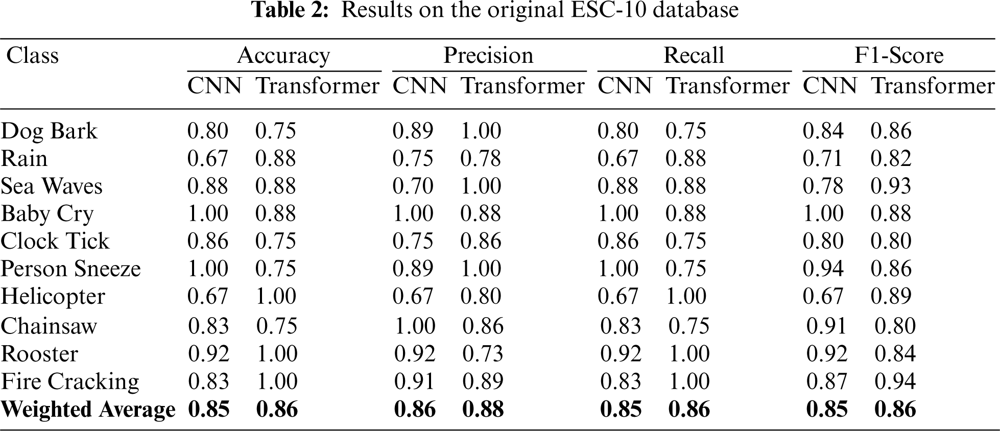
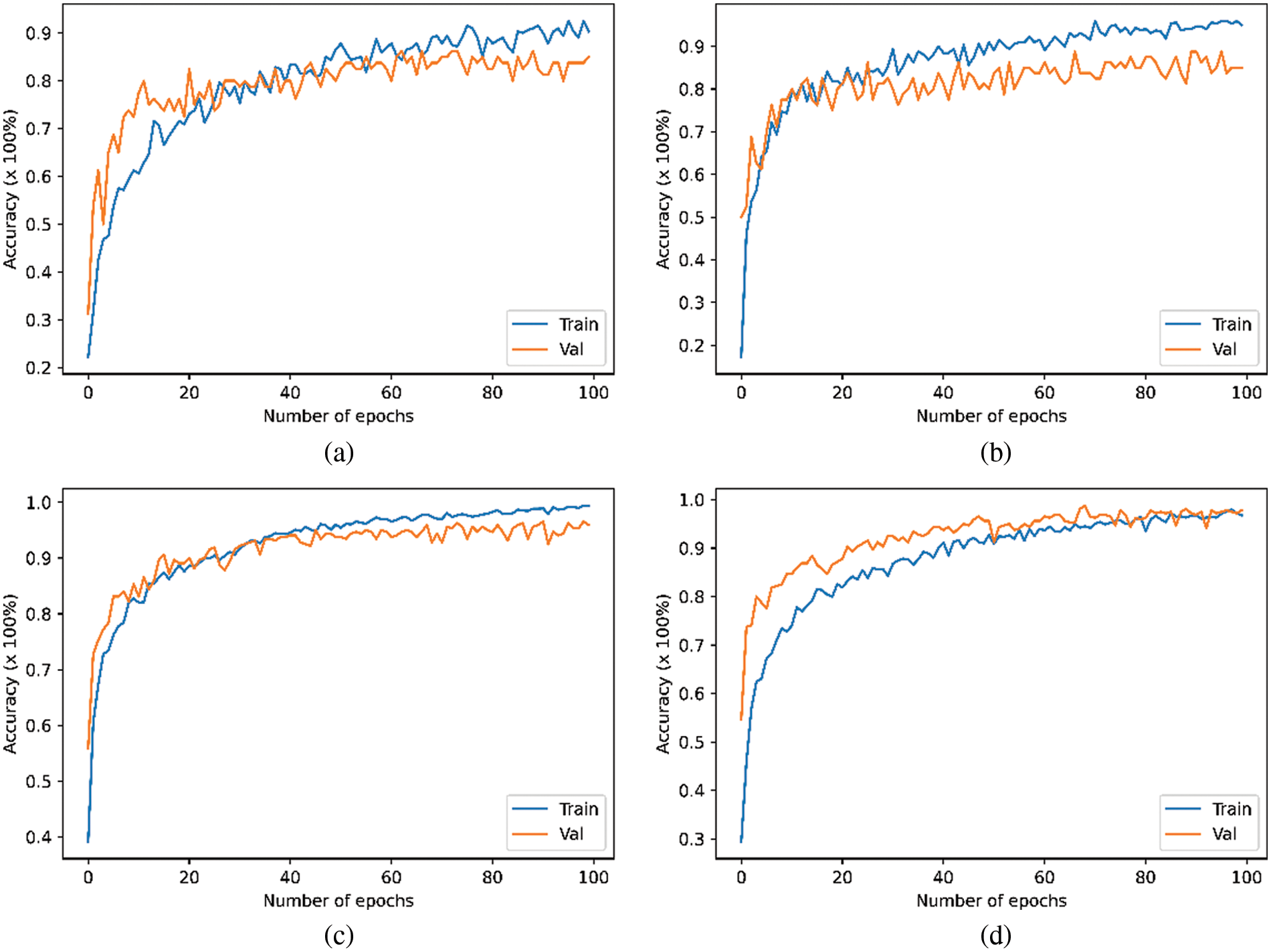
Figure 2: Performance on ESC-10 (a) CNN performance on the original data (b) Transformer performance on the original data (c) CNN performance on the enhanced data (d) Transformer performance on the enhanced data

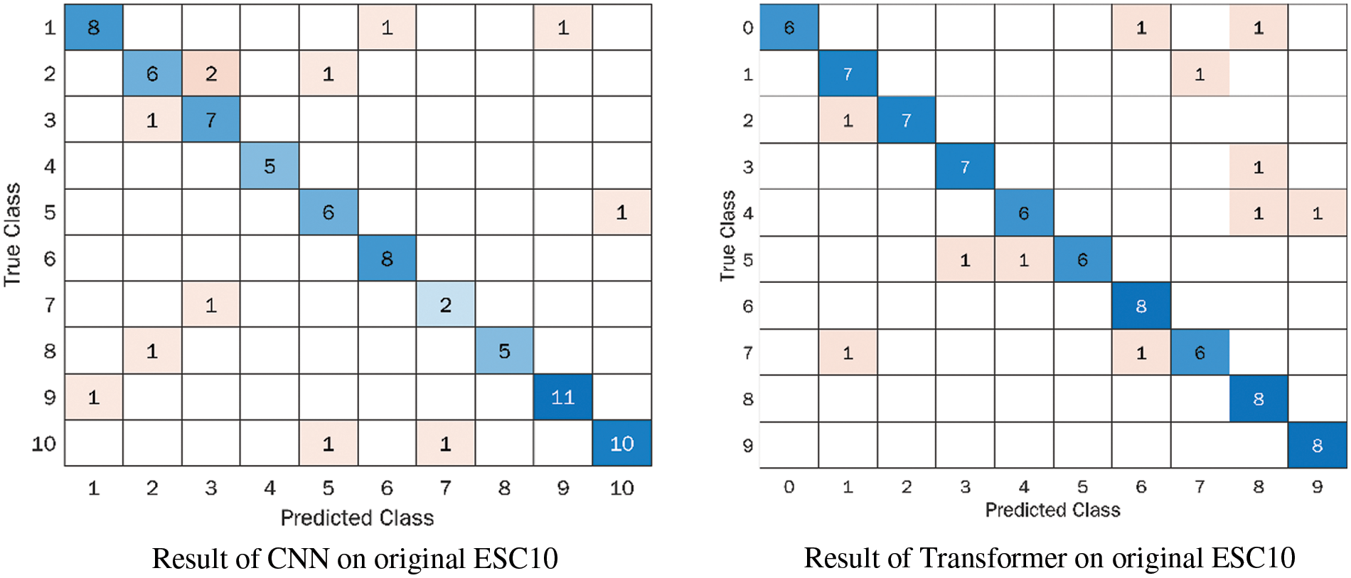
Figure 3: Confusion metrics for the original ESC-10 database

To avoid the risk of overfitting problem, the data enhancement methods were applied to the audio files. After the data enhancement, both CNN and transformer models receive enough training data as input. The experimental results demonstrated in Tabs. 3 and 8 reveals the benefit of employing data enhancement for training both CNN and transformer models. The difference between the average accuracies achieved by both models on the original and the enhanced datasets is around 11%. The transformer model obtained the highest accuracy of 0.97 with the enhanced ESC-10. The accuracy of each class is presented in Fig. 4.

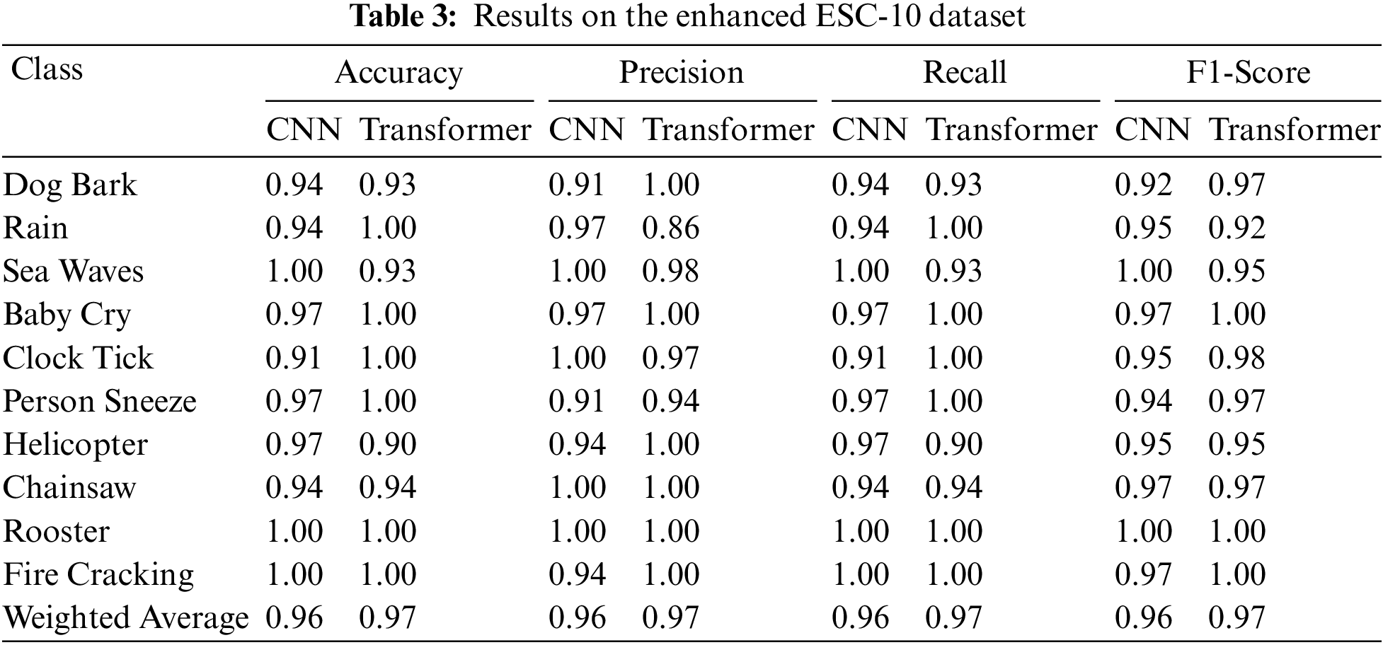
Figure 4: Confusion metrics for the original ESC-10 database with enchantment

4.2 Results on the ESC-50 Database

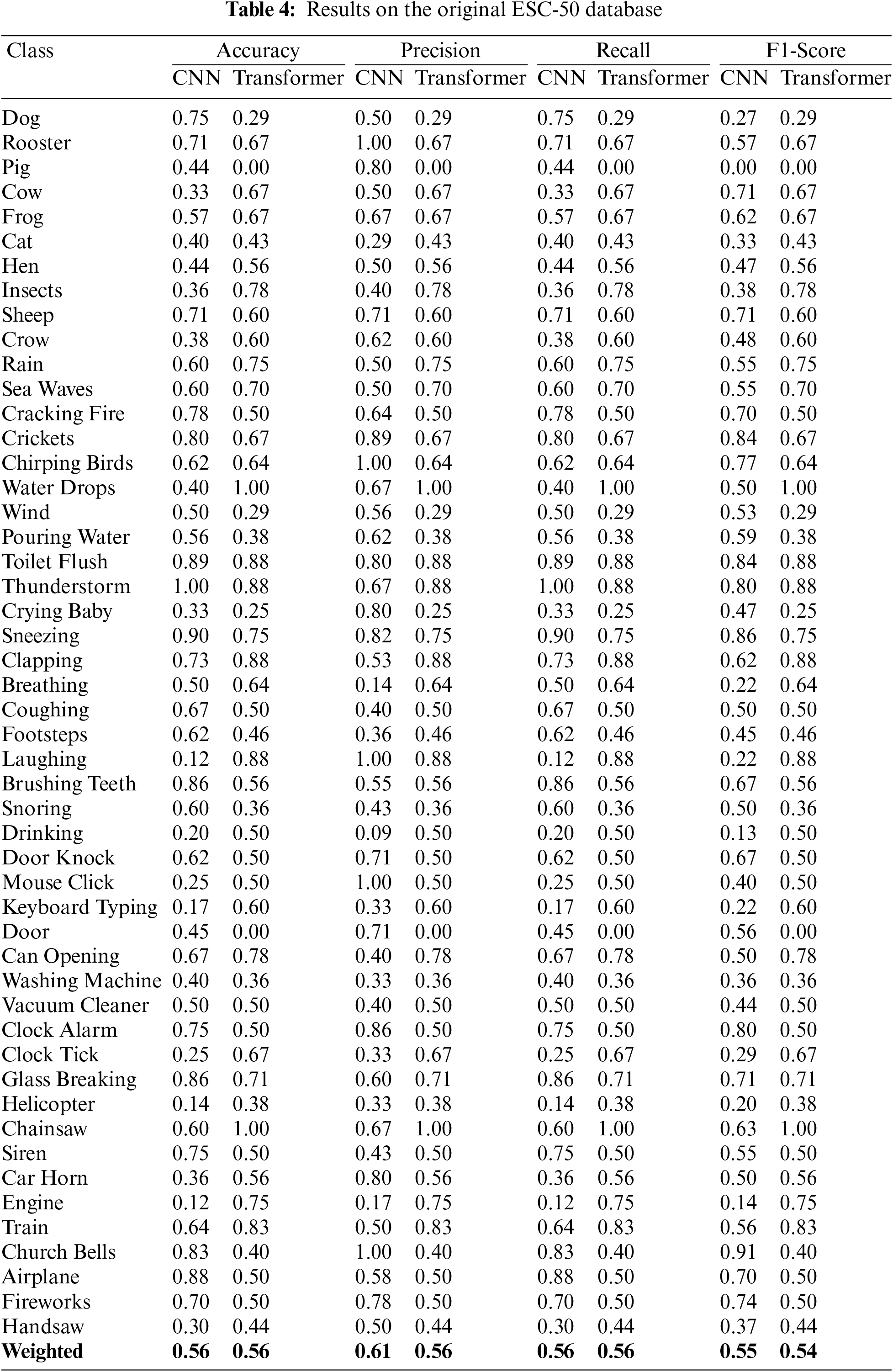
The ESC-50 database is substantially more complicated and comprehensive. The possibility of overfitting issue is higher than ESC-10 database because ESC-50 contains a larger number of classes and a small number of audio files for model training. Tab. 4 demonstrate the performance of CNN and transformer models on the original ESC-50 database. The experimental results again exhibit the advantages of using transformer as it requires less training time compared to CNN and the best accuracy of 0.57 was achieved as shown in Tab. 8.

Subsequently, the results shown in Tab. 4 illustrate that ESC-50 is the highly affected dataset compared to ESC-10 because of the overfitting issue. To overcome the issue of overfitting, three data enhancement methods were applied on ESC-50 dataset. The experimental results as presented in Tab. 5 demonstrate the improvement related to the overfitting issues. The highest achieved accuracy was 0.94 by again transformer model and outperformed the CNN in both accuracy and training time. Moreover, the training vs. validation accuracy of transformer and CNN models on the original and enhanced ESC-50 dataset is illustrated in Fig. 5.

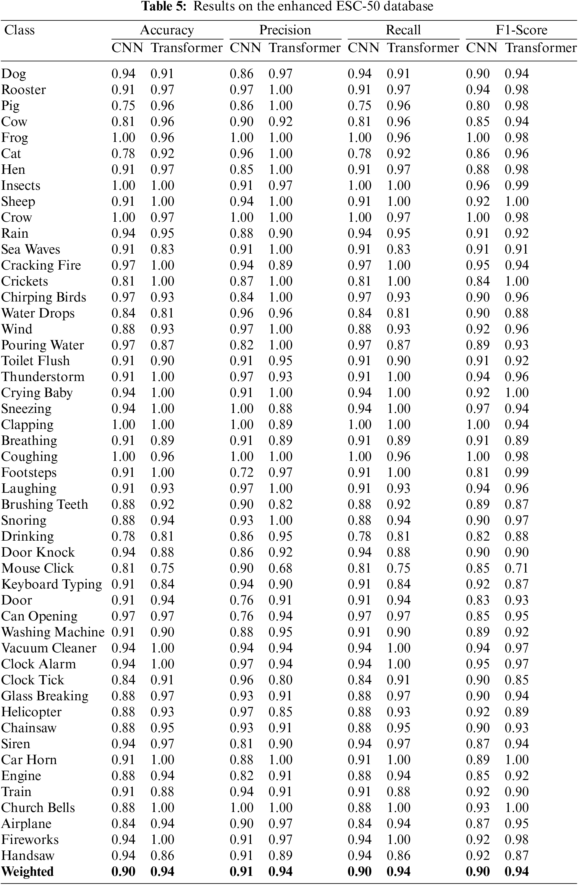
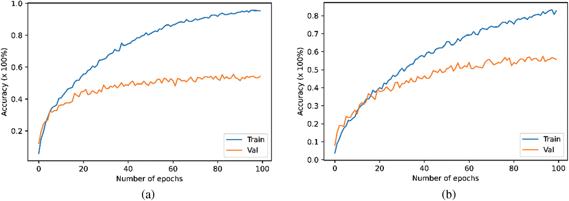
Figure 5: Performance on ESC-50 (a) CNN performance on the original data (b) Transformer performance on the original data (c) CNN performance on the enhanced data (d) Transformer performance on the enhanced data

4.3 Results on the Urbansound8k Database

The overfitting issue may be insignificant in this database due to its size. The UrbanSound8K database contains a smaller number of classes (10) and a large number of audio files (8732) for the training of CNN and transformer models. Tab. 6 illustrates the performance of both models on the original UrbanSound8K database. Again, the highest accuracy was 0.94 by the transformer model combined with seven acoustic features (mel spectrogram, chromagram, MFFCs, delta delta MFCCs, delta-delta MFCCs, Tonnetz representation and spectral contrast). The classification accuracy of each class in this database for both CNN and transformer models is presented in Figs. 6a and 6b respectively.

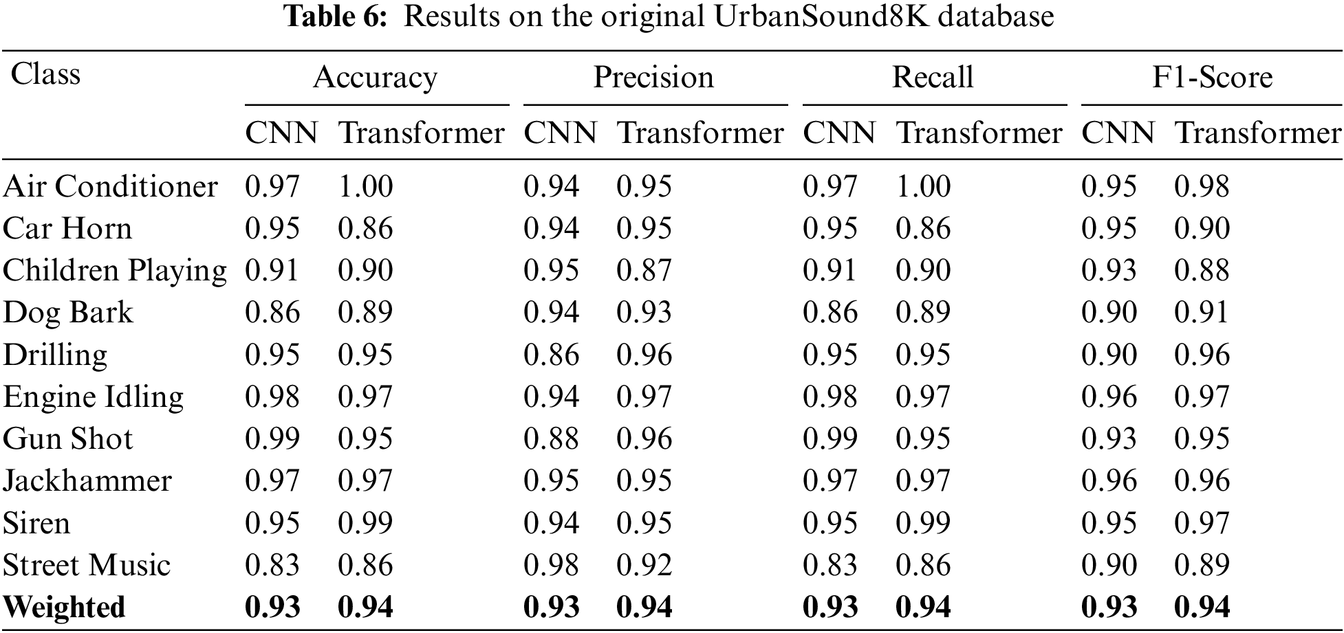
Figure 6: Confusion metric on original US8k

Tab. 7 demonstrates the experimental results of CNN and transformer models on the enhanced UrbanSound8K database. The best achieved accuracy was 0.98 exhibited by both models. However, the transformer model performed better than CNN as it consumed less time for training as shown in Tab. 8. The accuracy difference between the enhanced and original UrbanSound8K database is minimal as the original UrbanSound8K database already contains large amount of audio files. The classification accuracy of each class in this database for both CNN and transformer models is presented in Figs. 7a and 7b respectively. In addition, the Fig. 8 shows the training vs. validation accuracy of transformer and CNN models on the original and enhanced UrbanSound8K dataset. Finally, the Tab. 8 summarizes the results of the detailed comparison and analysis and of all databases.

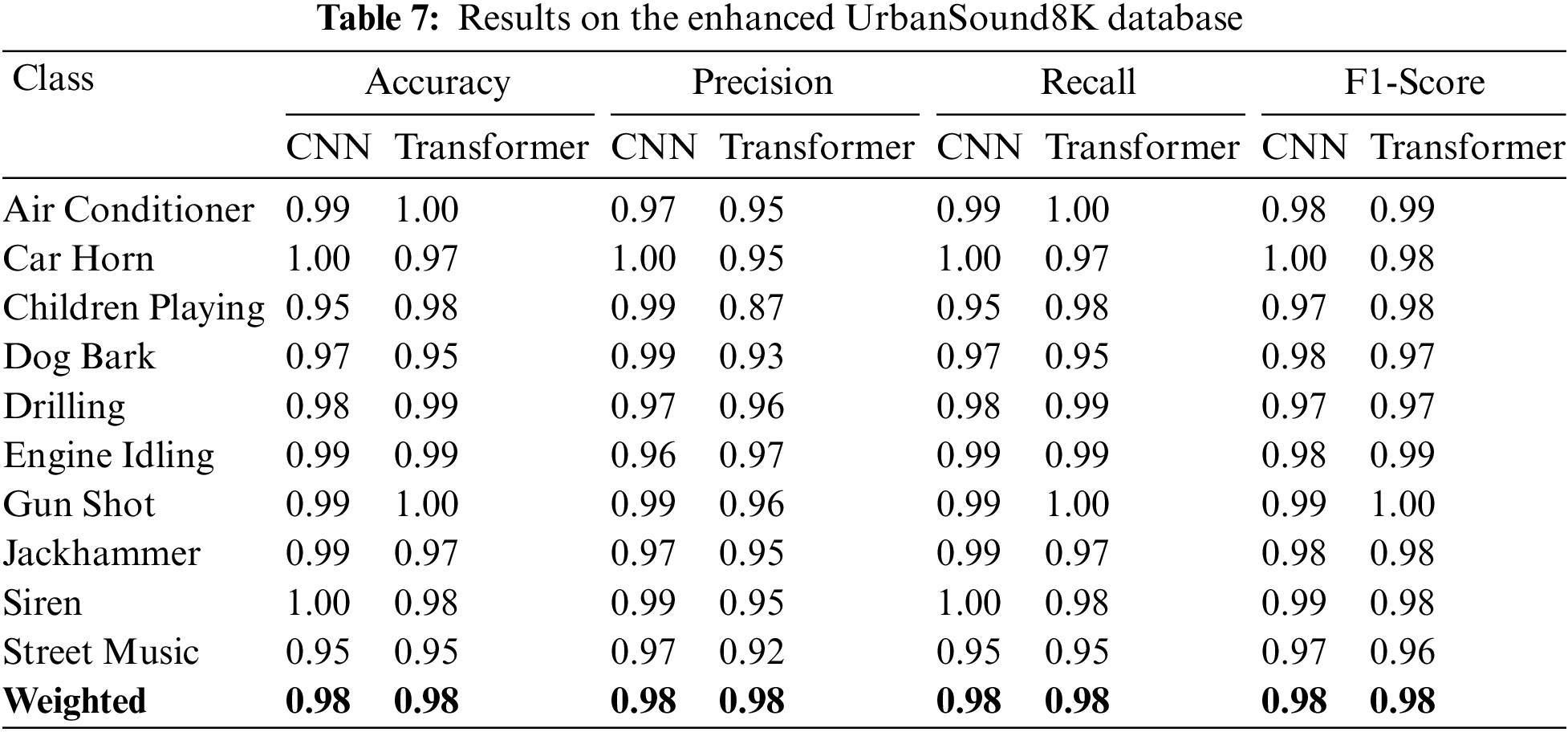
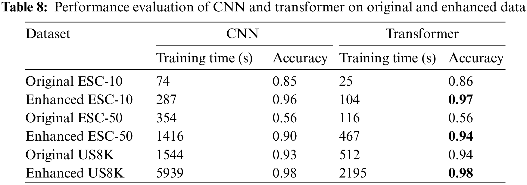
Figure 7: Confusion metric using the enhanced UrbanSound8K database with data enhancement

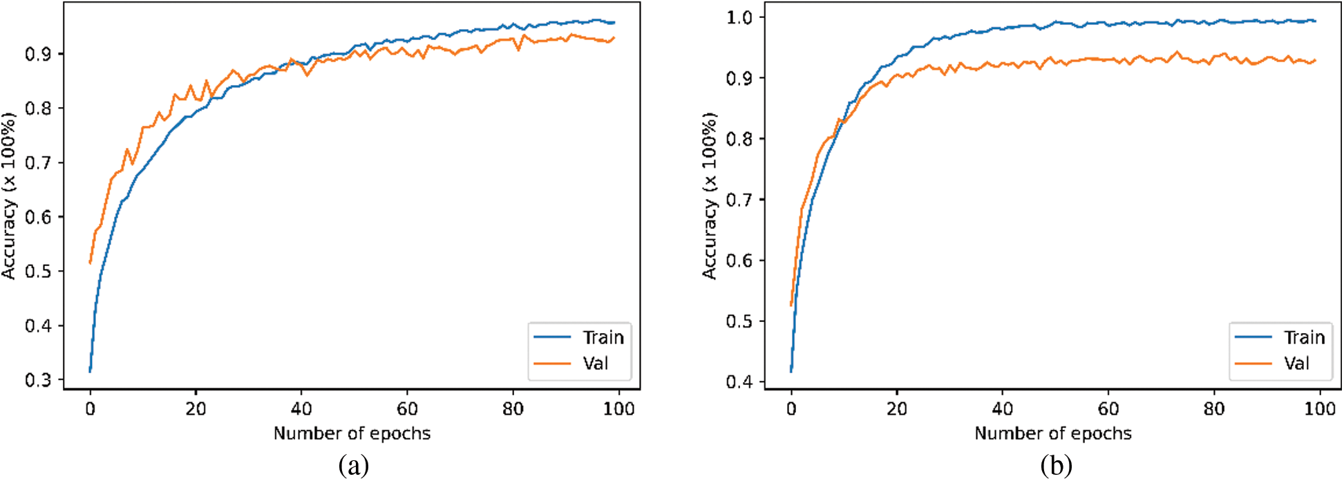
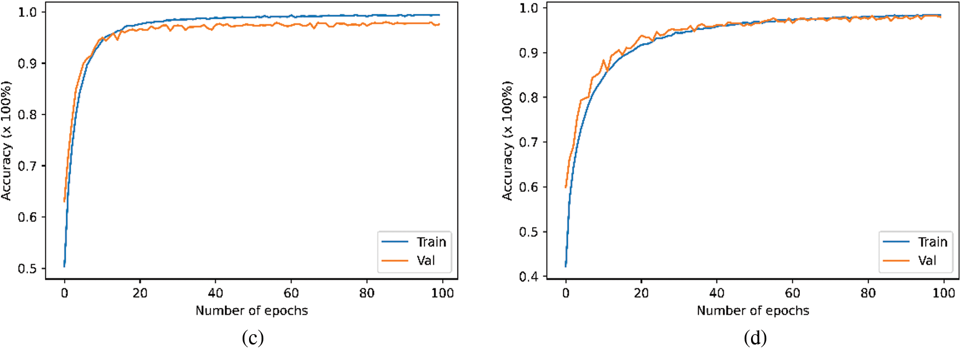
Figure 8: Performance on US8K (a) CNN performance on the original data (b) Transformer performance on the original data (c) CNN performance on the enhanced data (d) Transformer performance on the enhanced data

4.4 Comparison with Existing Methods on ESC

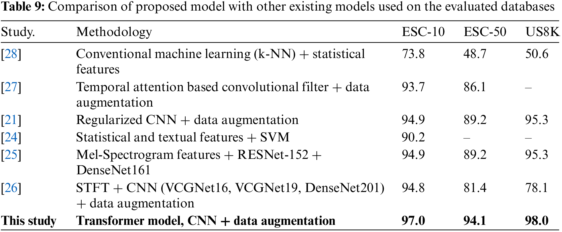
To investigate the significance of the proposed environmental sound classification using transformer based deep learning methods, we compared the proposed transformer model with existing studies in environmental sound classification using similar datasets. Six (6) recent studies on environmental sound classification were chosen. These include [21,24–28]. In [24] proposed hybrid feature generation method to extract statistical and textual features from sound wave for ESC. Here, the feature vectors extracted were categorized into one-dimensional local binary feature pattern (1D-LBP), one-dimensional ternary feature (1D-TP), and statistical features such as mean, median etc. The extracted features were fed to a 3rd polynomial order kernel-based support vector machine and achieved a classification accuracy of 90.2%. Reference [25] proposed convolutional neural network with data enhancement to automatically extract Mel-Spectrogram features from an audio clip. In addition, the study used CNN model learned from scratch transfer learning mechanism and data enhancement although signal variation applied to the audio clips. The study achieved 94.9%, 89.2%, and 95.3% accuracy on ESC-10, ESC-50, and US8K datasets, respectively. In a similar study [26], authors evaluated the impact of deep convolutional neural networks and denoised sound wave using STFT for ESC. The authors deployed pretrained CNN models such as VCGNet16, VCGNet19, and DenseNet201 for automatic feature extraction. Then the extracted feature sets were fed to the support vector machine for ESC. Furthermore, authors [21] proposed regularized deep convolutional neural networks for ESC. The study extracted features such as MFCC, Mel-Spectrogram, and Log-Mel from the sound wave. To avoid overfitting the CNN model and improve the performance results, the authors applied data enhancement techniques such as shifting, adding white noise, and positive pitch to increase the size of the data.

Other studies having similar implementation approaches to the current studies are the ones proposed by [27,28]. While [27] introduced temporal attention based deep convolutional neural networks for ESC, [28] proposed implementation of urban sound classification on-board embedded systems. The proposed implementation was evaluated using conventional machine learning models. The performance results obtained by these studies using ESC-10, ESC-50, US8K dataset, and different machine learning models are presented in Tab. 9. The result obtained by our proposed transformer model and data enhancement is shown in the last row of Tab. 9. From the table, it is clear that the proposed model clearly outperformed other baseline studies for ESC. The high performance of the proposed transformer model is as a result of its ability to utilize the data enhancement to automatically extract the relevant features from the sound waves. Hence, the performance of the transformer model was improved on all used databases as compared to other baseline studies presented in Tab. 9.

5  Conclusion

ESC is a challenging problem because of the extraction of relevant features and classification. In this paper, 1D CNN and transformer models for ESC were evaluated on the original and enhanced data using seven different features. The performances of the proposed CNN and transformer models were examined using the ESC-10, ESC-50, and UrbanSound8K datasets to demonstrate the robustness and significance. The reported results showed that the proposed transformer model coupled with seven features using all three datasets outperforming the baseline models. The transformer model achieved 97.0% accuracy for the ESC-10 enhanced dataset, 94.1% for the ESC-50 enhanced dataset, and 98.0% for the UrbanSound8K enhanced dataset. In addition, the proposed transformer model achieved 86%, 56%, and 94% accuracy on ESC-10, ESC-50, and UrbanSound8K dataset, respectively, without using data enhancement techniques. This article shows that the proposed transformer model can achieve the best accuracy for the ESC task. The future work may be on the study of the selection of optimal features and the evaluation of other deep learning models to obtain high-level features. Because of the size constraints and computational complexity, in future the environmental sound classification (ESC) models will be trained and deployed on the cloud. To use these cloud-based trained deep learning models in real time, mobile applications will transfer input voice over the network.

Funding Statement: The authors are grateful to the Taif University Researchers Supporting Project number (TURSP-2020/36), Taif University, Taif, Saudi Arabia.

Conflicts of Interest: The authors declare that they have no conflicts of interest to report regarding the present study.

References

 1.  S. Chu, S. Narayanan and C. -C. J. Kuo, “Environmental sound recognition with time-frequency audio features,” IEEE Transactions on Audio, Speech, and Language Processing, vol. 17, no. 6, pp. 1142–1158, 2009. [Google Scholar]

 2.  P. Foggia, N. Petkov, A. Saggese, N. Strisciuglio and M. Vento, “Reliable detection of audio events in highly noisy environments,” Pattern Recognition Letters, vol. 65, pp. 22–28, 2015. [Google Scholar]

 3.  R. Jahangir, Y. W. Teh, G. Mujtaba, R. Alroobaea, Z. H. Shaikh et al., “Convolutional neural network-based cross-corpus speech emotion recognition with data augmentation and features fusion,” Machine Vision and Applications, vol. 33, no. 3, pp. 1–16, 2022. [Google Scholar]

 4.  R. Jahangir, Y. W. Teh, N. A. Memon, G. Mujtaba, M. Zareei et al., “Text-independent speaker identification through feature fusion and deep neural network,” IEEE Access, vol. 8, pp. 32187–32202, 2020. [Google Scholar]

 5.  J. Salamon, C. Jacoby and J. P. Bello, “A dataset and taxonomy for urban sound research,” in Proc. of the 22nd ACM Int. Conf. on Multimedia, Lisboa, Portugal, pp. 1041–1044, 2014. [Google Scholar]

 6.  K. J. Piczak, “ESC: Dataset for environmental sound classification,” in Proc. of the 23rd ACM Int. Conf. on Multimedia, Lisboa, Portugal, pp. 1015–1018, 2015. [Google Scholar]

 7.  X. Valero and F. Alias, “Gammatone cepstral coefficients: Biologically inspired features for non-speech audio classification,” IEEE Transactions on Multimedia, vol. 14, no. 6, pp. 1684–1689, 2012. [Google Scholar]

 8.  K. J. Piczak, “Environmental sound classification with convolutional neural networks,” in 25th Int. Workshop on Machine Learning for Signal Processing (MLSP), Boston, USA, pp. 1–6, 2015. [Google Scholar]

 9.  I. McLoughlin, H. Zhang, Z. Xie, Y. Song and W. Xiao, “Robust sound event classification using deep neural networks,” IEEE/ACM Transactions on Audio, Speech, and Language Processing, vol. 23, no. 3, pp. 540–552, 2015. [Google Scholar]

10. T. H. Vu and J. -C. Wang, “Acoustic scene and event recognition using recurrent neural networks,” in Proc. of Detection and Classification of Acoustic Scenes and Events, Budapest, Hungary, pp. 1–3, 2016. [Google Scholar]

11. A. Guzhov, F. Raue, J. Hees and A. Dengel, “Esresnet: Environmental sound classification based on visual domain models,” in 25th Int. Conf. on Pattern Recognition (ICPR), Milan, Italy, pp. 4933–4940, 2021. [Google Scholar]

12. Y. Tokozume, Y. Ushiku and T. Harada, “Learning from between-class examples for deep sound recognition,” arXiv, vol. abs/1711, pp. 10282, 2017. [Google Scholar]

13. A. Pillos, K. Alghamidi, N. Alzamel, V. Pavlov and S. Machanavajhala, “A real-time environmental sound recognition system for the Android OS,” in Proc. of Detection and Classification of Acoustic Scenes and Events, Budapest, Hungary, pp. 1–5, 2016. [Google Scholar]

14. B. Zhu, C. Wang, F. Liu, J. Lei, Z. Huang et al., “Learning environmental sounds with multi-scale convolutional neural network,” in Int. Joint Conf. on Neural Networks (IJCNN), Rio de Janeiro, Brazil, pp. 1–8, 2018. [Google Scholar]

15. Y. Tokozume and T. Harada, “Learning environmental sounds with end-to-end convolutional neural network,” in Int. Conf. on Acoustics, Speech and Signal Processing (ICASSP), New Orleans, Louisiana, USA, pp. 2721–2725, 2017. [Google Scholar]

16. D. M. Agrawal, H. B. Sailor, M. H. Soni and H. A. Patil, “Novel TEO-based Gammatone features for environmental sound classification,” in 25th European Signal Processing Conf., Kos Island, Greece, pp. 1809–1813, 2017. [Google Scholar]

17. S. Li, Y. Yao, J. Hu, G. Liu, X. Yao et al., “An ensemble stacked convolutional neural network model for environmental event sound recognition,” Applied Sciences, vol. 8, no. 7, pp. 1152, 2018. [Google Scholar]

18. M. J. A. P. A. Huzaifah, “Comparison of time-frequency representations for environmental sound classification using convolutional neural networks,” arXiv, vol. abs/1706, pp. 07156, 2017. [Google Scholar]

19. J. Salamon and J. P. J. I. S. P. I. Bello, “Deep convolutional neural networks and data augmentation for environmental sound classification,” IEEE Signal Processing Letters, vol. 24, no. 3, pp. 279–283, 2017. [Google Scholar]

20. Z. Zhang, S. Xu, S. Cao and S. Zhang, “Deep convolutional neural network with mixup for environmental sound classification,” in Chinese Conf. on Pattern Recognition and Computer Vision, Guangzhou, China, pp. 356–367, 2018. [Google Scholar]

21. Z. Mushtaq and S. -F. Su, “Environmental sound classification using a regularized deep convolutional neural network with data augmentation,” Applied Acoustics, vol. 167, no. 4, pp. 107389, 2020. [Google Scholar]

22. R. Jahangir, Y. W. Teh, F. Hanif and G. Mujtaba, “Deep learning approaches for speech emotion recognition: State of the art and research challenges,” Multimedia Tools and Applications, vol. 80, no. 16, pp. 1–66, 2021. [Google Scholar]

23. R. Jahangir, Y. W. Teh, H. F. Nweke, G. Mujtaba, M. A. Al-Garadi et al., “Speaker identification through artificial intelligence techniques: A comprehensive review and research challenges,” Expert Systems with Applications, vol. 171, no. 3, pp. 1–27, 2021. [Google Scholar]

24. E. Akbal, “An automated environmental sound classification methods based on statistical and textural feature,” Applied Acoustics, vol. 167, no. 3, pp. 1–6, 2020. [Google Scholar]

25. Z. Mushtaq, S. -F. Su and Q. -V. Tran, “Spectral images based environmental sound classification using CNN with meaningful data augmentation,” Applied Acoustics, vol. 172, no. 2, pp. 1–15, 2021. [Google Scholar]

26. F. Demir, M. Turkoglu, M. Aslan and A. Sengur, “A new pyramidal concatenated CNN approach for environmental sound classification,” Applied Acoustics, vol. 170, no. 6, pp. 1–7, 2020. [Google Scholar]

27. Z. Zhang, S. Xu, S. Zhang, T. Qiao and S. Cao, “Attention based convolutional recurrent neural network for environmental sound classification,” Neurocomputing, vol. 453, pp. 896–903, 2021. [Google Scholar]

28. B. da Silva, A. W. Happi, A. Braeken and A. Touhafi, “Evaluation of classical machine learning techniques towards urban sound recognition on embedded systems,” Applied Sciences, vol. 9, no. 18, pp. 3885, 2019. [Google Scholar]