Forecasting Future Trajectories with an Improved Transformer Network

1  Introduction

Automated driving technology has become a research hot spot due to its wide applications in intelligent transportation systems. As shown in Fig. 1, trajectory prediction [1] is essential for autonomous driving to achieve safe driving except for vehicle detection [2]. The red and orange lines represent the ego-vehicle’s future trajectory and its associations with surrounding vehicles. Studies on historical movement rules and behavior patterns of surrounding vehicles and precise prediction of their future trajectories can effectively boost driving safety and avoid vehicle collisions. For example, the ego-vehicle will not turn right to avoid a potential collision if its forward vehicle turns right in the near future.

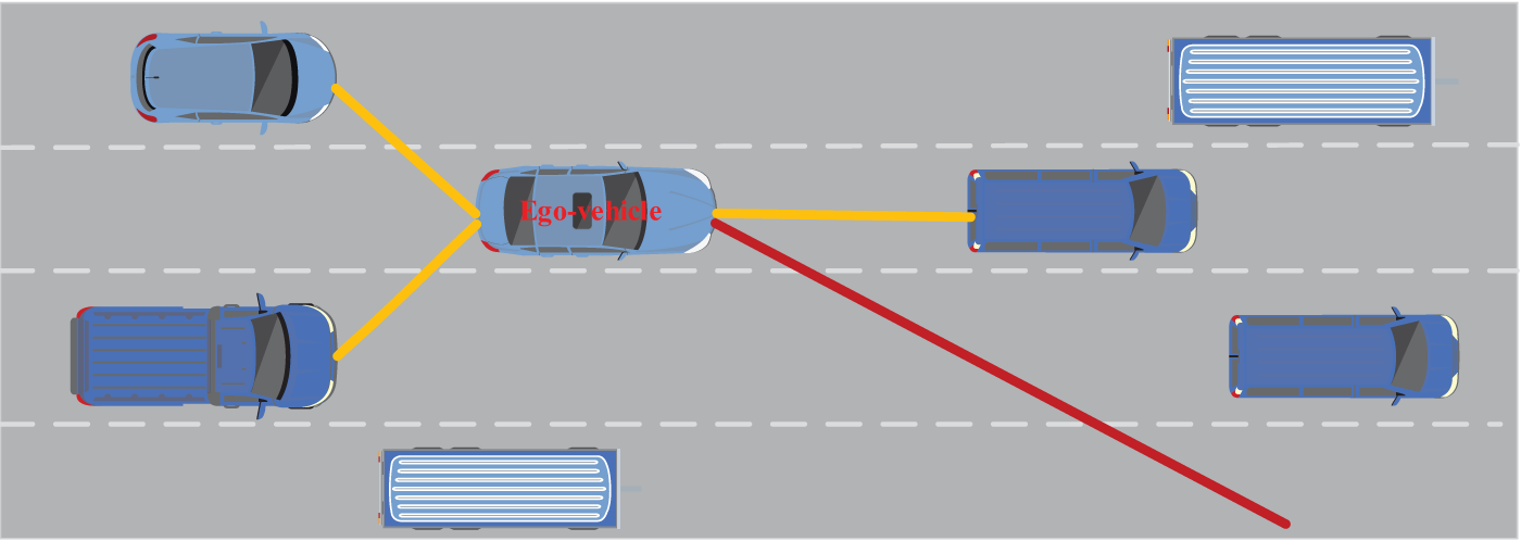
Figure 1: Driving scenario of an autonomous vehicle

With the developments of machine learning [3–5], researchers proposed two kinds of prediction methods, including model-driven [6,7] and data-driven [8–10]. For the former, some researchers used the Markov chain and Kalman filter [6,7] to perform trajectory prediction. Houenou et al. [11] proposed combining the constant yaw acceleration motion model with trajectory prediction of maneuver identification, which made up for the shortcomings of traditional prediction methods in long-term prediction. Ji et al. [12] used an encoder-decoder structure and a hybrid density network (MDN) layer for vehicle trajectory prediction. However, it is difficult for the model-driven prediction method to model the complex, realistic environment since the complexity and high non-linearity of agents’ motion.

With the rise of deep learning [13,14], many data-driven methods have been proposed in recent years since trajectory prediction could be regarded as a sequence classification or a sequence generation task. LSTM network [15] is widely used for information mining and deep representation when dealing with time-series data. Khosroshahi et al. [16] established a vehicle mobility classification framework by using the LSTM model. Phillips et al. [17] used the LSTM model to predict the trajectory direction of vehicles when they reached the intersection. Kim et al. [18] used the LSTM model to learn the time behavior of vehicles and predict future trajectories from a large number of trajectory data. Alahi et al. [19] proposed Social LSTM, which automatically learns the interaction between trajectories simultaneously by introducing the "Social" pooling layer. However, due to its cyclic structure, the LSTM model has some shortages, such as gradient explosion, sensitivity to lost data, and low prediction efficiency.

To solve the above problems, we propose to achieve trajectory prediction based on Transformer networks, which have achieved state-of-the-art performance on multiple tasks like the Natural Language Processing (NLP) [20–22]. Transformer networks utilize an attention mechanism [20], which allows the networks to focus on a different part of the input column at each time step. Hence, it could provide deeper reasoning about the correlation between input sequence data and situational interaction.

LSTM could only process sequences sequentially due to its cyclic structure, whereas Transformer networks [23,24] could process sequential input sequences in parallel through a multi-head attention mechanism and make predictions from the input with missing data. However, Transformer networks have a high space-time complexity since the self-attention mechanism is calculated as the dot product. Such a high complexity will influence the prediction efficiency of the model [25,26]. Hence, a probabilistic sparse attention mechanism is introduced to reduce attention complexity by reducing the number of query values in the attention mechanism.

To sum up, the main contributions of this paper can be summarized as follows:

1.    Considering that traditional forecasting methods do not make full use of historical information and cannot handle large amounts of data in parallel, a Transformer network is used to realize vehicle trajectory prediction in a better way.

2.    To solve the problems of attention query sparsity and the high space-time complexity in the self-attention mechanism, a probabilistic sparse self-attention mechanism is introduced to selectively calculate the query-key value and reduce the space-time overhead of the self-attention mechanism.

3.    To solve the problem that traditional activation functions are sensitive to parameter initialization, learning rate, and neuron death, activate or not (ACON) activation function [27] is utilized to determine whether the adjustment from adaptation was activated through two learnable parameters. The experimental results indicate that the proposed method could predict future trajectories precisely and efficiently.

2  Related Work

2.1 Transformer Network

Transformer networks have achieved excellent performance on multiple NLP tasks such as machine translation [28], sentiment analysis [29,30], and text generation [31]. It completely discards the recursion idea and the sequential nature of language sequence and only uses the powerful self-attention mechanism to model time series data.

As shown in Fig. 2, the Transformer network adopts an Encoder-Decoder architecture [32,33], composed of N stacked blocks. The Encoder contains the self-attention layer and the feed-forward neural network. Sequence features are extracted from the attention layer and transmitted to the decoder after processing. The decoder consists of three layers: a multi-head attention layer with a mask, a multi-head attention layer, and a feed-forward neural network. The multi-head attention layer with mask hides the output after the current time t. Hence, the prediction result of the output at the current time t does not depend on the information after t.

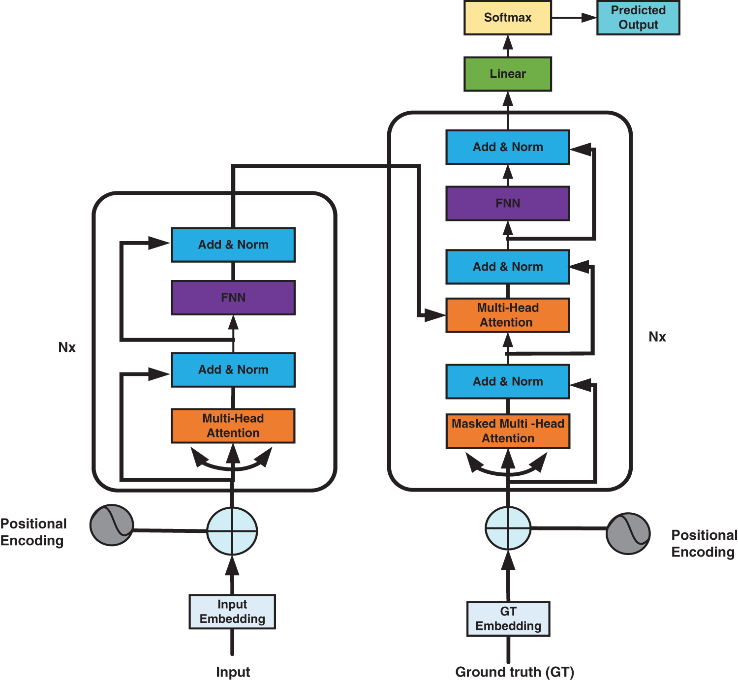
Figure 2: Structure diagram of transformer

2.2 Attention Mechanism

When the attention mechanism [34–36] generates the output at the current moment, it also generates the attention range to represent the input sequence that the output should focus on at the next moment. It allocates different weights to the sequence features, thus reducing the computing power and the limitation of the optimization algorithm and increasing the accuracy of the trajectory prediction processing. As shown in Fig. 3, the ability of the Transformer network to capture non-linearity is primarily at the self-attention level.

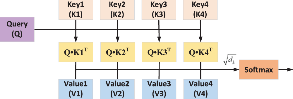
Figure 3: Structure diagram of the attention mechanism

The input consists of a Q (Query) matrix of dimension dk, a K (Key) matrix, and a corresponding V (Value) matrix of dimension dv. In each attention layer, Q and K calculate the degree of attention S between vectors through S = Q•KT, and the normalized score Sn obtained by scaling through Sn=S/dk to optimize the training effect. Then, the Softmax() function is applied to convert Sn to a probability distribution. Finally, the probability distribution is weighted by V. The process can be unified into a single process:

Attention(Q,K,V)=softmax(QKTdk)V(1)

In order to improve the performance of the ordinary self-attention layer, the Transformer network further improves the self-attention layer and extends it to the multi-head attention mechanism. The single-headed self-attention layer has a constraint on the attention of a specific location. In contrast, the multi-headed attention makes different sub-spaces pay attention to multiple specific locations, which significantly expands the ability of the model attention mechanism. The specific process of the attention mechanism of multiple heads with the number of heads H is as follows:

MultiHead(Q′,K′,V′)=Concat(head1,…;.,headh)Wo(2)

where Q′ is a join of {Qi}i=1h, K′ is a join of {Ki}i=1h, V′ is a join of {Vi}i=1h, Wo∈Rdmodel×dmodelis a linear projection matrix.

2.3 Activation Function

Activation function [37] introduces nonlinear characteristics into the network, which plays an essential role in the neural network model to fit complex data distribution. Rectified linear unit (ReLU) [38] is a commonly used simple activation function that could accelerate convergence and restrain gradient vanishing problems. However, the sparse processing forced by ReLU may reduce the effective capacity of the model, resulting in neuron death. ReLU’s curve and formula are shown in Fig. 4 as follows:

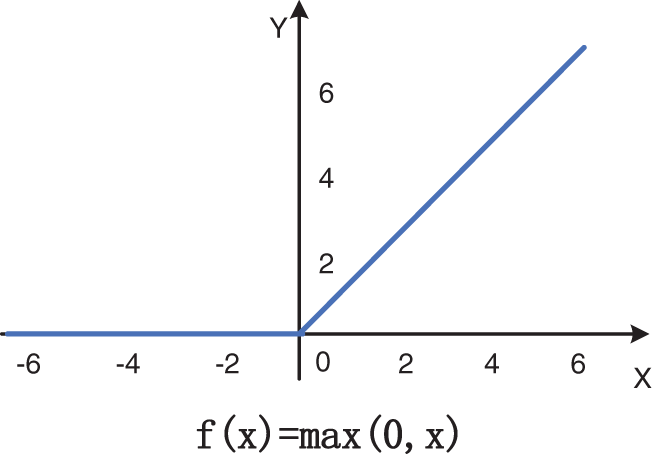
Figure 4: ReLU’s curve and formula

Through a series of improvements, Google proposed an activation function called Swish [39], proving to be more effective than ReLU on deep models. It has the characteristics of unsaturated, smooth, and non-monotone. The formula is as follows:

f(x)=x⋅sigmoid(β~x)(3)

where β~ is a trainable parameter.

3  Proposed Method

3.1 Reference System

A stationary reference system is used in this work. The origin of the reference frame is fixed on the predicted agent at time t. Take vehicle trajectory prediction as an example. As shown in Fig. 5, Y-axis represents the movement direction of the highway, and X-axis is perpendicular to it. Therefore, the model is independent of how the vehicle trajectory is obtained. It also makes the model independent of the curvature of the road. The reference system of pedestrians is similar to that of vehicles.

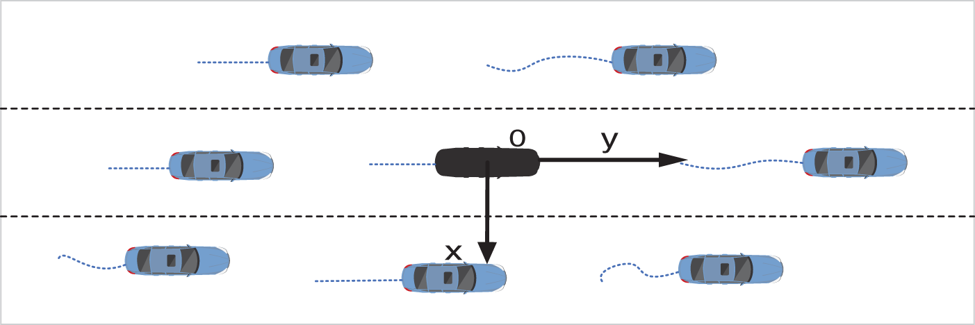
Figure 5: The stationary reference system for vehicle trajectory prediction

3.2 Pipeline of the Proposed Method

We aim to predict the future trajectories of different agents, including vehicles and pedestrians. Specifically, their future trajectories are predicted based on their historical trajectories. Fig. 6 shows the pipeline of the proposed method. After feeding the network with agents’ historical trajectories, it mainly relies on the encoder-decoder structure to capture agents’ motion characteristics and predicts their future trajectories.

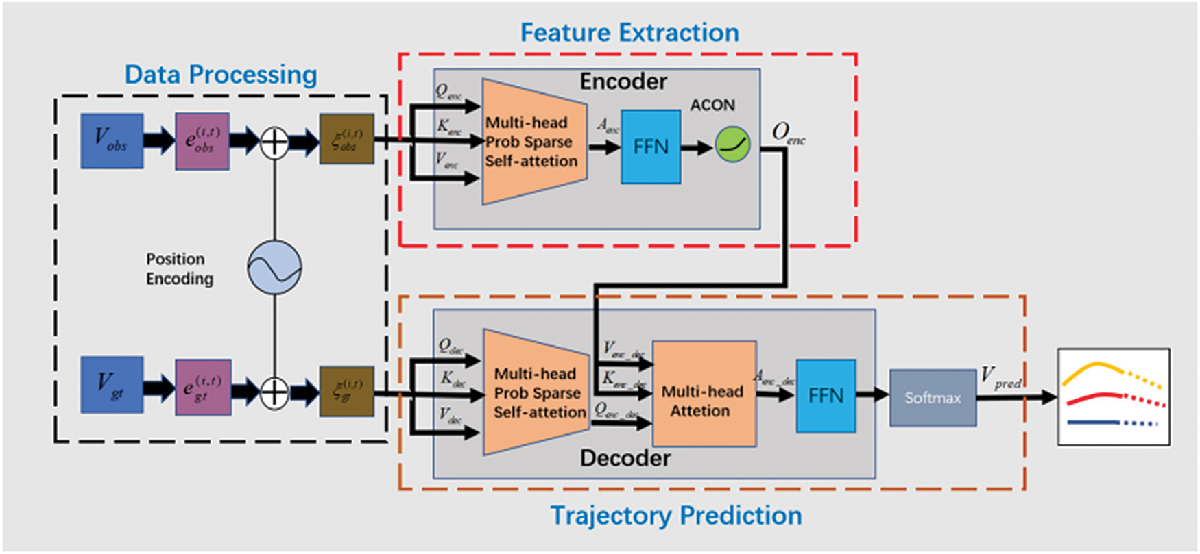
Figure 6: Pipeline of the proposed method

The model is mainly composed of three parts: the data processing part, the feature extraction part, and the trajectory prediction part. Descriptions of different parts are as follows:

Data Processing: For agent i, its historical trajectory is Vobs={xti}t=1Tobs, and the ground truth is Vgt={yti}t=Tobs+1Tpred. As shown in Fig. 6, in order to enable the network to better process the input data, the trajectory information is mapped to a high dimensional space by a linear transformation with learnable weight Wx and Wy, as follows:

eobs(i,t)=xtiWx(4)

egt(i,t)=ytiWy(5)

In Eq. (4), xti represents the historical position, and eobs(i,t) is its embedding obtained through a linear transformation. In Eq. (5), yti represents the ground truth position, and egt(i,t) is its embedding.

To add timing information to the input embedding, the position embedding PE(t,d) is added into the eobs(i,t) and egt(i,t), as follows:

ξobs(i,t)=PE(t,d)+eobs(i,t)(6)

ξgt(i,t)=PE(t,d)+etgt(i,t)(7)

where PE(t,d) will be introduced in Section 3.C. ξobs(i,t)and ξgt(i,t)represent the embedding of the historical and ground truth trajectories with timing information. Finally, ξobs(i,t) is fed into both the encoder and the decoder.

Feature Extraction: After data processing, ξobs(i,t)is fed into the encoder and multiplied by three linear transformations with learnable weights WQenc, WKenc, and WVenc, respectively. Then, three matrices, including the query (Qenc), key (Kenc) and value (Venc), are calculated as follows:

Qenc=WQencξobs(i,t)(8)

Kenc=WKencξobs(i,t)(9)

Venc=WVencξobs(i,t)(10)

Afterward, the sparse self-attention module calculates the first U dot product pairs with high correlation, and then multiplier them with Venc to get the attention matrix Aenc as follows:

U=c∗ln⁡LQenc(11)

Q¯={Qenci}i=0U(12)

Aenc=softmax(Q¯KencTdk)Venc(13)

where c is the constant sampling factor and dk is the dimension of Ku, Q¯ is a sparse matrix with the same size as Qdec, which only contains the first U queries. Section 3.4 will provide a detailed explanation of Eq. (13).

Aenc is then fed into a feed-forward neural network (FFN), which is followed by the ACON activation function for adaptive activation. Finally, the output of the encoder is defined as follows:

Oenc=ACON(FFN(Aenc))(14)

Trajectory Prediction: Trajectory prediction is mainly achieved in the decoder, which predicts future trajectories in an auto-regression manner. The decoder mainly consists of two inputs, the ground truth trajectory embedding ξgt(i,t), and the output of the encoder Oenc. ξgt(i,t) is fed into the decoder and multiplied by three linear transformations with learnable weights WQdec, WKdec, and WVdec, respectively. Then, three matrices, including the query (Qdec), key (Kdec) and value (Vdec), are defined as follows:

Qdec=WQdecξgt(i,t)(15)

Kdec=WKdecξgt(i,t)(16)

Vdec=WVdecξgt(i,t)(17)

Afterward, the multi-head probabilistic sparse self-attention module takes three embeddings as input and outputs the attention matrix Adec as follows:

Adec=softmax(Q¯decKdecTdk)Vdec(18)

where Q¯dec is a sparse matrix with the same size as Qdec, which only contains the first U queries. Notably, an upper triangle mask is used to shield out future trajectory information since it may influence the trajectory forecasting performance. Then, Adec is fed into the encoder-decoder multi-headed attention module, where Qenc_dec = Adec, Kenc_dec = Venc_dec = Adec. The output of the decoder is defined as follows:

Aenc_dec=softmax(Qenc_decKenc_decTdk)Venc_dec(19)

where dk is the dimension of Kenc_dec.

Finally, Aenc_dec is fed into an FFN, which is followed by a Softmax activation function, to generate future trajectories Vpred={x^ti}t=Tobs+1Tpred, as follows:

Vpred=Softmax(FFN(Aenc_dec))(20)

3.3 Position Embedding

The Transformer network could not capture the sequential properties of sequences since it has no loop structure like LSTM. Hence, a position embedding technology [40] is introduced when encoding the input. In this work, the position embedding PE(t,d) used in Eqs.(6) and (7) is calculated based on the sine-cosine rule, as follows:

PE(t,d)={sin⁡(t/10000d/dmodel) when d is evencos⁡(t/10000d/dmodel) when d is odd(21)

where d represents the dimension of the agent’s position vector at time step t.

3.4 Probabilistic Sparse Self-attention Mechanism

In the traditional self-attention, each position of the trajectory needs to pay attention to all other positions. However, the learned attention matrix is very sparse. Therefore, the computation complexity could be reduced by incorporating structural bias to limit the number of query-key pairs that each query attends. Under this restriction, we introduce sparse attention, in which only the similar Q-K pairs are calculated. Then, the complexity of attention could be reduced by decreasing the number of Q, which represents the query prototype.

In this work, several query prototypes are selected as the primary sources to calculate the distribution of attention. The model either copies the distributions to the locations of the represented queries or populates those locations with uniform distributions. Fig. 7 shows the flow chart to calculate the query prototype.

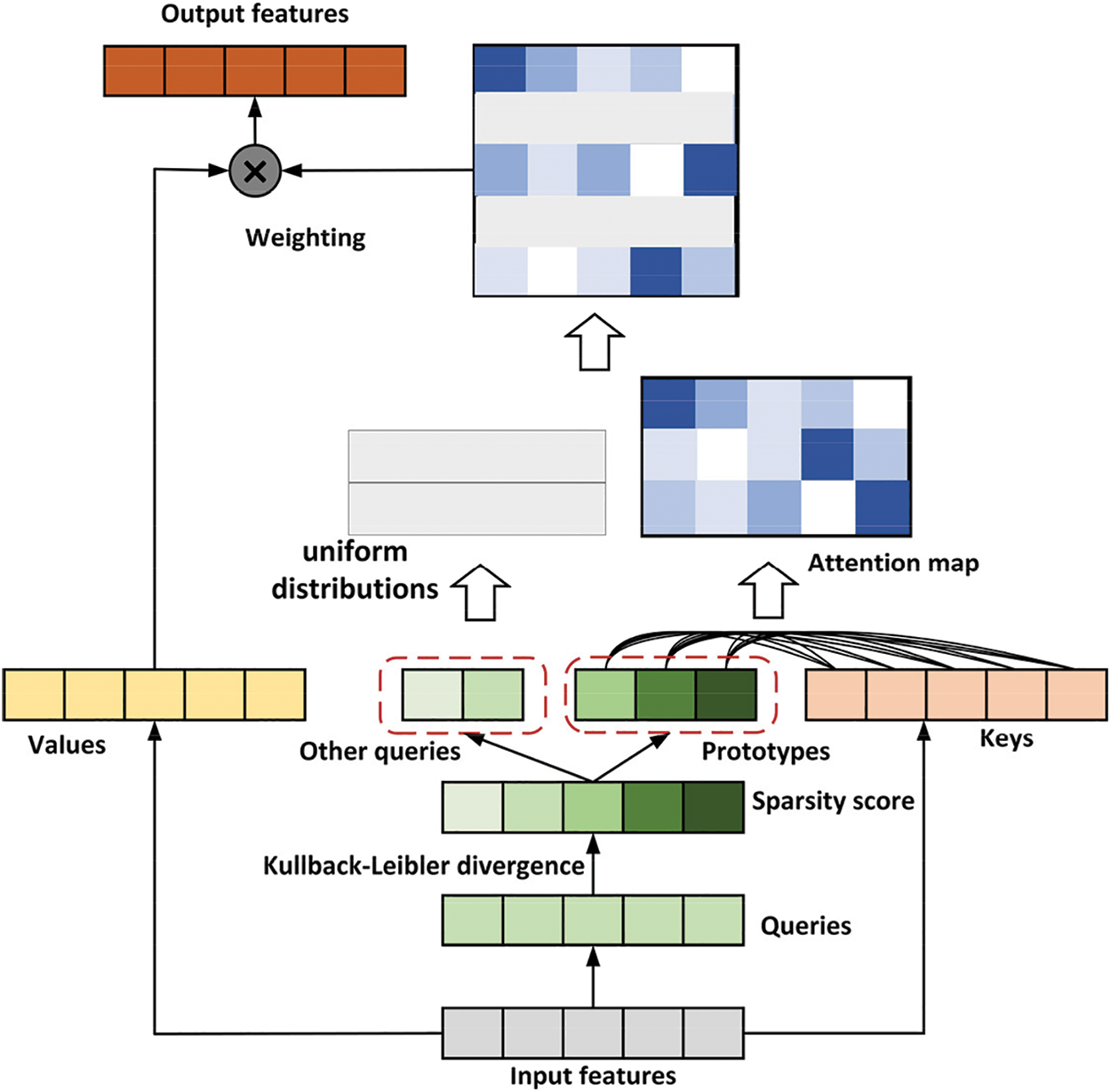
Figure 7: Flow chart of the query prototype

The query sparsity measurement is adopted, and the prototype is selected from the query. The measurement method is the Kullback-Leibler divergence between the attention distribution of the query and the discrete uniform distribution. We define the ith query’s sparsity measurement as:

M(qi,K)=ln⁡∑j=1LKeqikjTd−1LK∑j=1LKqikjTd(22)

The first term is the log-sum-exp (LSE) of qi over all keys, and the second term is their arithmetic means. If the ith query obtains a larger M(qi, K), then its attention probability p is more diversified and has a higher probability that contains the dominant dot product pairs in the head domain of the long-tailed self-attention distribution.

Based on the above discussions, the sparse self-attention [25] only allows each key to process U dominant queries, and its formula is as follows:

A(Q,K,V)=Softmax(Q¯KTd)V(23)

where Q¯ is a sparse matrix with the same size as q, which only contains the first U queries under the sparse metric M(q, k). Controlled by a constant sampling factor c, we set u = c*lnLQ, which makes the Prob Sparse self-attention only need to calculate O(lnLQ) dot-product for each query-key lookup and the layer memory usage maintains O(LKlnLQ).

3.5 ACON Activation Function

Ma et al. [27] presented that Swish is a smooth approximation of ReLU. A new activation function ACON, is proposed to determine whether to activate or not based on Swish adaptively. The most extensive form is ACON-C, and the calculation is as follows:

f(x)=(p1−p2)xσ[β(p1−p2)x]+p2⋅x(24)

where p1 and p2 are two learnable parameters, and β is a switching coefficient. Notably, ACON-C is simple and does not add any computing overhead.

3.6 Loss Function

The loss function [41] is the critical factor in training a deep neural network. The L2 loss function is adopted in this work to calculate the error between ground truth positions and predicted positions of agents’ trajectories. The L2 loss is calculated as follows:

L(Vgt,Vpred)=1Tpred∑t=1Tpred(yti−x^ti)2(25)

where yti and x^ti are positions in ground truth and predicted trajectories, respectively. Tpred represents the predicted time steps.

4  Experimental Results

4.1 Datasets

The proposed method is evaluated on two publicly available benchmarks, namely next-generation simulation (NGSIM) and ETH/UCY datasets. The former one contains vehicles’ trajectories, and the latter one contains pedestrians’ trajectories. Their details are introduced as follows:

NGSIM: NGSIM [42,43] is a traffic dataset collected on American highways. It contains two scenes, US-101 and I80. For each scene, all vehicles’ trajectories are recorded over 45 min and with a sampling frequency of 10 Hz. It is divided into three 15-min segments under mild, moderate, and congested traffic conditions, respectively. In this work, we split all the trajectories contained in NGSIM, in which 70% are used for training, 20% are used for testing, and the left 10% are used for validation. Each trajectory is split into an 8s segment, consisting of 3s historical trajectory and 5s future trajectory (used as ground truth). We down-sample the original frequency of 10 to 5Hz. Hence, 15 historical positions and 25 ground truth positions are obtained in each trajectory.

ETH/UCY: This dataset includes a total of 5 videos (ETH, HOTEL, UNIV, ZARA1, and ZARA2) from 4 different scenes (ZARA1 and ZARA2 from the same camera, but at different times) [44]. Totally 1536 pedestrians are in the crowds with challenging social interactions. According to the evaluation protocol, samples are taken from the data every 0.4 s to generate the trajectory. The pedestrian position is converted from the original pixel positions to meters in real-world coordinates using the homology matrix. We use the leave-one-out approach for fair comparisons, train on four sets, and test on the remaining set. We observe each trajectory for 3.2 s (8 frames) and obtain the next 4.8 s (12 frames) of ground truth data.

4.2 Metrics

Average Displacement Error (ADE) and Final Displacement Error (FDE) are used as metrics for evaluation. ADE is used to measure the average difference at each time step between the predicted trajectory and the ground truth. FDE is used to measure the distance between the final destinations of the predicted trajectory and the ground truth.

4.3 Experimental Details

The experimental environment used is the Ubuntu system and the PyTorch framework. The Adam optimizer is used to train the network with a learning rate of 0.0004. The dropout value is set as 0.1. Other hyper-parameters, including the training epochs, the layer numbers, the embedding size, and the head numbers used in the Transformer network, are fine-tuned through cross-validations on the ETH/UCY databases.

4.4 Hyper-Parameter Fine-tuning

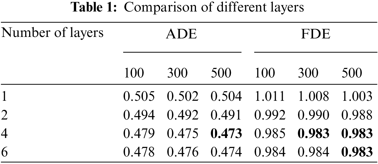
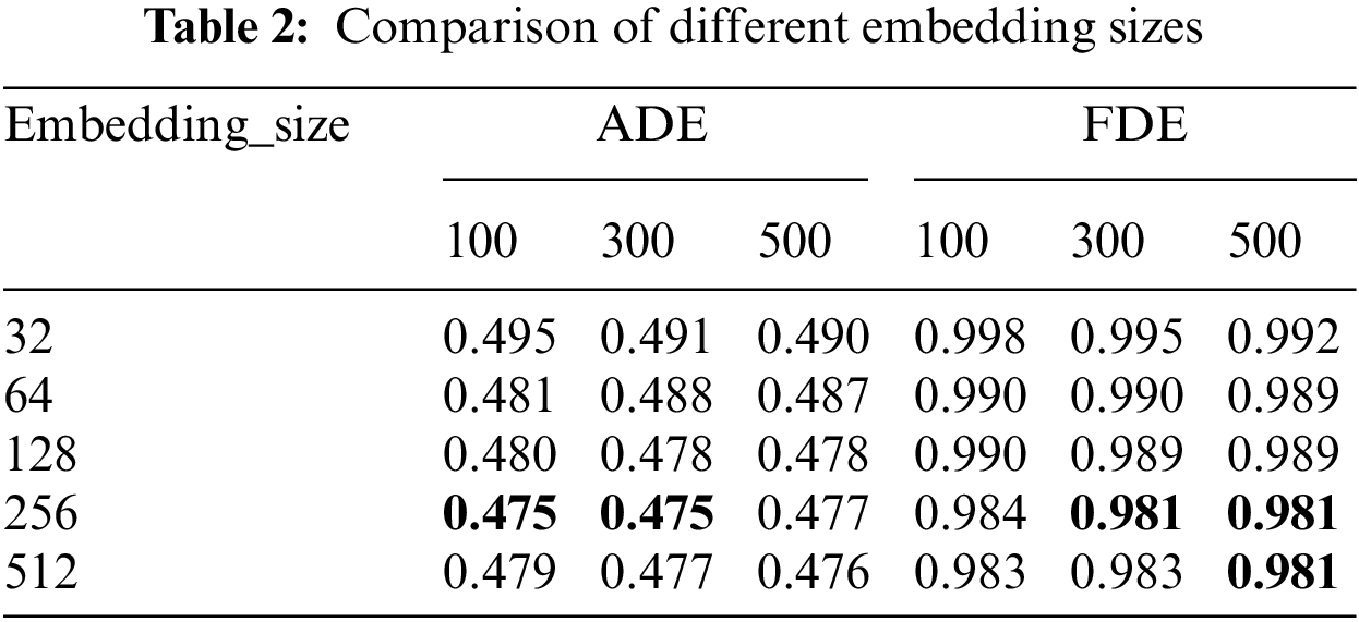
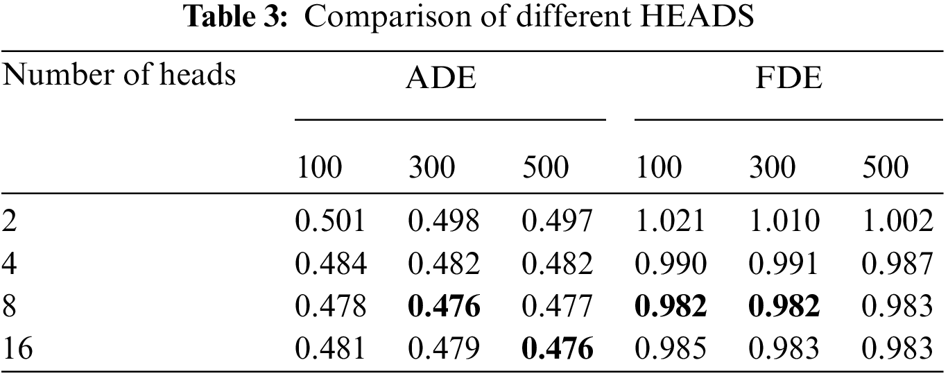
Unlike LSTM-based trajectory prediction methods, the Transformer network has a large space-time overhead. Hence, hyper-parameter fine-tuning is performed on the ETH/UCY database, which contains much fewer trajectories than NGSIM. Specifically, we evaluate the proposed method on the ETH/UCY when using different layer numbers, embedding sizes, head numbers, and different training epochs (100, 300, 500). The initial values of the layer numbers, embedding sizes, and head numbers are empirically set to 4, 128, and 8, respectively. We fix other hyper-parameters when we fine-tune a certain hyper-parameter.

Tabs. 1–3 report the average ADE/FDE values on ETH/UCY using different hyper-parameters of the Transformer network. It is obvious that the proposed method could achieve the best performance on the ETH/UCY when setting the layer number to 4, the embedding size to 256, and the head number to 8. Besides, we find that the training epochs (100, 300, 500) would not greatly influence the trajectory prediction performance. However, a large training epoch will greatly increase the training time. Hence, we set the training epoch to 100 for efficient training.

4.5 Ablation Study

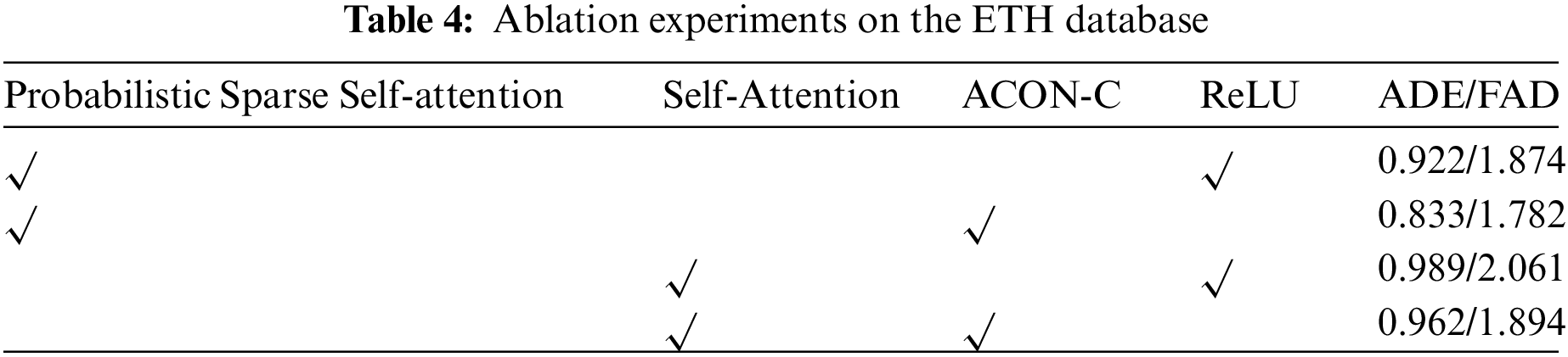
The main contribution of this paper is to replace the traditional self-attention mechanism with the probabilistic sparse self-attention mechanism, which significantly reduces the space-time complexity of the model and improves efficiency. Besides, the ACON-C activation function is used to adjust whether to activate or not adaptively. We perform a detailed ablation study on two benchmarks to exhibit the effects of the proposed improvements. Specifically, we compare the trajectory prediction performance between the probabilistic sparse self-attention and the traditional self-attention. We also compare the performance between the ReLU and the ACON-C. As indicated by Tab. 4, better performance is achieved by replacing the traditional ReLU and self-attention with ACON-C and the probabilistic sparse self-attention, which reveals the effects of the proposed improvements.

4.6 Quantitative Evaluations

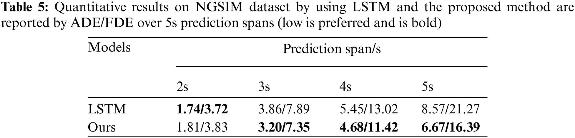
In this work, an improved Transformer network is proposed to perform trajectory for both vehicles and pedestrians. Firstly, we evaluate the influence of prediction spans on vehicle trajectory prediction. Tab. 5 presents the quantitative results on NGSIM dataset by ADE/FDE over 5s prediction spans. We use the LSTM-based trajectory prediction method for comparison. As shown in the table, the LSTM-based method performs well in a short period (2s). However, its performance gradually deteriorates with the increase of the predicted sequence length. Such results indicate that the LSTM sequential processing structure performs poorly in modeling complex and large amounts of data and has limited ability to process long sequences. Unlike LSTM, the Transformer network could learn from all moments in parallel, thus improve efficiency and scalability.

To further demonstrate the effects of the proposed method, we make a quantitative analysis by comparing the proposed method with several state-of-the-art methods, including the LSTM-based method, Social-LSTM [19], SGAN [45], and Sophie [46]. Social-LSTM presents the social pooling layer to capture social interactions. SGAN introduces an adversarial training manner to generate future trajectories. Sophie proposes social and physical attention modules to improve the predicted trajectories. For NGSIM, we compare the trajectory prediction performance by generating the future trajectories within the 5s prediction span. As shown in Tab. 6, although Sophie has a better effect on I80 moderately dense scenario, the proposed method achieves better performance on other scenes compared with other methods. Besides, the proposed method achieves the lowest average ADE/FDE.

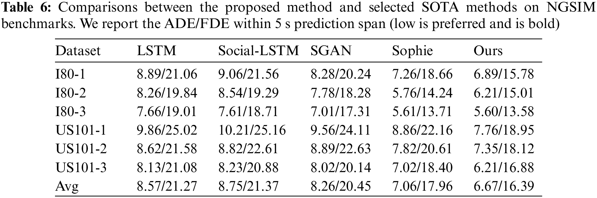
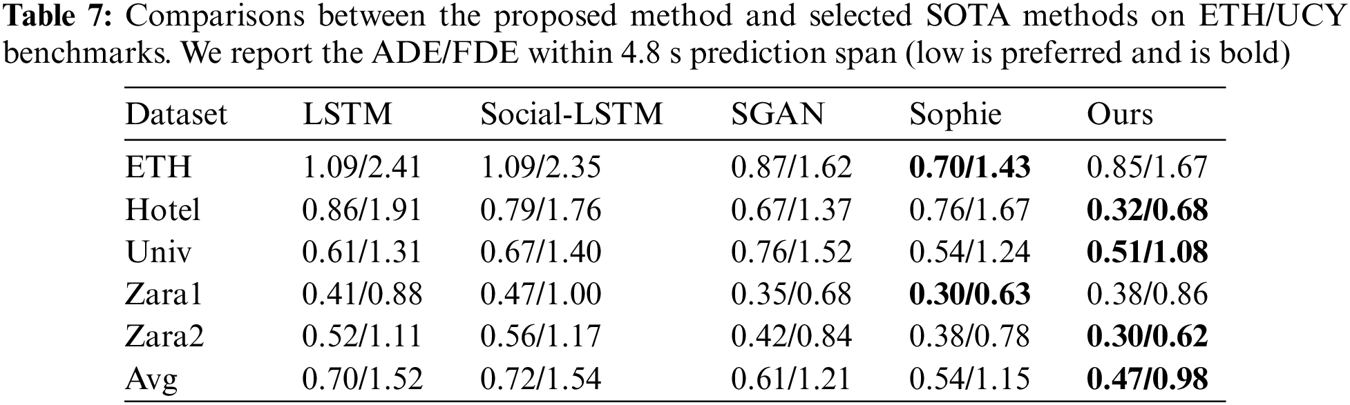
For comparisons on ETH/UCY as shown in Tab. 7, it is evident that the proposed method is superior to other methods, especially in the term of average ADE/FDE. Compared with SGAN, our method achieves better trajectory prediction performance on all five scenes. Compared with Sophie, our method achieves better trajectory prediction performance on Hotel, Univ, and Zara2 scenes. Such a superiority reveals the effects of the improved Transformer network in capturing the temporal association of the trajectory data.

4.7 Qualitative Analysis

We perform the qualitative analysis to demonstrate the effects of the proposed method. Figs. 8a and 8b exhibit the trajectory prediction performance using the proposed method and an LSTM-based method on the NGSIM and ETH, respectively. The red line represents the historical trajectory, the blue line represents the ground truth trajectory, the green line represents the trajectory predicted by the proposed method, and the yellow line represents the trajectory predicted by the LSTM-based method. The over-fitting phenomenon exists in the LSTM-based method. As shown in the 4th sub-figure of Fig. 8b, even if the vehicle travels in a straight line, its prediction tends to bend in one direction. Besides, as shown in the 4th sub-figure of Fig. 8a, when a vehicle suddenly makes a big turn, the model cannot predict the future trajectory based on the historical trajectory of the vehicle position. Therefore, environmental factors need to be added in order to have a more accurate prediction of emergencies.

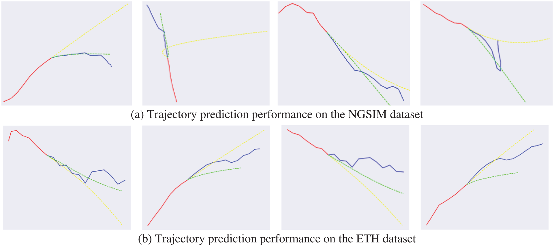
Figure 8: Trajectory prediction performance by using the proposed method and an LSTM-based method, respectively. The red line represents the historical trajectory, the blue line represents the ground truth trajectory, the green line represents the trajectory predicted by the proposed method, and the yellow line represents the trajectory predicted by the LSTM-based method

In this work, Gaussian noise is added to the model to simulate some uncertain factors. After that, vehicles’ predicted trajectories are more polymorphic than before. As shown in Fig. 9a, more traffic conditions can be simulated with the help of the added Gaussian noise. In Fig. 9b, we can observe that the distributions of the generated trajectories conform to the two-dimensional Gaussian distribution. Afterward, we compare the trajectory prediction performance of the proposed method on NGSIM w/o Gaussian noise. As demonstrated in Fig. 10, after adding noise, it can be seen that the generated multiple trajectories are better than those without noise. Such results indicate that the addition of noise improves the model’s accuracy and makes the model diversified.

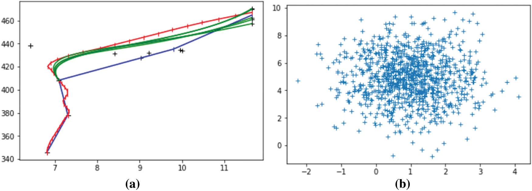
Figure 9: In the left figure, red rep resents the real trajectory of the vehicle, blue represents the trajectory generated on the verification set without adding noise, and green represents the trajectory generated after adding noise. The figure on the right is a two-dimensional Gaussian distribution scatter diagram of the trajectory

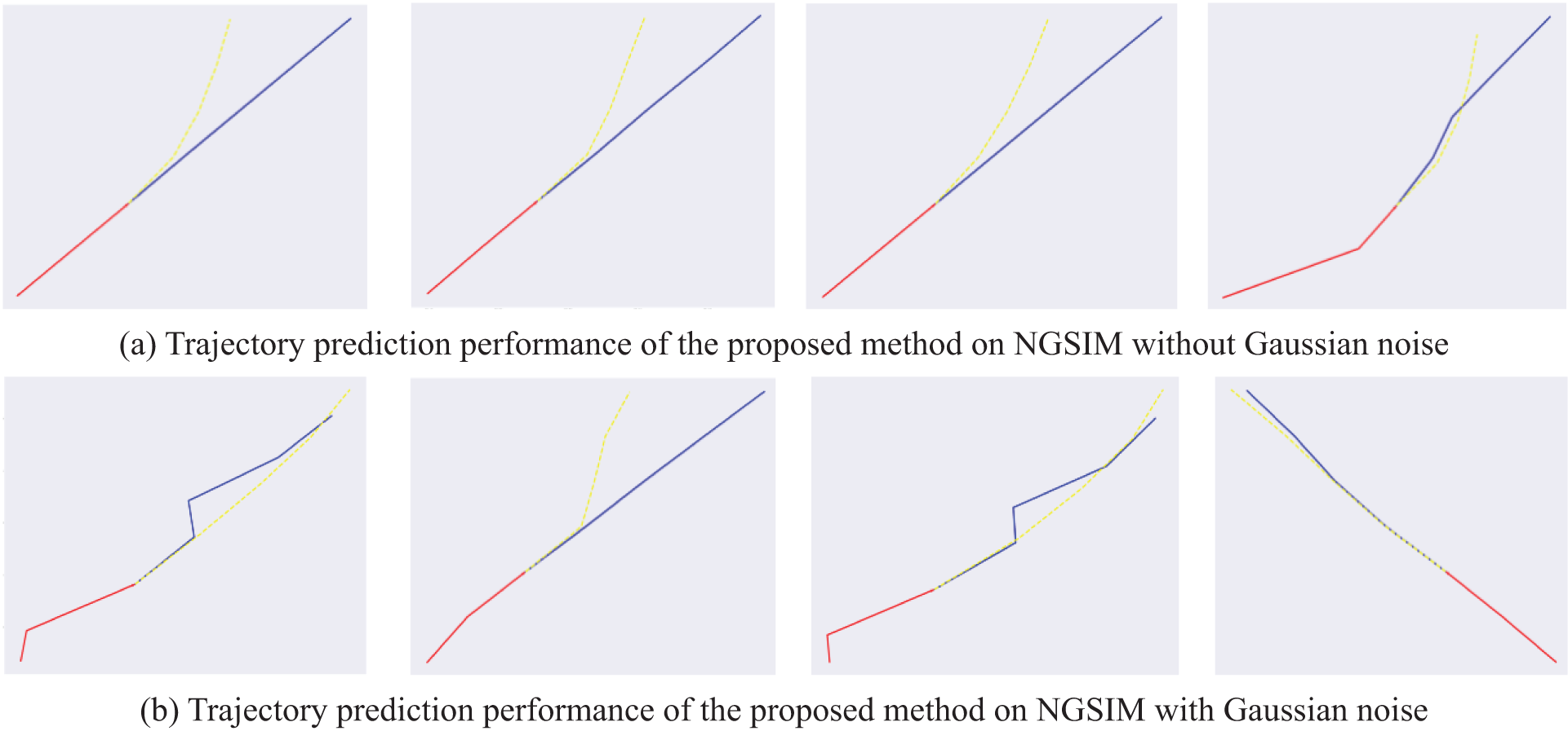
Figure 10: Trajectory prediction performance of the proposed method on NGSIM w/o Gaussian noise. The red line represents the historical trajectory, the blue line represents the ground truth trajectory, and the yellow line represents the trajectory predicted by the proposed method

5  Conclusion and Discussion

An improved Transformer network is proposed to perform trajectory prediction in this work. A traditional Transformer network utilizes the multi-head attention mechanism to capture sequential information in agents’ trajectories. It exhibits better performance than the LSTM-based trajectory prediction methods. Further, a probabilistic sparse self-attention mechanism is introduced to solve the problems of attention query sparsity and the high space-time complexity in the self-attention mechanism. The ACON activation function is used to solve the problem that traditional activation functions are sensitive to parameter initialization, learning rate, and neuron death. Evaluations on publicly available NGSIM and ETH/UCY indicate that the proposed method is suitable to forecast future trajectories of vehicles and pedestrians. Our future works mainly focus on recognizing pedestrians’ crossing intentions [47] or vehicle re-identification [48] with the predicted trajectories.

Funding Statement: This work has been supported by the Suzhou Key industrial technology innovation project SYG202031.This work has been supported by the Future Network Scientific Research Fund Project,FNSRFP-2021-YB-29.

Conflicts of Interest: The authors declare that they have no conflicts of interest to report regarding the present study.

References

 1.  Y. F. Cai, L. Dai, H. Wang, L. Chen, Y. C. Li et al., “Pedestrian motion trajectory prediction in intelligent driving from far shot first-person perspective video,” IEEE Transactions on Intelligent Transportation Systems, vol. 23, no. 6, pp. 5298–5313, 2022. [Google Scholar]

 2.  W. Sun, L. Dai, X. R. Zhang, P. S. Chang and X. Z. He, “RSOD: Real-time small object detection algorithm in UAV-based traffic monitoring,” Applied Intelligence, vol. 92, no. 6, pp. 164, 2021. [Google Scholar]

 3.  X. R. Zhang, X. Sun and W. Sun, “Deformation expression of soft tissue based on BP neural network,” Intelligent Automation & Soft Computing, vol. 32, no. 2, pp. 1041–1053, 2022. [Google Scholar]

 4.  X. R. Zhang, W. F. Zhang and W. Sun, “A robust 3-D medical watermarking based on wavelet transform for data protection,” Computer Systems Science & Engineering, vol. 41, no. 3, pp. 1043–1056, 2022. [Google Scholar]

 5.  X. R. Zhang, X. Sun and X. M. Sun, “Robust reversible audio watermarking scheme for telemedicine and privacy protection,” Computers, Materials & Continua, vol. 71, no. 2, pp. 3035–3050, 2022. [Google Scholar]

 6.  C. Shen, Y. Zhang, X. Guo, X. Y. Chen, H. L. Cao et al., “Seamless GPS/inertial navigation system based on self-learning square-root cubature Kalman filter,” IEEE Transactions on Industrial Electronics, vol. 68, no. 1, pp. 499–508, 2020. [Google Scholar]

 7.  C. Shen, Y. Xiong, D. Zhao, C. G. Wang, H. L. Cao et al., “Multi-rate strong tracking square-root cubature Kalman filter for MEMS-INS/GPS/polarization compass integrated navigation system,” Mechanical Systems and Signal Processing, vol. 163, no. 108146, pp. 108146, 2022. [Google Scholar]

 8.  B. Yang, G. Yan, P. Wang, C. Y. Chan, X. Song et al., “A novel graph-based trajectory predictor with pseudo-oracle,” IEEE Transactions on Neural Networks and Learning Systems, Early Access, 2021. https://doi.org/10.1109/TNNLS.2021.3084143. [Google Scholar]

 9.  C. He, L. Chen, L. Xu, C. Yang, X. F. Liu et al., “IRLSOT: Inverse reinforcement learning for scene-oriented trajectory prediction,” IET Intelligent Transport Systems, vol. 16, no. 6, pp. 769–781, 2022. [Google Scholar]

10. C. He, B. Yang, L. Chen and G. C. Yan, “An adversarial learned trajectory predictor with knowledge-rich latent variables,” in Chinese Conf. on Pattern Recognition and Computer Vision (PRCV), Xi’an, China, pp. 42–53, 2020. [Google Scholar]

11. A. Houenou, P. Bonnifait, V. Cherfaoui and W. Yao, “Vehicle trajectory prediction based on motion model and maneuver recognition,” in IEEE/RSJ Int. Conf. on Intelligent Robots & Systems, Tokyo, Japan, pp. 4363–4369, 2013. [Google Scholar]

12. X. Ji, C. Fei, X. He, Y. Liu and Y. H. Liu, “Intention recognition and trajectory prediction for vehicles using LSTM network,” China Highway and Transportation, vol. 32, no. 6, pp. 34–42, 2019. [Google Scholar]

13. X. R. Zhang, J. Zhou and W. Sun, “A lightweight CNN based on transfer learning for COVID-19 diagnosis,” Computers, Materials & Continua, vol. 72, no. 1, pp. 1123–1137, 2022. [Google Scholar]

14. B. Yang, J. M. Cao, N. Wang and X. F. Liu, “Anomalous behaviors detection in moving crowds based on a weighted convolutional autoencoder-long short-term memory network,” IEEE Transactions on Cognitive and Developmental Systems, vol. 11, no. 4, pp. 473–482, 2018. [Google Scholar]

15. Z. Zhao, W. Chen, X. Wu, P. C. Chen and J. Liu, “LSTM network: A deep learning approach for short-term traffic forecast,” IET Intelligent Transport Systems, vol. 11, no. 2, pp. 68–75, 2017. [Google Scholar]

16. A. Khosroshahi, E. Ohn-Bar and M. M. Trivedi, “Surround vehicles trajectory analysis with recurrent neural networks,” in 2016 IEEE 19th Int. Conf. on Intelligent Transportation Systems (ITSC), Rio de Janeiro, Brazil, pp. 2267–2272, 2016. [Google Scholar]

17. D. J. Phillips, T. A. Wheeler and M. J. Kochenderfer, “Generalizable intention prediction of human drivers at intersections,” in 2017 IEEE Intelligent Vehicles Symp. (IV), Los Angeles, CA, USA, pp. 1665–1670, 2017. [Google Scholar]

18. B. D. Kim, C. M. Kang, J. Kim, S. H. Lee, C. C. Chung et al., “Probabilistic vehicle trajectory prediction over occupancy grid map via recurrent neural network,” in 2017 IEEE 20th Int. Conf. on Intelligent Transportation Systems (ITSC), Yokohama, Japan, pp. 399–404, 2017. [Google Scholar]

19. A. Alahi, K. Goel, V. Ramanathan, A. Robicquet, F. F. Li et al., “Social LSTM: Human trajectory prediction in crowded spaces,” in Proc. of the IEEE Conf. on Computer Vision and Pattern Recognition, New York, NY, USA, pp. 961–971, 2016. [Google Scholar]

20. J. Devlin, M. W. Chang, K. Lee and K. Toutanova, “Bert: Pre-training of deep bidirectional transformers for language understanding,” 2018. [Online]. Available: https://arxiv.org/abs/1810.04805. [Google Scholar]

21. Z. Lan, M. Chen, S. Goodman, K. Gimpel, P. Sharma et al., “Albert: A lite bert for self-supervised learning of language representations,” 2019. [Online]. Available: https://arxiv.org/abs/1909.11942. [Google Scholar]

22. R. Child, S. Gray, A. Radford and I. Sutskever, “Generating long sequences with sparse transformers,” 2019. [Online]. Available: https://arxiv.org/abs/1904.10509. [Google Scholar]

23. W. Sun, X. Chen and X. R. Zhang, “A multi-feature learning model with enhanced local attention for vehicle re-identification,” Computers, Materials & Continua, vol. 69, no. 3, pp. 3549–3561, 2021. [Google Scholar]

24. C. Yu, X. Ma, J. Ren, H. Zhao and S. Yi, “Spatio-temporal graph transformer networks for pedestrian trajectory prediction,” in European Conf. on Computer Vision, Cham, Springer, pp. 507–523, 2020. [Google Scholar]

25. H. Zhou, S. Zhang, J. Peng, S. Zhang, J. Li et al., “Informer: Beyond efficient transformer for long sequence time-series forecasting,” in Proc. of AAAI, Electr Network, pp. 11106–11115, 2021. [Google Scholar]

26. N. Kitaev, L. Kaiser and A. Levskaya, “Reformer: The efficient transformer,” 2020. [Online]. Available: https://arxiv.org/abs/2001.04451. [Google Scholar]

27. N. Ma, X. Zhang, M. Liu and J. Sun, “Activate or not: Learning customized activation,” in Proc. of the IEEE/CVF Conf. on Computer Vision and Pattern Recognition, New York, NY, USA, pp. 8032–8042, 2021. [Google Scholar]

28. K. Ahmed, N. S. Keskar and R. Socher, “Weighted transformer network for machine translation,” 2017. [Online]. Available: https://arxiv.org/abs/1711.02132. [Google Scholar]

29. Y. Pan, B. Song, N. Luo, X. Chen and H. Cui, “Transformer and multi-scale convolution fortarget-oriented sentiment analysis,” in Asia-Pacific Web (APWeb) and Web-Age Information Management (WAIM) Joint Int. Conf. on Web and Big Data, Cham, Springer, pp. 310–321, 2019. [Google Scholar]

30. P. Li, P. Zhong, J. Zhang and K. Mao, “Convolutional transformer with sentiment-aware attention for sentiment analysis,” in 2020 Int. Joint Conf. on Neural Networks (IJCNN), Glasgow, UK, pp. 1–8, 2020. [Google Scholar]

31. L. Gong, J. M. Crego and J. Senellart, “Enhanced transformer model for data-to-text generation,” in Proc. of the 3rd Workshop on Neural Generation and Translation, Hong Kong, pp. 148–156, 2019. [Google Scholar]

32. K. Cho, B. Van Merriënboer, C. Gulcehre, D. Bahdanau, F. Bougares et al., “Learning phrase representations using RNN encoder-decoder for statistical machine translation,” 2014. [Online]. Available: https://arxiv.org/abs/1406.1078. [Google Scholar]

33. X. Zhang, J. Su, Y. Qin, Y. Liu, R. Ji et al., “Asynchronous bidirectional decoding for neural machine translation,” Proc. of the AAAI Conf. on Artificial Intelligence, vol. 32, no. 1, pp. 5698–5705, 2018. [Google Scholar]

34. H. Fukui, T. Hirakawa, T. Yamashita and H. Fujiyoshi, “Attention branch network: Learning of attention mechanism for visual explanation,” in Proc. of the IEEE/CVF Conf. on Computer Vision and Pattern Recognition, Long Beach, CA, USA, pp. 10705–10714, 2019. [Google Scholar]

35. W. Sun, G. Z. Dai, X. R. Zhang, X. Z. He and X. Chen, “TBE-Net: A three-branch embedding network with part-aware ability and feature complementary learning for vehicle re-identification,” IEEE Transactions on Intelligent Transportation Systems, pp. 1–13, 2021. https://doi.org/10.1109/TITS.2021.3130403 [Google Scholar]

36. Y. F. Cai, L. Dai, H. Wang, L. Chen and Y. C. Li, “DLnet with training task conversion stream for precise semantic segmentation in actual traffic scene,” IEEE Transactions on Neural Networks and Learning Systems, Early Access, 2021. https://doi.org/10.1109/TNNLS.2021.3080261. [Google Scholar]

37. F. Zhang and Z. Zeng, “Multistability and instability analysis of recurrent neural networks with time-varying delays,” Neural Networks, vol. 97, pp. 116–126, 2018. [Google Scholar]

38. K. Eckle and J. Schmidt-Hieber, “A comparison of deep networks with ReLU activation function and linear spline-type methods,” Neural Networks, vol. 110, no. 2–3, pp. 232–242, 2019. [Google Scholar]

39. P. Ramachandran, B. Zoph and Q. V. Le, “Searching for activation functions,” 2017. [Online]. Available: https://arxiv.org/abs/1710.05941. [Google Scholar]

40. X. Wu, Q. Chen, J. You and Y. Xiao, “Unconstrained offline handwritten word recognition by position embedding integrated resnets model,” IEEE Signal Processing Letters, vol. 26, no. 4, pp. 597–601, 2019. [Google Scholar]

41. X. Wang, S. Wang, C. Chi, S. Zhang and T. Mei, “Loss function search for face recognition,” in Int. Conf. on Machine Learning, Seattle, USA , pp. 10029–10038, 2020. [Google Scholar]

42. V. Alexiadis, J. Colyar, J. Halkias and R. Hranac, “The next generation simulation program,” ITE journal, vol. 74, no. 8, pp. 22–26, 2004. [Google Scholar]

43. B. Coifman and L. Li, “A critical evaluation of the Next Generation Simulation (NGSIM) vehicle trajectory dataset,” Transportation Research Part B: Methodological, vol. 105, no. 4, pp. 362–377, 2017. [Google Scholar]

44. S. Pellegrini, A. Ess and L. V. Gool, “Improving data association by joint modeling of pedestrian trajectories and groupings,” in European conf. on Computer Vision, Berlin, Heidelberg, Springer, pp. 452–465, 2010. [Google Scholar]

45. A. Gupta, J. Johnson, F. F. Li, S. Silvio and A. Alexandre, “Social GAN: Socially acceptable trajectories with generative adversarial networks,” in Proc. of the IEEE Conf. on Computer Vision and Pattern Recognition, Salt Lake City, USA, pp. 2255–2264, 2018. [Google Scholar]

46. A. Sadeghian, V. Kosaraju, A. Sadeghian, N. Hirose, H. Rezatofighi et al., “An attentive gan for predicting paths compliant to social and physical constraints,” in Proc. of the IEEE/CVF Conf. on Computer Vision and Pattern Recognition, Long Beach, USA, pp. 1349–1358, 2019. [Google Scholar]

47. B. Yang, W. Zhan, P. Wang, C. Chan, Y. F. Cai et al., “Crossing or not? Context-based recognition of pedestrian crossing intention in the urban environment,” IEEE Transactions on Intelligent Transportation Systems, vol. 23, no. 6, pp. 5338–5349, 2022. [Google Scholar]

48. X. R. Zhang, X. Chen and W. Sun, “Vehicle re-identification model based on optimized densenet121 with joint loss,” Computers, Materials & Continua, vol. 67, no. 3, pp. 3933–3948, 2021. [Google Scholar]