Optimal Deep Transfer Learning Based Colorectal Cancer Detection and Classification Model

1  Introduction

Colorectal cancer (CRC) is the second most typical reason for cancer death rate in America and Europe [1]. Pathological diagnosis was considered the most authorized technique for treating CRC that needs pathologist personnel to visibly scrutinize digital full scale whole slide images (WSI) [2]. The challenges stem from the difficulty of WSI comprising large images, histological alterations, textures, and complex shapes in nuclear staining [3]. In addition to this, lacking pathologists globally is in stark contrast to the fast collection of WSI data, and the daily work pressure of pathologists is intense which results in unintended misdiagnose because of exhaustion. Therefore, it is important to enhance diagnosing methodologies that are cost effective by using current artificial intelligence (AI) advancements [4].

Pathology slides offer a numerous quantity of data that was measured by traditional machine learning (ML) methods and digital pathology for years [5]. The earlier study was depending on ML methods for determining the cell classifier from the histological slides of tumor tissue. The categorization of histopathological images by using AI not only escalates the efficiency and preciseness of the classification but also allows doctors in taking prompt actions about clinical treatment [6]. But, many of the suggested simulation practices depends on manual feature labels, which consider the primary constraints of conventional textual analysis methods. Thus, in the past few years, deep learning (DL) was inaugurated for solving this issue and other restrictions [7].

DL is a new technology that acts as an advancement of machine learning, but then it utilizes various layers of neural network (NN) systems for learning and increasingly abstracts high level features to minimize the intervention of humans from the identification of distinct classes in the images [8]. Traditional neural networks (CNN) currently present proficient outcomes in classifying images in the domain of DL whereas a NN may have hundreds or dozens of layers for learning comprising images with distinct features [9]. A convolutional layer made up of a small sized kernel to produce enriched features implies weights to the input unit and instructs them via an activation function as the output unit. The primary benefit of utilizing CNN in comparison made to a classic NN is that it minimizes the model variables for better precise outcomes [10].

The researchers in [11] present a novel dynamic ensemble DL technique. Firstly, it produces a subset of methods according to the transfer learning approach in deep neural network (DNN). Next, the applicable set of methods is carefully chosen by the particle swarm optimization approach and integrated by averaging or voting systems. Sarwinda et al. [12] examine a DL technique in image classification for detecting CRC using ResNet framework. The excellent achievement of a DL classifier method provokes scholars to perform them in medicinal images. The model trained to differentiate CRC into malignant and benign cancer. Mulenga et al. [13] presented a feature augmentation method that groups data normalization method to prolong current feature of data. The projected technique integrates feature extension by augmenting information for improving CRC classifier accuracy of DNN architecture.

Ho et al. [14] encompass a deep learning method based Fast Region related Convolution Neural Network (Fast-RCNN) structure for occurrence segmentation with a ResNet-101 feature extraction support which offers glandular segmentation, as well as traditional ML classification. Tsai et al. [15] presented the optimal classifier method based selected optimizer and adapted the parameter of CNN method. Next, we employed DL method for differentiating between diseased and healthy large intestine tissues. Initially, we trained a NN and related the network structure optimizer. Next, it can be adapted the parameter of the network layer to augment the better structure. At last, we compared the highly trained DL method on two distinct histological image open data sets.

This study develops a slime mould algorithm with deep transfer learning enabled colorectal cancer detection and classification (SMADTL-CCDC) approach. The presented SMADTL-CCDC technique undergoes pre-processing to improve the input image quality. In addition, a dense-EfficientNet method was employed to extract feature vectors from the pre-processed images. Moreover, SMA with Discrete Hopfield neural network (DHNN) approach was applied for the recognition and classification of CRC. The utilization of SMA assists in appropriately selecting the parameters involved in the DHNN approach. A wide range of experiments was applied to benchmark datasets for assessing the classification performances.

The rest of the paper is provided as follows. Section 2 offers the proposed model and Section 3 provides performance validation. Lastly, Section 4 concludes the work.

2  The Proposed Model

In this study, a new SMADTL-CCDC model has been developed to appropriately recognize the occurrence of CRC. The SMADTL-CCDC model originally undergoes pre-processing to improve the input image quality. Followed by, a dense-EfficientNet model is employed to extract feature vectors in the pre-processed images. Moreover, SMA with DHNN model is applied for the recognition and classification of CRC. Fig. 1 illustrates the work flow of SMADTL-CCDC technique.

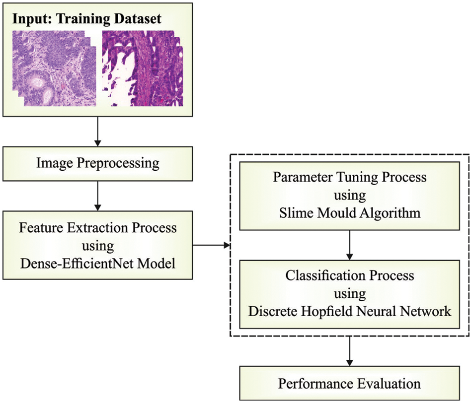
Figure 1: Work flow of SMADTL-CCDC technique

2.1 Feature Extraction

Once the medical image is preprocessed, the next step is for deriving a set of feature vectors using the dense EfficientNet model. CNN contains a group of layers implemented from the finding of image features. One of the important layers is pooling, convolution, activation, and batch normalization (BN) layers. Primary, the convolution layer is considered that needed unit from the CNN frameworks. The layer has contained a group of filters for discovering the existence of specific features which is executed from the image characterized as edge and texture called feature maps. Afterward, the activation layer is utilized for processing non-linear transformation for determining the result of prior convolution layer with application of activation function, for instance, Rectified Linear Unit (ReLU). The ReLU has generally utilized the activation function as it offers fast processing and demonstrations no problem with exploding problems. The ReLU is formulated as:

F(x)=max(0,x).(1)

whereas the gradient for input is determined as:

∂F(x)∂x={0 ifx≤01 ifx>0(2)

The BN layer tries for minimizing the amount of trained epochs that are needed from the network trained. It also improves the function by rescaling all the scalar features xu with restricted mini-batch B={x1,m} dependent upon Eq. (3)

x^u=xu−μBσB2+ε(3)

In which ε signifies the smaller positive value for terminating the division by 0, μB represents the mini-batch mean that is defined with utilize of Eq. (4), and σB2 stands for the mini-batch variance that is evaluated by Eq. (5).

μB=1m∑u=1mxv(4)

σB2=1m∑u=1m(xu−μB)(5)

But the implementing BN, 2 new elements, γ, and β are commonly contained for allowing scaling and shifting-generalized inputs dependent upon Eq. (6). Such elements were learned with network features.

γu=γx^u+β(6)

The pooling layer concentrate on decreasing the perimeter of feature map for deciding on an essential and viable feature for minimizing the amount of parameters and processing of networks.

In this article, a novel dense CNN architecture has been proposed that is a mixture of pre-trained EfficientNetB0 with dense layer. EfficientB0 contains 7 MBConv blocks and 230 layers [16]. It features a thick block structure comprising four closely connected layers with a growth rate of 4. All the layers in this model make use of the output feature map of the previous level as the input feature map. The dense block is comprised of convolutional layers of similar size to the input feature map in EfficientNet. Dense block uses previous convolutional layer output feature map for generating additional feature maps with less convolutional kernel. This CNN method retrieves 150 × 150 improved image data. The dense EfficientNet architecture has alternative drop-out and dense layers. A dense layer is a primary layer that feeds each output from the preceding layer to each neuron, all the neurons provide single output to the following layer. The drop-out layer is utilized for reducing the capacity or thins the network during the training process and avoids over-fitting. We start by adding a pooling layer, three drop-out layers, and four dense layers to ensure the model function properly. The number of neurons in the dense unit is 720, 360, 360, and 180, correspondingly. The drop-out value is 0.25, 0.25, and 0.5, correspondingly. At last, the researchers have utilized a dense layer comprised of four fully connected neurons along with a classification layer to classify and compute the possible score for all the classes.

2.2 DHNN Based Classification

To classify CRC, the DHNN model has been exploited. Assume that the output value of DHNN is −1 or 1, which is recorded as the excitation and inhibition states of neuron, correspondingly. The provided mark is shown in the following [17]:

•   xi indicates an external input value.

•   b(t) denotes a threshold of the ith neuron.

•   ωij represents the connection weight among two neurons, ωij=ωji.

•   uj signifies a binary neuron, uj=∑ωijyi+xj.

•   yi characterizes an output value, yi={−1uj<bi1uj≥bi

•   yj(t) implies the j neuron and shows the state of node jth at time t.

yj(t+1) denotes the state of node jth at time t+1:

yj(t+1)=f[uj(t)]={−1,uj(t)<01,uj(t)≥0,fisanonlinearfunction.(7)

•   Y(t)=[y1(t),y2(t),…,yn(t)] represent an n dimension vector.

The primary model of the DHNN is comprised of six neurons. Assume the operational mode of the Hopfield architecture to serial mode. Here, the Lyapunov function is the energy function, also it can be determined in the following:

E=12∑i=1N∑j=1Nωijyiyj−∑i=1Nbiyi.(8)

In our method, the outer-product technique is utilized for designing the Hopfield network, and the training objective preserves K n-dimension attractor. Fig. 2 illustrates the structure of Boltzmann machine and Hopfield network.

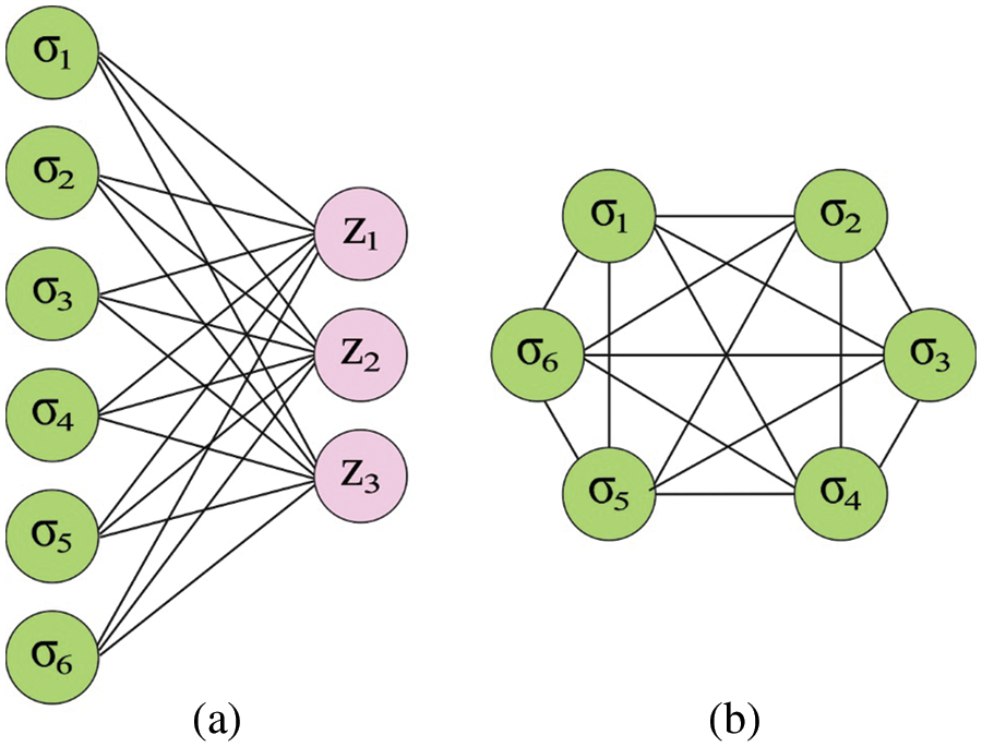
Figure 2: (a) Boltzmann machine (b) Hop field network

Ck=[c1k,c2k,…,cnk],

ωij={1a∑k=1K⁡cikcjk,i,j=1,2,…,n0,i=j(9)

whereas a indicates the adjusting ratio; take a=n. The process is given in the following:

Step 1: Initializing the network.

Step 2: The ith neuron is arbitrarily chosen in the networks.

Step 3: Evaluate the input value ui(t) for i-th neuron.

Step 4: Evaluate the output value νi(t+1) for i-th neuron. Now, the output of other neurons in the network remains same.

Step 5: to define either the network is stable or not: when it can be stable or meet the provided condition, it stops; or else, return to step 2.

Here, The steady state can be determined by (t+Δt)=ν(t), Δt>0.

2.3 Hyperparameter Optimization

In this work, the utilization of SMA assists in appropriately selecting the parameters involved in the DHNN approach [18]. The steps involved in SMA are given as follows.

Step 1: During this step, mathematics to the slime mold performance was created and subsequent rule was allocated for determining upgraded place in searching for food. The condition for this is dependent on r and p. It can be contraction mode of mold:

X(t+1)→={Xb(t)→+vb→⋅(W→⋅XA(t)→−XB(t)→)r<pvc→⋅X(t)→r≥p,(10)

In which vb→ signifies the parameter with range of --a and a, vc→ signifies the parameter that methods linearly nearby 0. ‘t’ implies the existing iteration, Xb→ signifies the place of all the particles from the region whereas odor is maximal, X→ refers to the mold place, X→A and X→B represents the arbitrarily chosen variables in the swarm, W→ signifies the measured of the weighted of masses. The maximal limit of p is given as follows:

p=tan⁡hS(i)−DFF|,(11)

whereas i∈1,2,…,n, S(i)= fitness of X→, DF= entire fitness in each step. The formula of v→ as follows:

vb→=[−a,a](12)

a=arctan⁡h(−(tmax−t)+1).(13)

The formula of W→ is listed as:

W(smellindex(i))→={1+r⋅log⁡(bF−S(i)bF−wF+1),condition1−r⋅log⁡(bF−S(i)bF−wF+1),others,(14)

SmellIndex=sort(S),(15)

whereas S(i) ranks first half of populations, r signifies the arbitrary value from the interval of zero and one, bF denotes the optimum fitness reached from the existing iterative procedure, wF refers to the worse fitness value reached from the iterative procedure, and Sort(s) function sort fitness value.

Step 2: The formula to upgrade the places of agents (that is, to wrap food) is provided as:

X∗→={rand⋅(UB−LB)+LB,rand<zXb(t)→+vb→⋅(W⋅XA(t)→−XB(t)→,r<p,vc→⋅X(t)→,r≥p(16)

In which, LB and UB indicate the searching limits, and rand and r signify the arbitrary values.

Step 3: Using the up gradation from the searching procedure, the value of vb→ vibrantly variations among --a and a, and vc→ differs amongst −1 and 1, and finally shrinks to 0. It can be recognized that ‘grabbling of food’.

3  Results and Discussion

In this section, the experimental validation of the SMADTL-CCDC model is tested using Warwick-QU dataset (www.warwick.ac.uk/fac/sci/dcs/research/tia/glascontest/download). It comprises 165 images with two class labels namely benign and malignant [19]. A few sample images of Colorectal Cancer are demonstrated in Fig. 3.

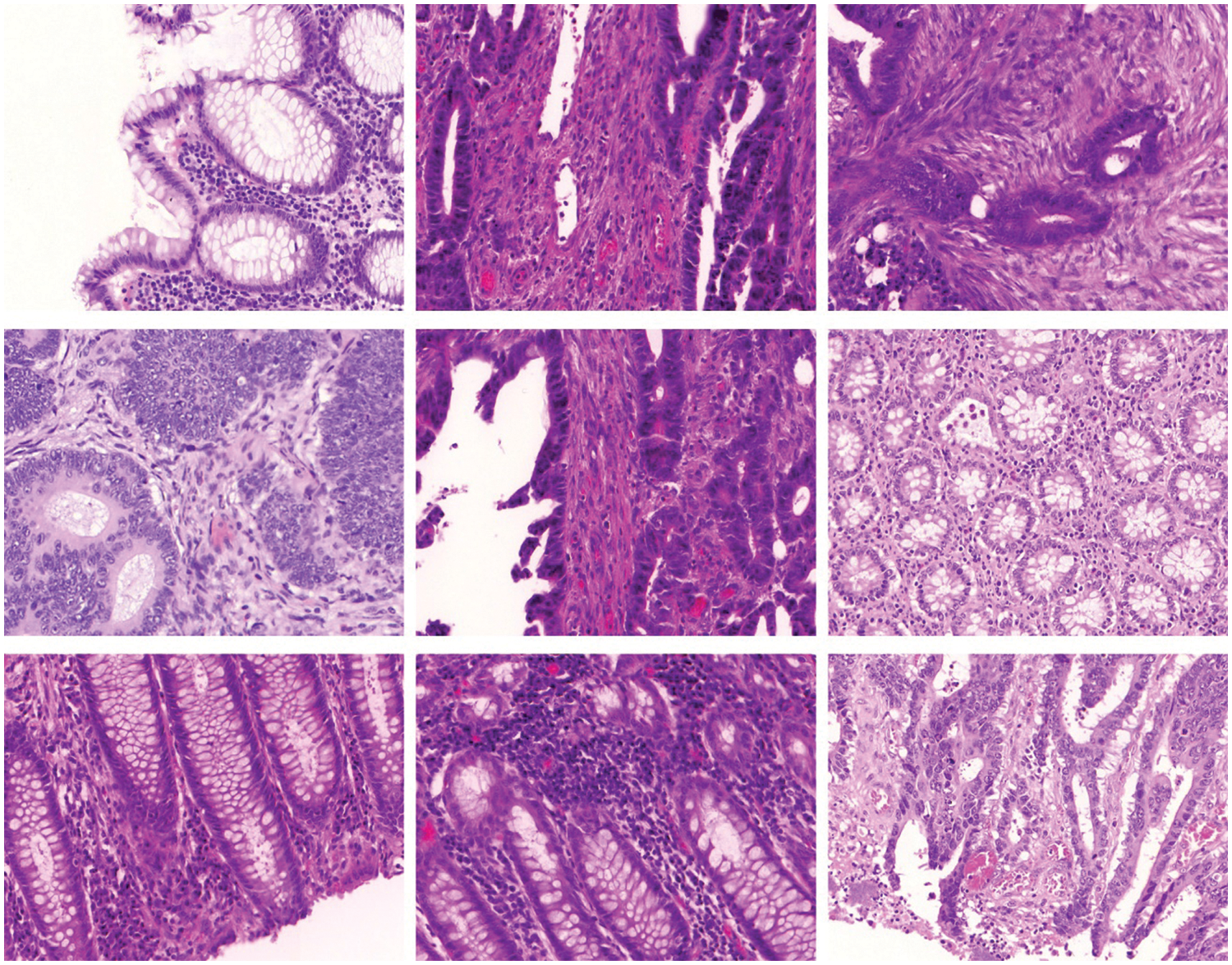
Figure 3: Sample images of colorectal cancer

Fig. 4 showcases the set of confusion matrices produced by the SMADTL-CCDC model on distinct sizes of training/testing (TR/TS) data. On 90% of TR data, the SMADTL-CCDC model has recognized 61 images into benign and 84 images into malignant. Also, on 80% of TR data, the SMADTL-CCDC approach has recognized 58 images into benign and 69 images into malignant. Besides, on 70% of TR data, the SMADTL-CCDC methodology has recognized 61 images into benign and 84 images into malignant.

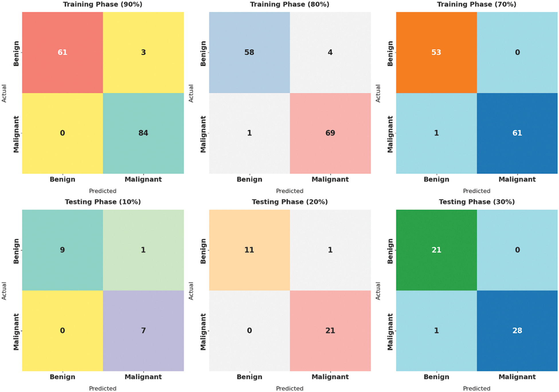
Figure 4: Confusion matrix of SMADTL-CCDC technique on distinct sizes of TR/TS data

Tab. 1 provides a detailed CRC classifier result of the SMADTL-CCDC model on TR/TS data of 90:10. The obtained values indicated that the SMADTL-CCDC model has accomplished improved performance in both cases. For instance, with 90% of TR data, the SMADTL-CCDC model has offered an average accuy, precn, recal, specy, and Fscore of 97.97%, 98.28%, 97.66%, 97.66%, and 97.92% respectively. At the same time, with 10% of TS data, the SMADTL-CCDC system has offered an average accuy, precn, recal, specy, and Fscore of 94.12%, 93.75%, 95%, 95%, and 94.04% correspondingly.

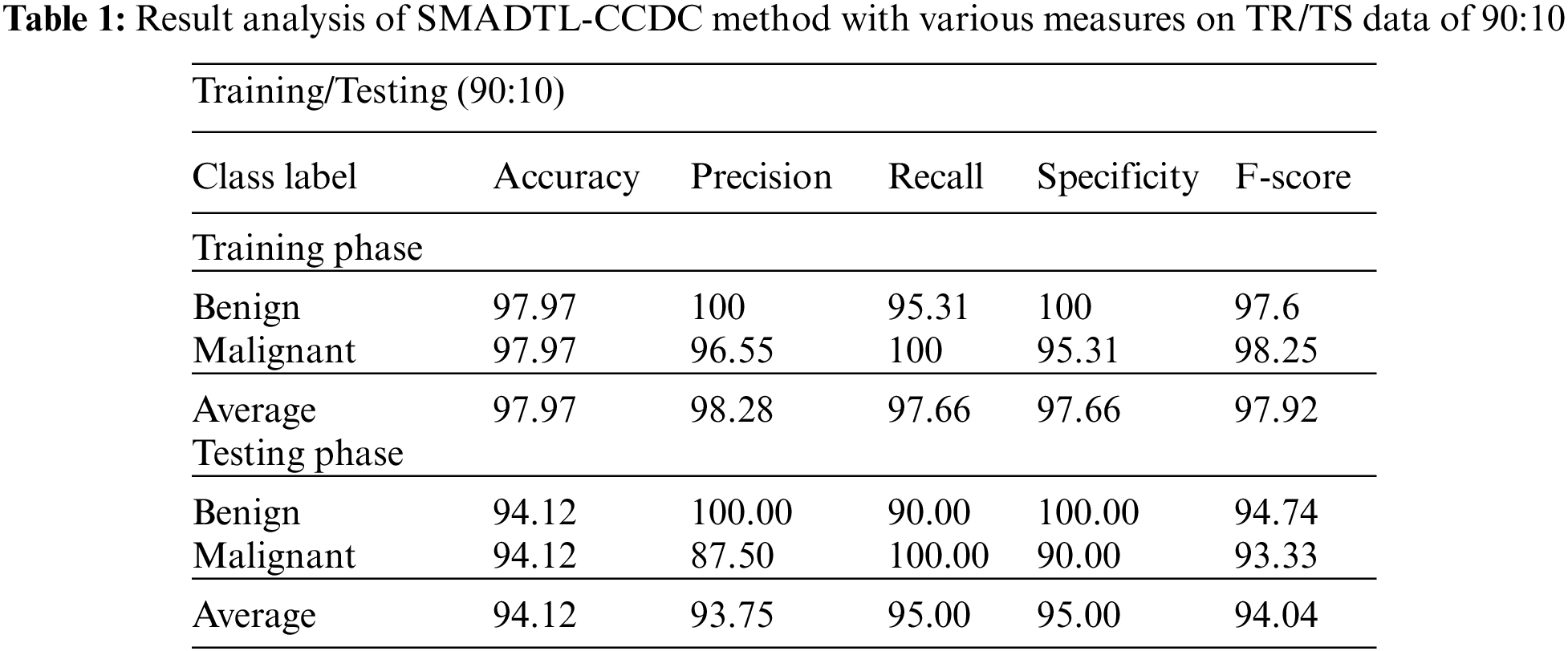
The training accuracy (TA) and validation accuracy (VA) attained by the SMADTL-CCDC model on TR/TS data of 90:10 is demonstrated in Fig. 5. The experimental outcomes implied that the ICSOA-DLPEC model has gained maximum values of TA and VA. In specific, the VA is seemed to be higher than TA.

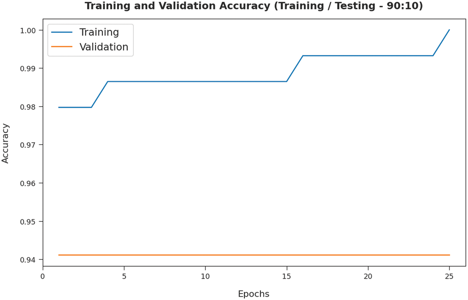
Figure 5: TA and VA analysis of SMADTL-CCDC model on TR/TS data of 90:10

The training loss (TL) and validation loss (VL) achieved by the SMADTL-CCDC model on TR/TS data of 90:10 is established in Fig. 6. The experimental outcomes inferred that the ICSOA-DLPEC model has accomplished least values of TL and VL. In specific, the VL is seemed to be lower than TL.

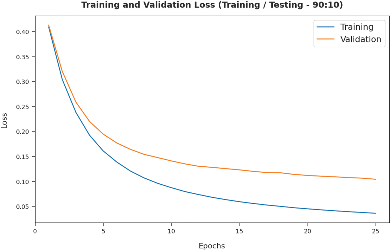
Figure 6: TL and VL analysis of SMADTL-CCDC model on TR/TS data of 90:10

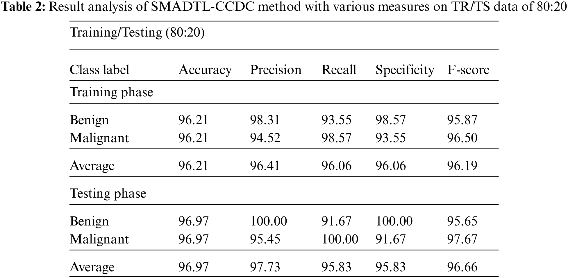
Tab. 2 offers a detailed CRC classifier result of the SMADTL-CCDC model on TR/TS data of 80:20. The obtained values referred that the SMADTL-CCDC approach has accomplished improved performance in both cases. For instance, with 80% of TR data, the SMADTL-CCDC model has offered an average accuy, precn, recal, specy, and Fscore of 96.21%, 96.41%, 96.06%, 96.06%, and 96.19% respectively. Eventually, with 20% of TS data, the SMADTL-CCDC methodology has offered an average accuy, precn, recal, specy, and Fscore of 96.97%, 97.73%, 95.83%, 95.83%, and 96.66% correspondingly.

The TA and VA attained by the SMADTL-CCDC model on TR/TS data of 80:20 are demonstrated in Fig. 7. The experimental outcomes implied that the ICSOA-DLPEC model has gained maximal values of TA and VA. In specific, the VA is seemed that higher than TA.

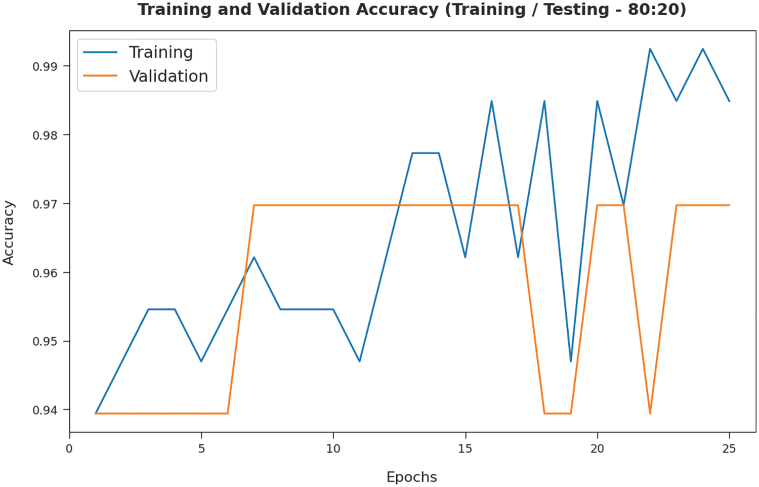
Figure 7: TA and VA analysis of SMADTL-CCDC model on TR/TS data of 80:20

The TL and VL achieved by the SMADTL-CCDC technique on TR/TS data of 80:20 are established in Fig. 8. The experimental outcomes inferred that the ICSOA-DLPEC model has accomplished least values of TL and VL. In specific, the VL has appeared that lower than TL.

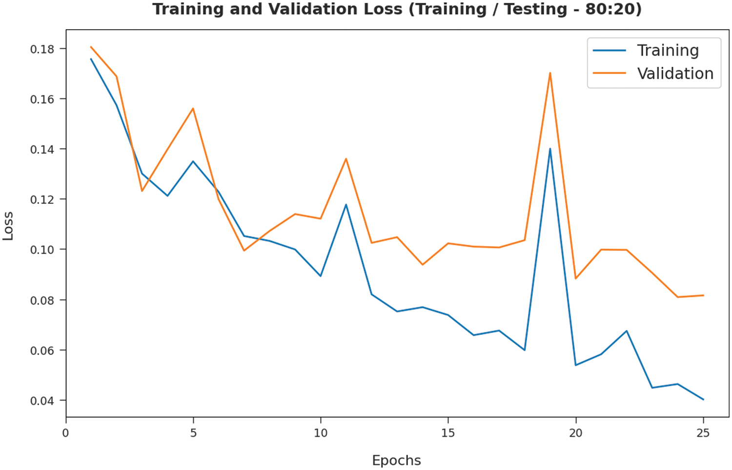
Figure 8: TL and VL analysis of SMADTL-CCDC model on TR/TS data of 80:20

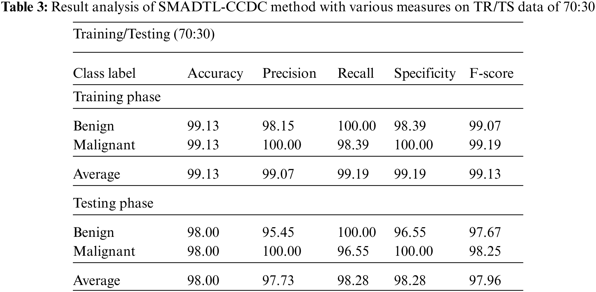
Tab. 3 gives a detailed CRC classifier result of the SMADTL-CCDC system on TR/TS data of 70:30. The obtained values indicated that the SMADTL-CCDC approach has accomplished enhanced performance in both cases. For instance, with 70% of TR data, the SMADTL-CCDC algorithm has offered an average accuy, precn, recal, specy, and Fscore of 99.13%, 99.07%, 99.19%, 99.19%, and 99.13% respectively. In addition, with 30% of TS data, the SMADTL-CCDC system has offered an average accuy, precn, recal, specy, and Fscore of 98%, 97.73%, 98.28%, 98.28%, and 97.96% correspondingly.

The TA and VA attained by the SMADTL-CCDC algorithm on TR/TS data of 70:30 are demonstrated in Fig. 9. The experimental outcomes implied that the ICSOA-DLPEC model has gained maximum values of TA and VA. In specific, the VA is appeared to be higher than TA.

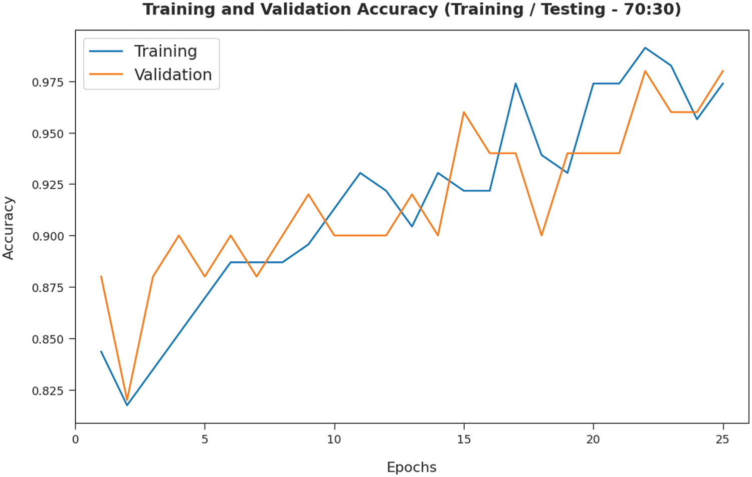
Figure 9: TA and VA analysis of SMADTL-CCDC model on TR/TS data of 70:30

The TL and VL achieved by the SMADTL-CCDC model on TR/TS data of 70:30 are established in Fig. 10. The experimental outcomes inferred that the ICSOA-DLPEC technique has accomplished least values of TL and VL. In specific, the VL is seemed to be lower than TL.

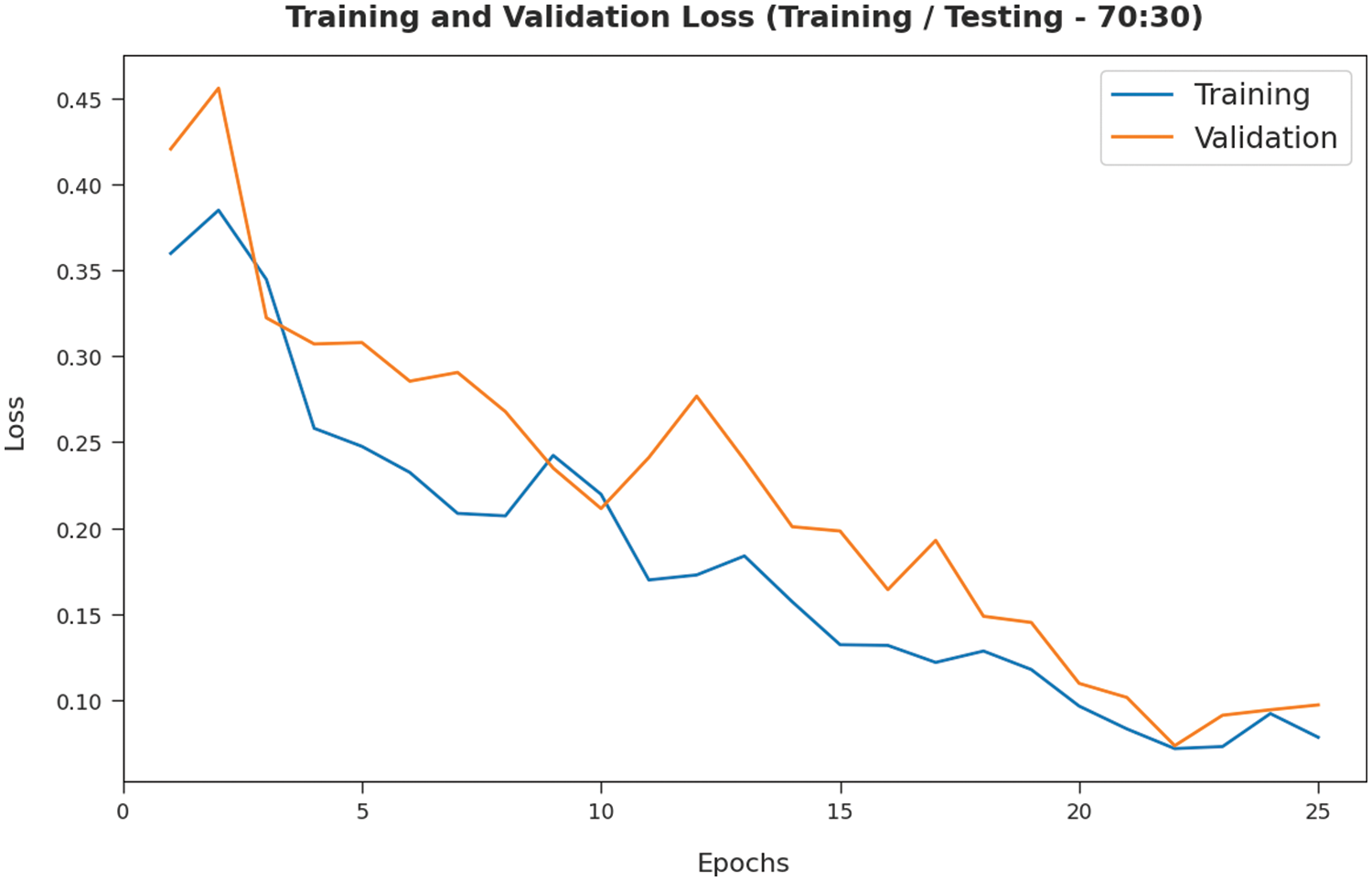
Figure 10: TL and VL analysis of SMADTL-CCDC model on TR/TS data of 70:30

Fig. 11 provides a comparative sensy examination of the SMADTL-CCDC model with existing models [20–23]. The figure reported that the ResNet-18 (60-40), ResNet-50 (60-40), and DL-CP models have attained lower sensy values of 66.29%, 61.69%, and 70.93% respectively. In addition, the ResNet-18 (80-20), ResNet-50 (75-25), ResNet-50 (80-20), and DL-SC Models have obtained slightly increased sensy values of 84.67%, 90.78%, 94.79%, and 84.80% respectively. Though the ResNet-18 (75-25) model has accomplished reasonably sensy of 98.26%, the SMADTL-CCDC model has resulted in superior sensy of 98.28%.

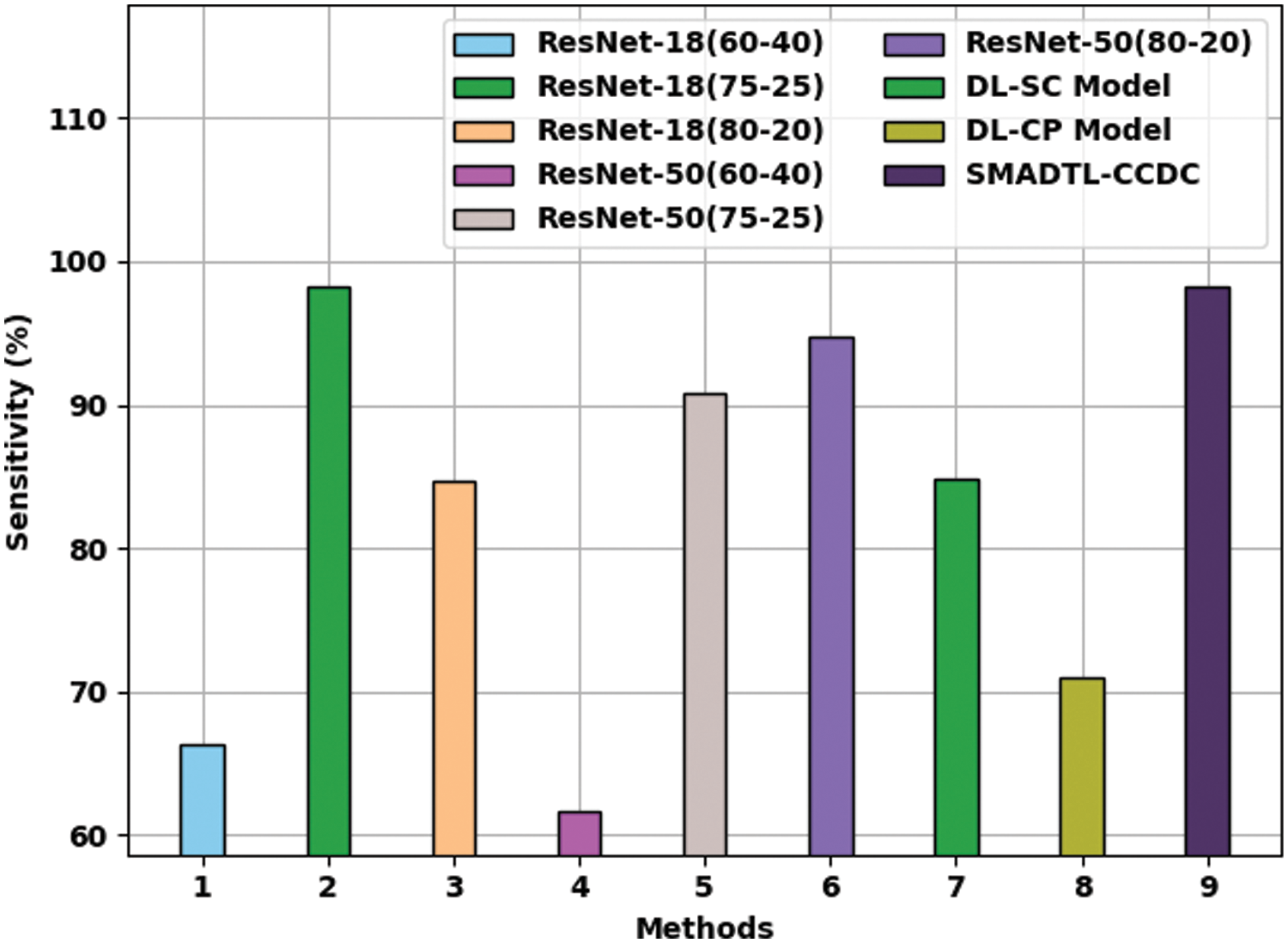
Figure 11: Sensy analysis of SMADTL-CCDC approach with recent methodologies

Fig. 12 offers a comparative specy analysis of the SMADTL-CCDC model with existing models. The figure exposed that the ResNet-18 (75.25), DL-CP, and DL-SC models have attained lower specy values of 65.30%, 73.04%, and 82.82% correspondingly. Also, the ResNet-18 (60-40), ResNet-50 (80-20), ResNet-18 (75-25), and ResNet-18 (80-20) Models have obtained somewhat improved specy values of 84.71%, 85.42%, 89.10%, and 89.11% correspondingly. But the ResNet-50 (60-40) approach has accomplished reasonably specy of 94.35%, the SMADTL-CCDC model has resulted in superior specy of 98.28%.

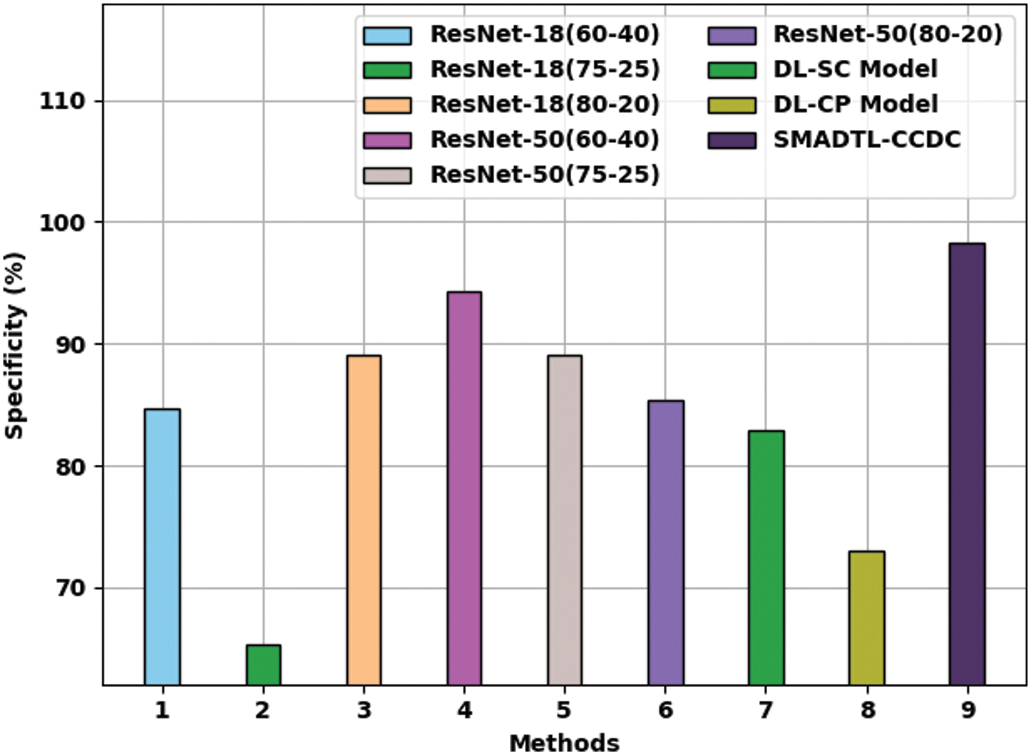
Figure 12: Specy analysis of SMADTL-CCDC approach with recent methodologies

Fig. 13 gives a comparative accy examination of the SMADTL-CCDC model with existing models. The figure reported that the DL-CP, ResNet-18 (60-40), and ResNet-50 (60-40) approaches have attained lower accy values of 72.28%, 74.76%, and 7.23% correspondingly. Morover, the ResNet-18 (75-25), DL-SC, ResNet-18 (80-20), and ResNet-50 (75-25) Models have obtained slightly increased accy values of 83.19%, 83.47%, 87.56%, and 89.70% correspondingly. At last, the ResNet-50 (80-20) algorithm has accomplished reasonably accy of 90.25%, the SMADTL-CCDC approach has resulted in higher accy of 98%.

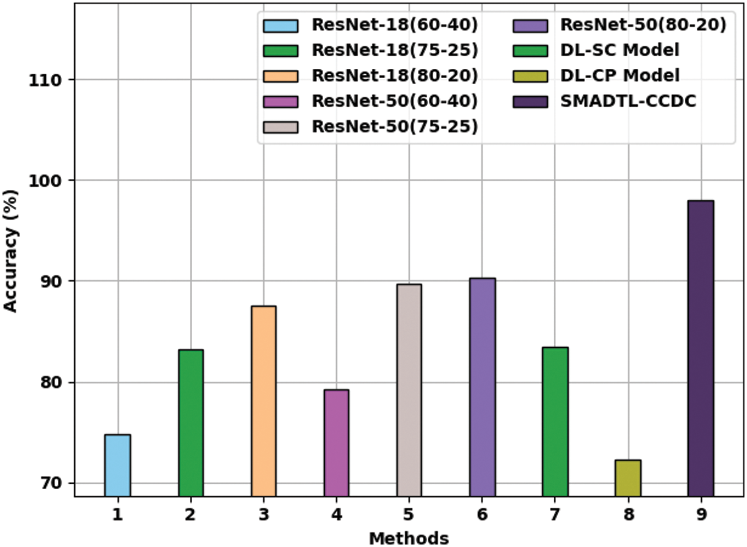
Figure 13: Accy analysis of SMADTL-CCDC approach with recent methodologies

From the detailed results and discussion, it can be evident that the SMADTL-CCDC model has gained maximum performance over the other methods.

4  Conclusion

In this study, a new SMADTL-CCDC model has been developed to appropriately recognize the occurrence of CRC. The SMADTL-CCDC model originally undergoes pre-processing to improve the input image quality. Followed by, a dense-EfficientNet approach was employed to extract feature vectors in the pre-processed images. Moreover, SMA with DHNN technique was executed for the recognition and classification of CRC. The utilization of SMA assists in appropriately selecting the parameters contained in the DHNN approach. A wide range of experiments is applied to benchmark datasets to assess the classification performance. A comprehensive comparative study highlighted the better performance of the SMADTL-CDC technique on the recent approaches. In future, hybrid DL models can be employed to perform classification processes.

Funding Statement: This work was funded by the Deanship of Scientific Research (DSR) at King AbdulAziz University (KAU), Jeddah, Saudi Arabia, under grant no. (DF-497-141-1441). The authors, therefore, gratefully acknowledge DSR for technical and financial support.

Conflicts of Interest: The authors declare that they have no conflicts of interest to report regarding the present study.

References

1. D. Bychkov, N. Linder, R. Turkki, S. Nordling, P. E. Kovanen et al., “Deep learning based tissue analysis predicts outcome in colorectal cancer,” Scientific Reports, vol. 8, no. 1, pp. 3395, 2018. [Google Scholar]
2. O.-J. Skrede, S. D. Raedt, A. Kleppe, T. Shveem, K. Liestøl et al., “Deep learning for prediction of colorectal cancer outcome: A discovery and validation study,” The Lancet, vol. 395, no. 10221, pp. 350–360, 2020. [Google Scholar]
3. J. N. Kather, C. A. Weis, F. Bianconi, S. M. Melchers, L. R. Schad et al., “Multi-class texture analysis in colorectal cancer histology,” Scientific Reports, vol. 6, no. 1, pp. 1–11, 2016. [Google Scholar]
4. J. Xu, X. Luo, G. Wang, H. Gilmore and A. Madabhushi, “A deep convolutional neural network for segmenting and classifying epithelial and stromal regions in histopathological images,” Neurocomputing, vol. 191, no. 11, pp. 214–223, 2016. [Google Scholar]
5. W. Wang, Y. T. Li, T. Zou, X. Wang, J. Y. You et al., “A novel image classification approach via Dense-MobileNet models,” Mobile Information Systems, vol. 2020, pp. 1–8, 2020. [Google Scholar]
6. S. R. Zhou, J. P. Yin and J. M. Zhang, “Local binary pattern (LBP) and local phase quantization (LBQ) based on Gabor filter for face representation,” Neurocomputing, vol. 116, no. 6 (June), pp. 260–264, 2013. [Google Scholar]
7. Y. Song, D. Zhang, Q. Tang, S. Tang and K. Yang, “Local and nonlocal constraints for compressed sensing video and multi-view image recovery,” Neurocomputing, vol. 406, no. 2, pp. 34–48, 2020. [Google Scholar]
8. D. Zhang, S. Wang, F. Li, S. Tian, J. Wang et al., “An efficient ECG denoising method based on empirical mode decomposition, sample entropy, and improved threshold function,” Wireless Communications and Mobile Computing, vol. 2020, no. 2, pp. 1–11, 2020. [Google Scholar]
9. F. Li, C. Ou, Y. Gui and L. Xiang, “Instant edit propagation on images based on bilateral grid,” Computers, Materials & Continua, vol. 61, no. 2, pp. 643–656, 2019. [Google Scholar]
10. Y. Song, Y. Zeng, X. Y. Li, B. Y. Cai and G. B. Yang, “Fast CU size decision and mode decision algorithm for intra prediction in HEVC,” Multimedia Tools and Applications, vol. 76, no. 2, pp. 2001–2017, 2017. [Google Scholar]
11. N. Dif and Z. Elberrichi, “A new deep learning model selection method for colorectal cancer classification,” International Journal of Swarm Intelligence Research, vol. 11, no. 3, pp. 72–88, 2020. [Google Scholar]
12. D. Sarwinda, R. H. Paradisa, A. Bustamam and P. Anggia, “Deep learning in image classification using residual network (resnet) variants for detection of colorectal cancer,” Procedia Computer Science, vol. 179, no. 3, pp. 423–431, 2021. [Google Scholar]
13. M. Mulenga, S. A. Kareem, A. Q. M. Sabri, M. Seera, S. Govind et al., “Feature extension of gut microbiome data for deep neural network-based colorectal cancer classification,” IEEE Access, vol. 9, pp. 23565–23578, 2021. [Google Scholar]
14. C. Ho, Z. Zhao, X. F. Chen, J. Sauer, S. A. Saraf et al., “A promising deep learning-assistive algorithm for histopathological screening of colorectal cancer,” Scientific Reports, vol. 12, no. 1, pp. 2222, 2022. [Google Scholar]
15. M. J. Tsai and Y. H. Tao, “Deep learning techniques for the classification of colorectal cancer tissue,” Electronics, vol. 10, no. 14, pp. 1662, 2021. [Google Scholar]
16. D. R. Nayak, N. Padhy, P. K. Mallick, M. Zymbler and S. Kumar, “Brain tumor classification using dense efficient-net,” Axioms, vol. 11, no. 1, pp. 34, 2022. [Google Scholar]
17. C. Hu, Y. Ma and T. Chen, “Application on online process learning evaluation based on optimal discrete hopfield neural network and entropy weight topsis method,” Complexity, vol. 2021, pp. 1–9, 2021. [Google Scholar]
18. D. Dhawale, V. K. Kamboj and P. Anand, “An effective solution to numerical and multi-disciplinary design optimization problems using chaotic slime mold algorithm,” Engineering with Computers, 2021. https://doi.org/10.1007/s00366-021-01409-4. [Google Scholar]
19. K. Sirinukunwattana, D. R. J. Snead and N. M. Rajpoot, “A stochastic polygons model for glandular structures in colon histology images,” IEEE Transactions on Medical Imaging, vol. 34, no. 11, pp. 2366–2378, 2015. [Google Scholar]
20. K. Sirinukunwattana, S. E. A. Raza, Y. W. Tsang, D. R. J. Snead, I. A. Cree et al., “Locality sensitive deep learning for detection and classification of nuclei in routine colon cancer histology images,” IEEE Transactions on Medical Imaging, vol. 35, no. 5, pp. 1196–1206, 2016. [Google Scholar]
21. M. Ragab, A. Albukhari, J. Alyami and R. F. Mansour, “Ensemble deep-learning-enabled clinical decision support system for breast cancer diagnosis and classification on ultrasound images,” Biology, vol. 11, no. 3, pp. 439, 2022. [Google Scholar]
22. J. E. Gutierrez, R. F. Mansour, K. Beleño, J. J. Cabas, M. Pérez et al., “Automated deep learning empowered breast cancer diagnosis using biomedical mammogram images,” Computers, Materials & Continua, vol. 71, no. 3, pp. 4221–4235, 2022. [Google Scholar]
23. S. K. Lakshmanaprabu, S. N. Mohanty, K. Shankar, N. Arunkumar and G. Ramirez, “Optimal deep learning model for classification of lung cancer on CT images,” Future Generation Computer Systems, vol. 92, no. 1, pp. 374–382, 2019. [Google Scholar]
Cite This Article
Copyright © 2023 The Author(s). Published by Tech Science Press.
This work is licensed under a Creative Commons Attribution 4.0 International License , which permits unrestricted use, distribution, and reproduction in any medium, provided the original work is properly cited.
Downloads
Citation Tools