
 Submit a Paper
 Propose a Special lssue
 Open Access
ARTICLE

Vibration of a Two-Layer “Metal+PZT” Plate Contacting with Viscous Fluid
1 Department of Mechanical Engineering, Kirsehir Ahi Evran University, Kirsehir, 40100, Turkey
2 Department of Mechanical Engineering, Yildiz Technical University, Yildiz Campus, Istanbul, 34349, Turkey
3 Institute of Mathematics and Mechanics of the National Academy of Sciences of Azerbaijan, Baku, 37041, Azerbaijan
* Corresponding Author: Zeynep Ekicioglu Kuzeci. Email:
Computers, Materials & Continua 2023, 74(2), 4337-4362. https://doi.org/10.32604/cmc.2023.033446
Received 16 June 2022; Accepted 02 September 2022; Issue published 31 October 2022
 View Full Text
 Download PDF
Abstract
The present work investigates the mechanically forced vibration of the hydro-elasto-piezoelectric system consisting of a two-layer plate “elastic+PZT”, a compressible viscous fluid, and a rigid wall. It is assumed that the PZT (piezoelectric) layer of the plate is in contact with the fluid and time-harmonic linear forces act on the free surface of the elastic-metallic layer. This study is valuable because it considers for the first time the mechanical vibration of the metal+piezoelectric bilayer plate in contact with a fluid. It is also the first time that the influence of the volumetric concentration of the constituents on the vibration of the hydro-elasto-piezoelectric system is studied. Another value of the present work is the use of the exact equations and relations of elasto-electrodynamics for elastic and piezoelectric materials to describe the motion of the plate layers within the framework of the piecewise homogeneous body model and the use of the linearized Navier-Stokes equations to describe the flow of the compressible viscous fluid. The plane-strain state in the plate and the plane flow in the fluid take place. For the solution of the corresponding boundary-value problem, the Fourier transform is used with respect to the spatial coordinate on the axis along the laying direction of the plate. The analytical expressions of the Fourier transform of all the sought values of each component of the system are determined. The origins of the searched values are determined numerically, after which numerical results on the stress on the fluid and plate interface planes are presented and discussed. These results are obtained for the case where PZT-2 is chosen as the piezoelectric material, steel and aluminum as the elastic metal materials, and Glycerin as the fluid. Analysis of these results allows conclusions to be drawn about the character of the problem parameters on the frequency response of the interfacial stress. In particular, it was found that after a certain value of the vibration frequency, the presence of the metal layer in the two-layer plate led to an increase in the absolute values of the above interfacial stress.Keywords
In the classical sense, the study of the dynamics of a piecewise homogeneous acoustic medium, such as “plate+fluid” systems in the cases where the plate is made of conventional metal or polymer materials, is necessary for various fields of modern industry, e.g., fluid transport, geophysical investigations, biomedical device construction, submarine construction and sound insulation. The results of these studies provide a theoretical basis for understanding the acoustic phenomena occurring in the piecewise homogeneous acoustic medium. Consequently, these results provide opportunities for the control and management of these phenomena.
In modern literature, the work of Lamb [1], completed a hundred years ago, is considered the beginning of these studies. Since then, a lot of further research has been done. For a detailed review, as well as some recent results, see the works of Amabili [2], Akbarov [3,4], Akbarov et al. [5–7], Guz [8], Guz et al. [9], Paimushin et al. [10], Paimushin et al. [11], Shuaib et al. [12], Sorokin et al. [13], Zamanov et al. [14] and many others listed therein.
Note that these investigations can be classified according to various aspects, such as the theories applied to describe the motion of the plate (approximate plate theories, which are described, for example in [1,2,10–12] and many other theories discussed in the work of Akbarov [3]); the exact equations of elastodynamics discussed for example in [5–9]; and modeling of the plate material as elastic, for example, in the work of Akbarov et al. [6] and many other works listed therein, or viscoelastic, for example, in the works [7,14]. Moreover, these works can be classified according to the type of dynamic problems considered (wave dispersion, free vibration, and forced vibration), the modeling of the fluid (inviscid fluid, viscous fluid, compressible and incompressible fluid), and so on.
The aforementioned works serve not only their direct purpose but also provide the theoretical basis for the study of the corresponding problems related to the cases in which the plate material is intelligent, such as piezoelectric or piezomagnetic. It should be noted that the results of such investigations have great importance for energy harvesting procedures (see, for example, references [15–18] and others listed therein), and in hydroacoustic transducers that receive (or generate) acoustic waves (see, for example references [19–21] and others listed therein).
Nevertheless, there has not been enough fundamental theoretical research in this field, to which the present research is dedicated, in particular, to the mechanical forced vibration of the hydro-piezoelectric system consisting of a two-layer “metal+PZT” plate, a compressible viscous fluid, and a rigid wall. The research presented here is carried out in the framework of the piecewise-homogeneous body model using the exact equations and relations of elastodynamics and electrodynamics in the plane-strain state to describe the motion of the “metal+piezoelectric” plate and using the linearized Navier-Stokes equations for the plane flow of the compressible viscous fluid.
To show the relevance and importance of the present work, let us consider a brief review of related research and begin with the work of Belkourchia et al. [16], in which the algorithm is developed for the numerical solution of the problem related to determination of the pressure exerted by ocean motion waves on a vertical cantilever beam with piezoelectric patches where the motion of the cantilever is described within the framework of the Euler-Bernoulli beam theory, but the flow of the fluid is described by the Navier-Stokes equations for the incompressible viscous fluid. This does not take into account the piezoelectricity of the patches, and it is assumed that determination of the fluid pressures acting on the left and right sides of the cantilever allows for calculation of the electric potentials occurring in the piezoelectric patches. In this way, extraction of the energy originating from the fluid motion can be controlled. The work of Akaydin et al. [22] and others listed therein also use a similar approach, but the material of the cantilever is taken as a piezoelectric one. In addition, the Euler-Bernoulli beam model is used in many studies listed in the conference book [23] on this topic.
The piezoelectric composite cantilever beam model is also used in the work of He et al. [24] to determine the optimal thickness of the PZT layer in the piezoelectric energy harvesters (PEH) to obtain the maximum electrical energy under static mechanical and external electrical excitation. FEM (finite element method) is used in the framework of the exact relations of linear piezoelectricity to obtain concrete numerical results on the influence of the volume fraction of the PZT material on electrical energy. However, the approach developed in the work of He et al. [24] is not only related to the cantilever beam model, but also to more general PEH models. In the work of Chen et al. [25], the effect of geometric nonlinearity and flexoelectricity on the uniform and bimorph PEH under harmonic mechanical excitation is analyzed. The model of a cantilever beam is also considered and the motion of these beams is described in the framework of the Euler-Bernoulli beam theory. Hamilton’s principle is used to obtain the equations of motion and these equations are solved using Galerkin’s method.
In contrast to the aforementioned work, the work by Amini et al. [15] attempts to use the three-dimensional exact equations of motion of elasto-electrodynamics to describe the motion of the piezoelectric cantilever. There are also many studies of the dynamics of intelligent systems that relate to linear and nonlinear vibrations, and dispersion of the waves propagating therein. Examples of such recent investigations can be found in the papers [26–28] and many others presented therein. Let us consider briefly the subjects of these works and begin with the work of Jiang et al. [26] which presents a nonlinear piezoelectric energy harvester with two degrees of freedom to improve the efficiency of energy harvesting at low frequencies. An L-shaped piezoelectric cantilever beam is considered, and this beam is assumed to be excited by nonlinear attractive forces of magnets attached to the end of the cantilever and to the base. The dynamic equation for the PZT beam is derived from the magnetic attraction force mentioned above. Under the harmonic excitation, this equation is solved numerically and the range of change of the problem parameters is determined, which improves the harvesting properties of the system.
The work of Nie et al. [27] investigates the dispersion of the propagating Rayleigh-type waves in the system consisting of the piezoelectric layer and a semi-infinite dielectric substrate. The material of the piezoelectric layer is assumed to be a cubic crystal and the contact conditions on the interface of the constituents of the system are assumed to be mechanically perfect but electrically imperfect. Dispersion relations for electrically open or short-circuited boundary conditions are obtained and analyzed.
The paper by Qiao et al. [28] presents a theoretical analysis of the technology for vibration control of wind turbine blades by using piezoelectric smart structures. Since the design of the blade structure made of piezoelectric material is similar to a shallow shell structure, the equations of motion are derived based on the theory of piezoelectric laminated shallow shells. Based on the solution of these equations, it is found that the blade vibration under wind load can be reduced by applying control voltage.
In all the above works dealing with hydro-piezoelectric systems, the fluid flow is described in the framework of the incompressible viscous or inviscid Newtonian fluid model using the linear Navier-Stokes equations. Moreover, in these works, the motion (or vibration) of the piezoelectric cantilevers is considered with finite sizes, so such a model cannot discover the local electromechanical and hydro-electromechanical coupling effects without the influence of the boundary conditions. Such an effect related to the subject of the present work can be discovered in the framework of infinite two-layer “metal+piezoelectric” plate and fluid systems.
Note also that the above work does not investigate how the electromechanical coupling effect of the piezoelectric material can affect the pressure at the interface between the fluid and the plate. Since the energy generation in the energy harvesting piezoelectric systems comes from this pressure, the above coupling effects must be considered in theoretical studies.
In order to address the above issues, Ekicioglu Kuzeci [29] carried out some investigations in this field and studied the mechanically forced vibration of the hydro-piezoelectric system consisting of the infinite piezoelectric plate and the compressible (barotropic) Newtonian viscous fluid with finite depth. The flow of the fluid is described by the linearized Navier-Stokes equations, while the motion of the plate is described by the exact equations of the theory of electroelasticity for piezoelectric materials.
In the present paper, an attempt is made to develop these investigations for the system consisting of a two-layer “metal+piezoelectric” plate, a compressible viscous fluid, and a rigid wall. The motion of the plate is described within the piecewise-homogeneous body model using the exact equations of elasto-and electrodynamics for piezoelectric materials, and the flow of the fluid is described using the linearized Navier-Stokes equations for a compressible viscous fluid.
The present work can also be considered as further development of the second author’s work from the last decade dealing with the forced vibration of single-layer purely elastic or viscoelastic plates in contact with a compressible viscous fluid (see, for example, the works [5–7]). A review of these works can be found in the paper by Akbarov [3]. Note that a number of studies have also been carried out on the problem of the dispersion of waves in hydro-elastic systems consisting of a single-layer purely elastic plate and a compressible fluid. Their data and considerations are contained in the works of Guz et al. [9] and Guz [8].
Thus, it is clear that the investigations on the subject of the present work were carried out for the case where the plate is single-layered. Thus, the main difference of the present work from the previous related works of the second author and his collaborators, as well as from the investigations described in the works [8,9], is the two-layer nature of the plate and the piezoelectricity of the material of one of the layers.
Note that in the formulation of the problem studied in this paper, we use the linearized Navier-Stokes equations obtained from the corresponding nonlinear Navier-Stokes equations for compressible barotropic viscous fluids. Linearization is one of the methods for solving nonlinear problems. Many other methods for solving nonlinear physical-mechanical problems have been developed in recent years. We briefly review some here and begin with the work of Mahdy et al. [30], in which the reduced differential transform method is used to solve the nonlinear fractional model tumor-immune. The same method is also used in the work of Gepreel et al. [31] to solve nonlinear biomathematical problems related to the spread of viruses in a computer network and to the problem of susceptible infected-recovered (SIR) childhood diseases.
Moreover, in a series of studies by Bazighifan et al. [32], Santra et al. [33], Bazighifan et al. [34], Bazighifan et al. [35], Moaaz et al. [36], and many others listed therein, the nonlinear differential equations of even order are studied with p-Laplacian-like operators, the results of which shed light on the solution of the corresponding nonlinear problems in continuum mechanics. In the work of Bazighifan [37], a new type of oscillation criterion is established for a neutral differential equation of even order. In the work of Santra et al. [33], sufficient conditions for oscillation of all solutions of a second-order functional differential equation are found. New results on the oscillation of solutions of a class of advanced even-order differential equations with p-Laplacian-like operators are obtained in the work of Bazighifan et al. [35]. The asymptotic peculiarities for a class of fourth order neutral differential equations are studied in the work of Bazighifan et al. [34]. New sufficient conditions for the oscillation of fourth order neutral differential equations are found in the work of Moaaz et al. [36]. The work of Moaaz et al. [38] deals with the oscillation of a class of third order nonlinear delay differential equations with mean term and a new description of the oscillation of third order linear differential equation without damping is proposed. Finally, in the work of Moaaz et al. [39], the general class of differential equations is considered (the particular cases of which have been studied previously by the authors of the related works mentioned above) and the corresponding general theorems for the asymptotic behavior of the solution of these equations are established.
In this context, since the present study refers to coupling field problems, we refer to the recent studies of Mahdy et al. [40], Mohammed et al. [41], Khamis et al. [42], Mahdy et al. [43] and many others within these works, which also refer to coupling field problems. The novel model of photothermoelasticity theory is studied in the work [40]. A novel mathematical model is proposed and applied in [41] to study the micro stretch properties of an elastic semiconductor medium. In papers [42,43], novel mathematical models are developed for the piezoelectric elastic semiconductor medium and photothermoelasticity theory, respectively.
The remainder of this paper is organized as follows. The mathematical formulation of the problem, the equation of motion of the metal/PZT plate and the equations of flow, as well as the corresponding boundary, contact, and compatibility conditions are given in Section 2. The solution method for the formulated boundary value problem and the algorithm for obtaining the numerical results are explained in Section 3. The numerical results are presented and discussed in Section 4, and finally, the results are summarized in Section 5.
2 Formulation of the Problem and Governing Field Equations and Relations
We consider the hydro-elastic-piezoelectric system shown in Fig. 1, which consists of a two-layer “metal+piezoelectric” plate, a compressible barotropic viscous fluid, and a rigid wall that limits the fluid depth. Associate the Cartesian coordinate system
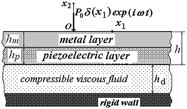
Figure 1: The sketch of the hydro-elastic-piezoelectric system
In this framework, it is required to determine the mechanical and electrical fields in the above hydro-elastic-piezoelectric system by using the appropriate exact field equations and relations. For this purpose, we write these field equations and relations for each component of the system, using the upper indices (m) and (p) to indicate the affiliation of the quantities to the metallic and piezoelectric layers, respectively. According to the monograph by Yang [44], the equations of motion for the metal and piezoelectric layers can be written as follows:
where
In addition, the following relations are:
Mechanical relations for the metal layer material:
Electro–mechanical relations for the piezoelectric layer material when it is polarized along the
In (2) and (3),
In Eqs. (1)–(4),
This completes the field equations and relations describing the motion of the two-layer “metal+piezoelectric” plate. Now we try to write the field equations and relations for the compressible (barotropic) viscous fluid flow. According to the monograph of Guz [8], the linearized equations of the fluid flow for the considered case can be represented as follows:
where the first equation of (5) is the continuity equation, but the last two equations of (5) are the linearized Navier-Stokes equations, which must be provided with the linearized rheological relations and the linearized equation of state given below:
where
In (5)–(7), the following notation is used:
According to the monograph by Guz [8], we also add the following representations for the velocities
where the potentials
where
Now we try to formulate the corresponding boundary conditions at the
The boundary conditions on the upper face plane of the plate are:
where
Perfect contact conditions on the plane between the metal and piezoelectric layers are:
Compatibility conditions on the interface plane between the fluid and plate are:
The impermeability conditions on the rigid wall are:
We also add the boundary conditions on the planes
This completes the formulation of the problems investigated in the present paper.
The presence of piezoelectric components in composite materials complicates the analytical solution of the corresponding problems. Therefore, it sometimes seems necessary to apply numerical methods, as in the works of Aylikci et al. [45], Ray et al. [46] and in many other works listed therein, to solve the corresponding problems. However, in the present case, the exponential Fourier transform is successfully used to solve the corresponding boundary value problem in obtaining an analytical expression for the transforms of the sought values whose originals are found numerically.
According to the definition of the time-harmonic oscillation, let us represent all the sought values of the considered problem as
According to which, the amplitudes can be presented as follows:
Now, we consider separately the determination of the Fourier transforms of the quantities related to the metal and piezoelectric layers of the plate and related to the fluid.
3.1 Determination of the Fourier Transforms of the Quantities Related to the Elastic-Metal Plate
Substituting the expressions related to the metal layer given in (16) into the Eqs. (2) and (4), we obtain the following equations of motion for the metal layer with respect to the displacement terms:
where
and in (17) under
we can write the solution of the Eq. (17) as follows:
where
Using the relations (2), (4) and (20), we obtain the expressions for the Fourier transforms of the stresses
3.2 Determination of the Fourier Transforms of the Quantities Related to the Piezoelectric Layer
Substituting the expressions in (16) into the foregoing equations and relations in (1), (3), and (4) and doing the corresponding mathematical manipulations, we obtain the following system of the ordinary differential equations for
where
We recall that in Eq. (22) under
In (24), the lower index
Thus, substituting the particular solutions in (24) into the system of equations in (22) and employing the usual procedures, we obtain the following system of homogeneous linear algebraic equations with respect to the unknown constants
According to the requirement of the existence of the non-trivial solution of the system of equations in (25), we equate to zero the determinant of the coefficient matrices of this system and we obtain the following bi-cubic equation for determination of the unknown constant b.
where
In (27), the notation given below is used.
We employ Vieta’s trigonometric formula for cubic equations in order to find the roots of the Eq. (26), according to which, in the first step, the values of the following expressions must be calculated.
In the next step, the values of the expression in (30) are calculated.
According to the sign of S, the cases are distinguished. So if
However, if
In this way, we determine the roots of the characteristic Eq. (26) and we can write the six roots of the bi-cubic equation as follows:
According to the expressions in (24) and to the solution technique used, the general solution to the system of ordinary differential equations in (22) is:
where
Substituting the expressions in (34) into the Fourier transform of the relations in (3) and (4), we obtain the following expressions for the stresses and electrical displacement which enter into the boundary, contact and compatibility conditions:
Thus, the expressions of the Fourier transforms of the values related to the piezoelectric plate are completely determined.
3.3 Determination of the Fourier Transforms of the Quantities Related to the Fluid
To determine the Fourier transforms of the quantities related to the fluid flow, first we consider determination of
Substituting the expressions in (37) into the Fourier transform of the equations in (9), after some mathematical manipulations, the following equations are obtained for the functions
where
Note that the dimensionless numbers
Thus, according to the well-known solution technique of ordinary differential equations, the solution to the equations in (38) can be presented as follows:
where
Using the expressions in (37), (40), (8), (7), and (6), the following expressions are obtained for the quantities related to the fluid flow:
where
Finally, we obtain a system of 14 linear algebraic equations which contains 14 unknown constants by substituting the expressions in (34), (36) and (42) into the Fourier transforms of the boundary conditions in (10), contact conditions in (11), compatibility conditions in (12), and impermeability conditions in (13). The explicit expressions of this system of equations are not written here to reduce the volume of the paper.
3.4 On the Algorithm for Calculating the Inverse of the Fourier Transforms
Originals of the sought values, i.e., the integrals in (16) are calculated numerically with the use of the algorithm which will now be briefly explained. Recall that the integrals in (16) are called wavenumber integrals because, if we take the ratio
where the matrix
has a certain number of roots with respect to s for each selected
As in the case under consideration, the fluid is modelled as a viscous one, therefore, the integrals in (16) can be calculated by employing the well-known Gauss integration algorithm. Under this calculation procedure, we return to the relation
Note that under the calculation procedure, the improper integrals
4 Numerical Results and Discussions
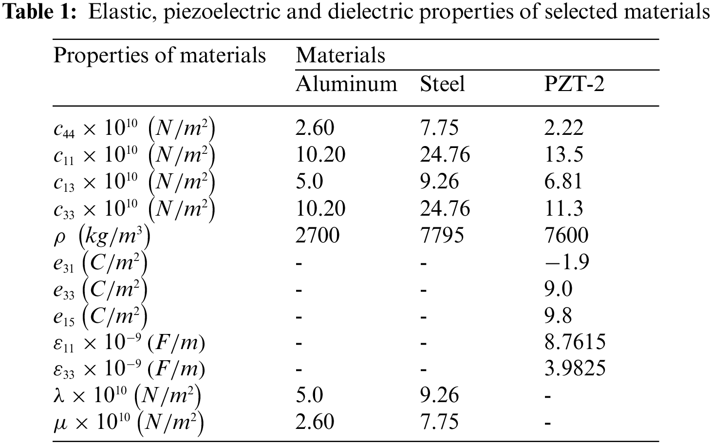
In the numerical investigations, steel and aluminum are selected as the metallic materials and PZT-2 as the piezoelectric material. According to Yang [44], the values of the physical-mechanical constants of these materials are given in Table 1. Glycerin is chosen as the fluid for which, according to Guz [8], the coefficient of viscosity, the density, and sound velocity are
We consider the numerical results related to the frequency response of the dimensionless normal stress
To begin, we consider the frequency response of the dimensionless interface stress
Let us now consider the graphs illustrated in Figs. 2–4 which show the frequency response of the stress and are constructed in the cases where
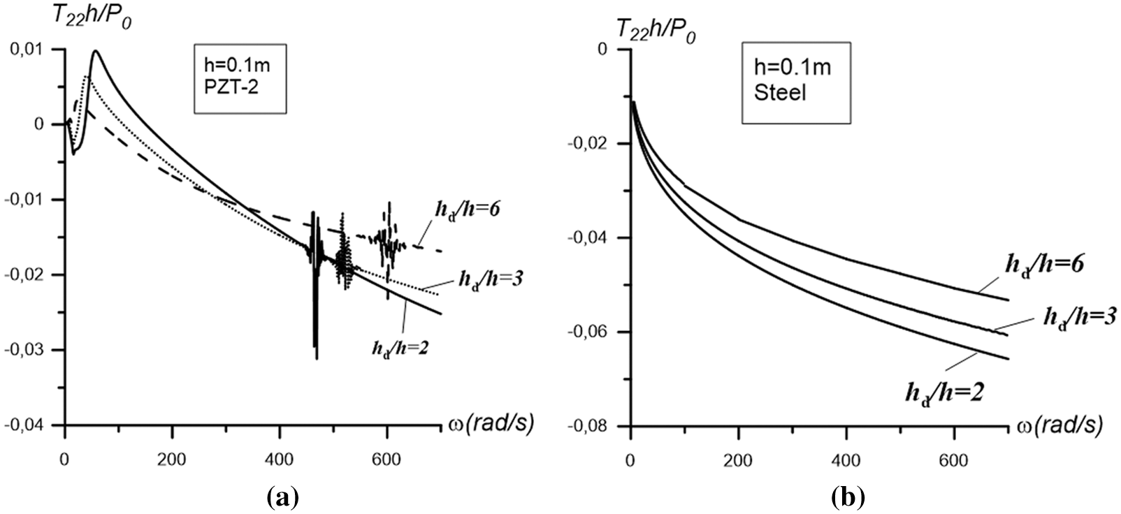
Figure 2: The graphs of the frequency response constructed for the interfacial stress at
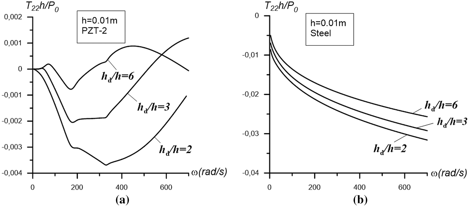
Figure 3: The graphs of the frequency response constructed for the interfacial stress at
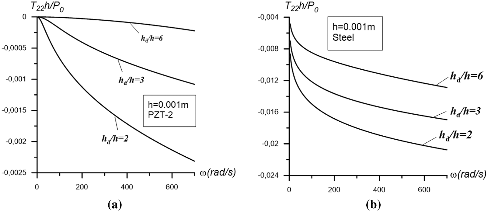
Figure 4: The graphs of the frequency response constructed for the interfacial stress at
From analysis of the results shown in Figs. 2b, 3b and 4b, i.e., from the results related to the case in which the plate is made only of metal, we can draw the following conclusions:
i. The graphs of the frequency response of the interfacial stress have a smooth character, and the absolute values of this stress increase monotonically with the vibration frequency.
ii. An increase in the thickness of the plate leads to an increase in the absolute values of the stress, and the character of the frequency responses constructed for different plate thicknesses is the same.
iii. An increase in the values of the ratio
From analysis of the results illustrated by the graphs in Figs. 2a, 3a, and 4a which refer to the case where the plate consists of only piezoelectric material, we can draw the following conclusions:
i. The character of the interface stress frequency response graphs depends significantly not only on the plate thickness, but also on the fluid depth, i.e., on the ratio
ii. For relatively large values of plate thickness, there is a low-frequency region of frequency change (denote this diapason as
iii. There is such a value of frequency
iv. Increasing the thickness of the plate generally leads to an increase in the absolute values of the stress.
v. For a relatively large plate thickness, a resonant frequency occurs for the considered hydro-elastic system and the values of the resonant frequencies increase with the ratio as well as with the plate thickness.
vi. The character of the influence of the ratio
vii. Comparison of the results for the metal plate case with the corresponding results for the piezoelectric plate shows that the absolute values for the metal plate are significantly higher than the corresponding values for the piezoelectric plate.
Consequently, piezoelectricity significantly complicates the frequency responses of the interfacial stress, not only in a quantitative sense, but also in a qualitative sense.
Now the question arises of how the mixture of metal and piezoelectricity affects the above frequency response. To answer this question, we consider and analyze the results presented in Figs. 5–7, obtained for the case
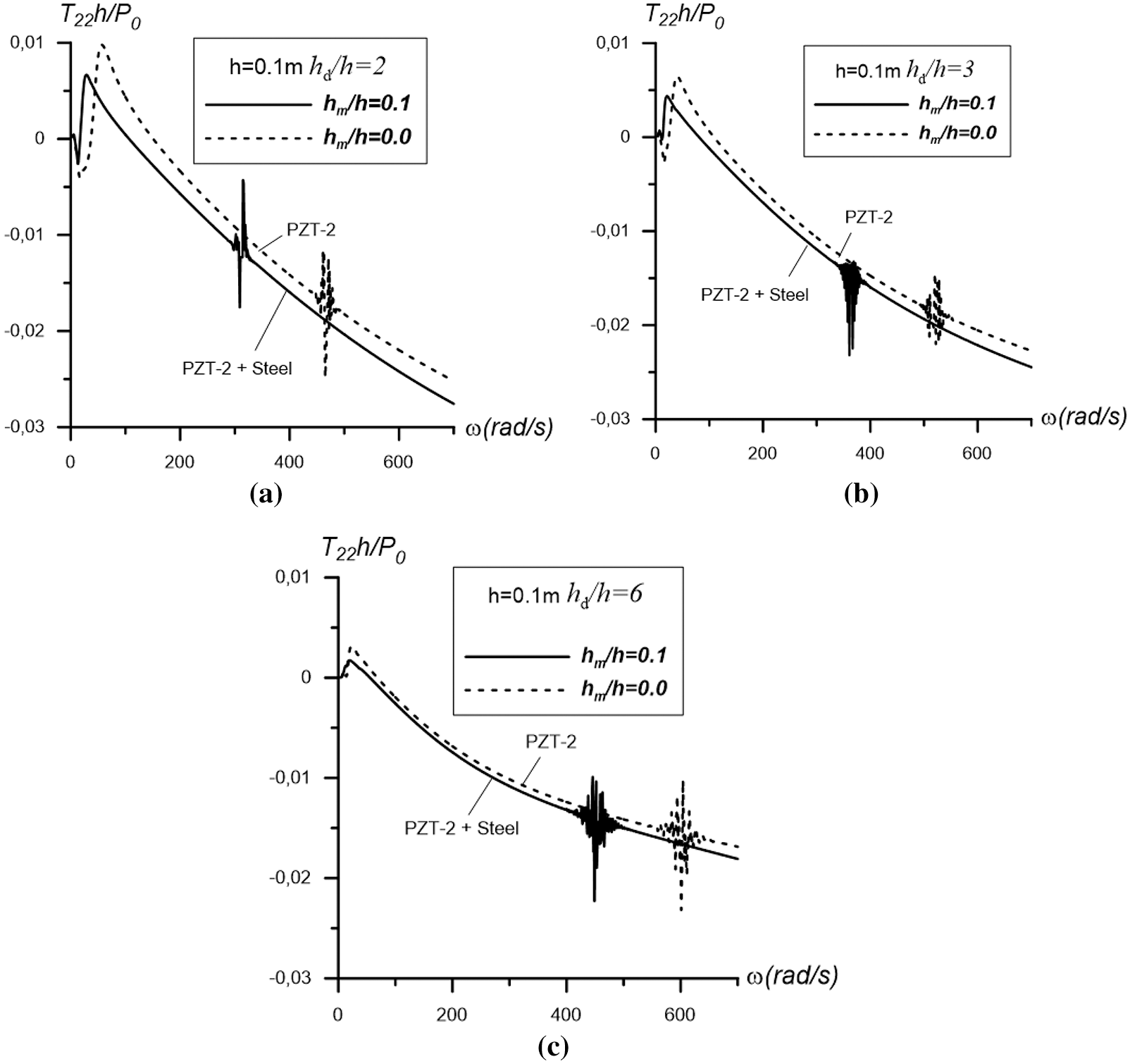
Figure 5: The graphs of the frequency response of the interfacial stress obtained under
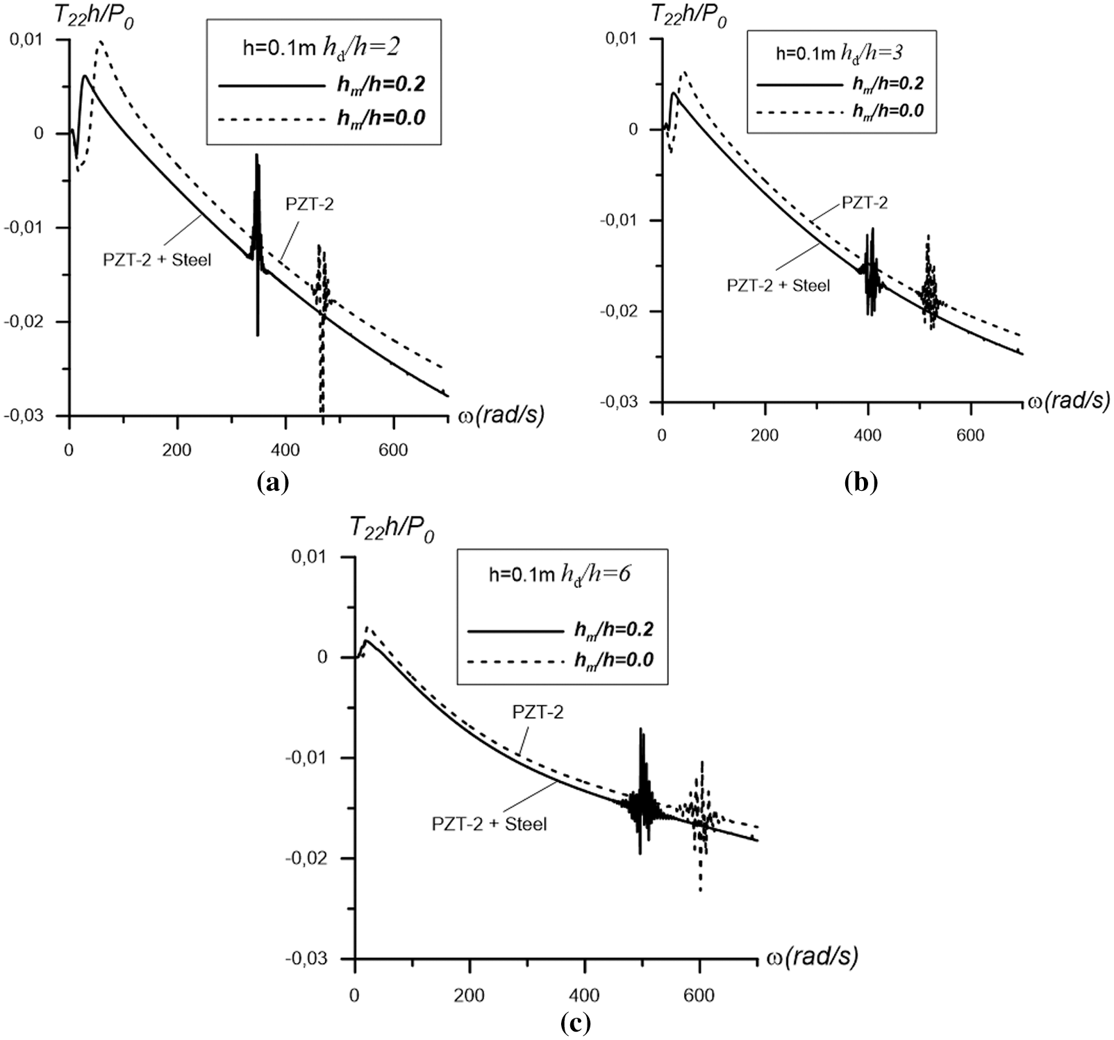
Figure 6: The graphs of the frequency response of the interfacial stress obtained under
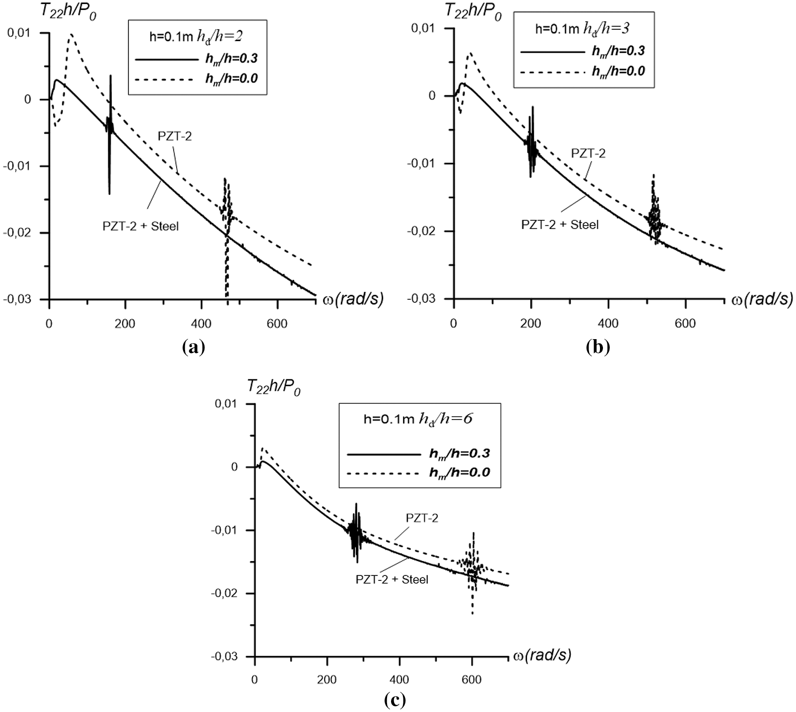
Figure 7: The graphs of the frequency response of the interfacial stress obtained under
We introduce the notation
At the same time, comparison of the results in Figs. 5–7 with each other show that an increase in the ratio
Recall that all the above results hold for the case where
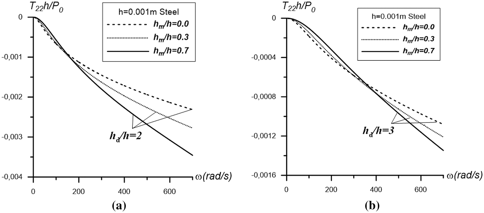
Figure 8: The influence of the ratio
These results are obtained for the cases with
Moreover, it is evident from these results that before (after) a certain value of this frequency, an increase in the values of the ratio
We have analyzed the results of the two-layer “steel+PZT-2” plate and all previous conclusions refer to this case. Now we consider some results shown in Fig. 9, which refer to the two-layer “aluminum+PZT-2” plate. Note that these results are obtained for the case where
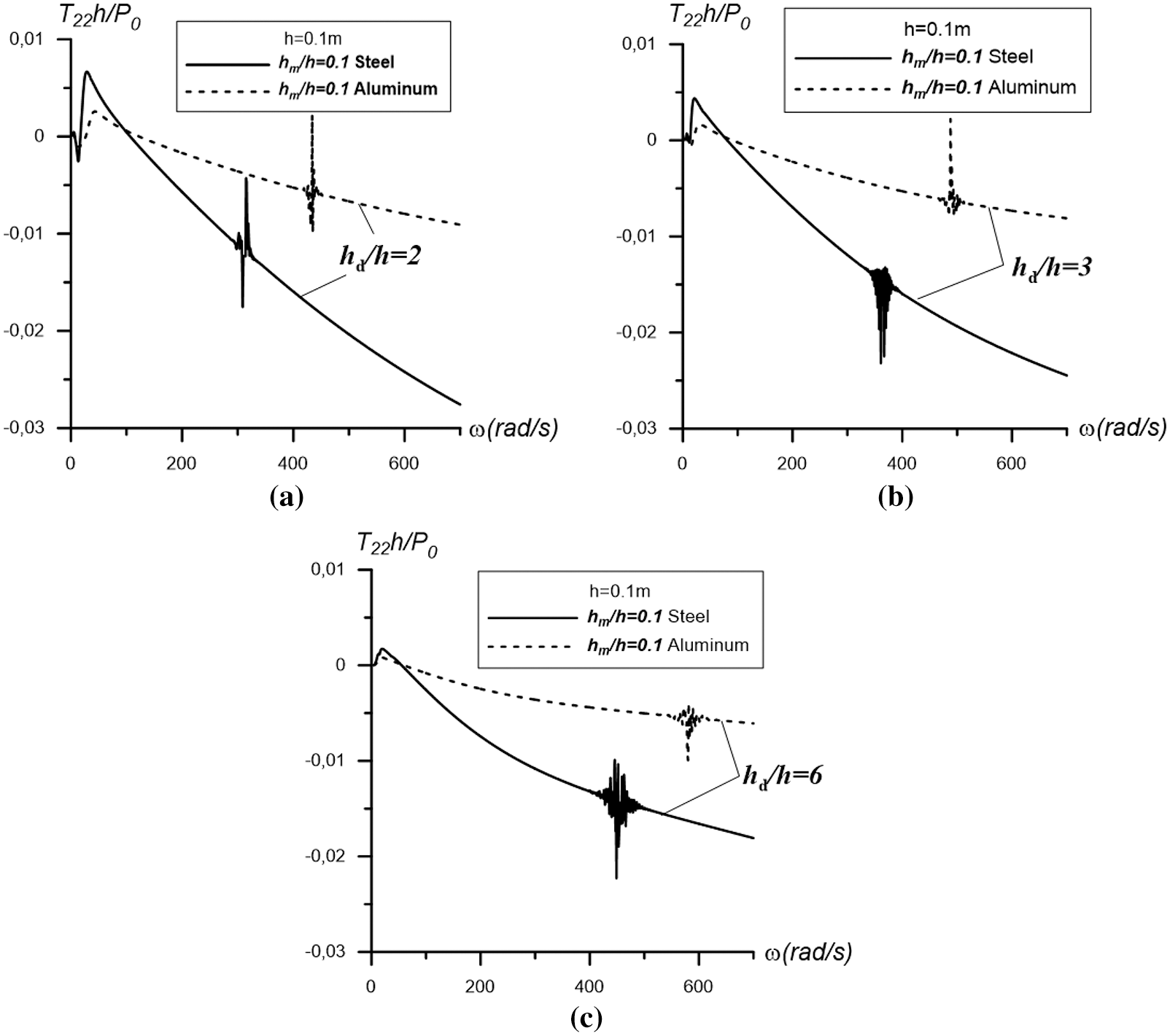
Figure 9: The graphs of the frequency response of the interfacial stress obtained under
Thus, it follows from the results in Fig. 9, that in the case of the “aluminum+PZT-2” plate, the D+RSR+BLD zone and the resonant frequency also appear. However, the “length” of this zone is less than, and the resonant frequency is greater than, in the case of the “steel+PZT-2” plate. At the same time, the absolute values of the interfacial stress obtained for the “aluminum+PZT-2” case are significantly lower than those of the “steel+PZT-2” plate. It can be concluded that the material properties of the metal layer can significantly influence the investigated frequency responses.
Finally, we consider the numerical convergence of the used computational algorithm within the framework of which the above results are obtained. Note that the convergence of the numerical results with respect to the length of the integration interval, i.e., with respect to
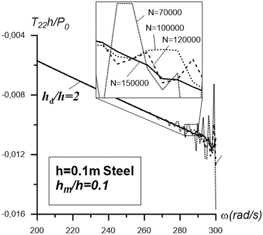
Figure 10: Examples of convergence of numerical results with respect to the number N obtained for the plate “Steel+PZT-2” in the case where
Thus, in the present work, the mechanically forced vibration of the hydro-elastic-piezoelectric system consisting of a two-layer “elastic+PZT” plate, a compressible viscous fluid, and a rigid wall has been investigated. The structure of this work is organized as follows: in Section 1, an overview and the findings of related research are given. In Section 2, the mathematical formulation of the problem, the equation of motion of the metal/PZT plate and the flow equations, as well as the corresponding boundary, contact, and compatibility conditions are given. In Section 3, the solution method for the formulated boundary value problem and the algorithm for obtaining numerical results are explained. The numerical results are presented and discussed in Section 4 and, finally, the results are summarized in the present section, i.e., in Section 5.
The PZT layer of the plate is assumed to be in contact with the fluid and time-harmonic linear forces act on the free surface of the elastic-metallic layer. The motion of the plate is described within the piecewise homogeneous body model using the exact equations and relations of elastodynamics and elasto-electrodynamics for piezoelectric materials. The fluid flow is described by the linearized Navier-Stokes equations for the barotropic, compressible, viscous Newtonian fluid. The plane-strain state in the plate and the plane flow in the fluid take place. For the solution of the corresponding boundary-value problem, the Fourier transform is used with respect to the spatial coordinate on the axis along the laying direction of the plate. The analytical expressions of the Fourier transform of all the sought values of each component of the system are determined. The origins of the searched values are determined numerically, after which the numerical results on the stress on the fluid and plate interface planes are presented and discussed.
These results are obtained for the case where PZT-2 is chosen as the piezoelectric material, steel and aluminum as the elastic metal materials, and glycerin as the fluid.
Analysis of these results allows the following concrete conclusions to be drawn about the character of the influence of the problem parameters on the frequency response of the stress acting on the interface between the piezoelectric layer and fluid:
− The character of the interface stress frequency response graphs obtained for the two-layer “metal+piezoelectric” plate depends significantly not only on the total thickness h of the plate, but also on the ratios
− At low vibration frequencies of the two-layer “metal+piezoelectric” plate and the plate consisting only of piezoelectric material (i.e., the “piezoelectric” plate), the zone “descent+relatively sharp rise+beginning of the last descent” (D + RSR + BLD) appears.
− Assuming that the D + RSR + BLD zone for the two-layer “metal+piezoelectric” plate appears for the frequencies
− As in the case where the plate is made of piezoelectric material only, and as in the case of the two-layer “metal+piezoelectric” plate, the resonance case occurs and the resonance frequency obtained for the two-layer “metal+piezoelectric” plate is lower than that obtained for the “piezoelectric” plate.
− The resonance frequency of the two-layer “metal+piezoelectric” plate decreases with the thickness of the metal layer in the plate.
− It is found that
− The differences
− The mechanical properties of the metal layer in the plate have a significant influence on the frequency response of the stress under investigation.
− Unfortunately, we did not find any related results from other authors with which to compare the present results. Therefore, we compared the obtained results with those of the authors of the present work for the cases where the materials of the plate layers are the same, i.e., the same metal material or the same PZT material.
− The above comparison shows that the concrete numerical results obtained are in agreement with known physical-mechanical considerations, and made it possible to control the magnitude of the interfacial pressure between the fluid and the plate by the choice of materials and the thickness of the plate layers.
In future works, an electrical field instead of mechanical force can be applied to the piezoelectric plate, so the mechanical response of the system can be analyzed. Furthermore, interface stress can be studied for different PZT and metal combinations.
Funding Statement: The authors received no specific funding for this study.
Conflicts of Interest: The authors declare that they have no conflicts of interest to report regarding the present study.
References
1. H. Lamb, “Axisymmetric vibration of circular plates in contact with water,” Proc. R Soc. (London) A, vol. 98, pp. 205–216, 1921. [Google Scholar]
2. M. Amabili, “Effect of finite fluid depth on the hydroelastic vibrations of circular and annular plates,” Journal of Sound and Vibration, vol. 193, pp. 909–925, 1996. [Google Scholar]
3. S. D. Akbarov, “Forced vibration of the hydro-vıscoelastic and–elastic systems consisting of the viscoelastic or elastic plate, compressible viscous fluid, and rigid wall: A review,”Applied and Computational Mathematics, vol. 17, no. 3, pp. 221–245, 2018. [Google Scholar]
4. S. D. Akbarov, Dynamics of Pre-Strained Bi-Material Elastic Systems: Linearized Three-Dimensional Approach, 1st ed., Cham Switzerland: Springer, pp. 1–997, 2015. [Google Scholar]
5. S. D. Akbarov and M. I. Ismailov, “Forced vibration of a system consisting of a pre-strained highly elastic plate under compressible viscous fluid loading,” CMES: Computer Modeling in Engineering & Sciences, vol. 97, no. 4, pp. 359–390, 2014. [Google Scholar]
6. S. D. Akbarov and M. I. Ismailov, “The forced vibration of the system consisting of an elastic plate, compressible viscous fluid, and rigid wall,” Journal Vibration and Control, vol. 23, no. 11, pp. 1809–1827, 2017. [Google Scholar]
7. S. D. Akbarov and M. I. Ismailov, “The influence of the rheological parameters of a hydro-viscoelastic system consisting of a viscoelastic plate, viscous fluid, and rigid wall on the frequency response of this system,” Journal Vibration and Control, vol. 24, no. 7, pp. 1341–1363, 2018. [Google Scholar]
8. A. N. Guz, Dynamics of Compressible Viscous Fluid. Cambridge, UK: Cambridge Scientific Publishers, 2009. [Google Scholar]
9. A. N. Guz, A. P. Zhuk and A. M. Bagno, “Dynamics of elastic bodies, solid particles, and fluid parcels in a compressible viscous fluid (Review),” International Applied Mechanics, vol. 52, no. 5, pp. 449–507, 2016. [Google Scholar]
10. V. N. Paimushin and R. K. Gazizullin, “Free and forced vibrations of a composite plate in a perfect compressible fluid, taking into account energy dissipation in the plate and fluid,” Lobachevskii Journal of Mathematics, vol. 42, no. 8, pp. 2016–2022, 2021. [Google Scholar]
11. V. N. Paimushin, D. V. Tarlakovskii, V. A. Firsov and R. K. Gazizullin, “Free and forced bending vibrations of a thin plate in a perfect compressible fluid with energy dissipation taken into account,” Z. Angew. Math Mech., vol. 100, no. 3, pp. e201900102, 2020. [Google Scholar]
12. M. Shuaib, M. Bilal, M. A. Khan and S. J. Malebary, “Fractional analysis of viscous fluid flow with heat and mass transfer over a flexible rotating disk,” CMES-Computer Modeling in Engineering & Sciences, vol. 123, no. 1, pp. 377–400, 2020. [Google Scholar]
13. S. V. Sorokin and A. V. Chubinskij, “On the role of fluid viscosity in wave propagation in elastic plates under heavy fluid loading,” Journal Sound and Vibration, vol. 311, pp. 1020–1038, 2008. [Google Scholar]
14. A. D. Zamanov, M. I. Ismailov and S. D. Akbarov, “The effect of viscosity of fluid on the frequency response of a viscoelastic plate loaded by this fluid,” Mechanics of Composite Materials, vol. 54, no. 1, pp. 41–52, 2018. [Google Scholar]
15. Y. Amini, H. Emdad and M. Farid, “Fluid-structure interaction analysis of a piezoelectric flexible plate in a cavity filled with fluid,” Scientia Iranica B, vol. 23, no. 2, pp. 559–565, 2016. [Google Scholar]
16. Y. Belkourchia, H. Bakhti and L. Azrar, “Numerical simulation of FSI model for energy harvesting from ocean waves and beams with piezoelectric material,” in Proc. of 6th Int. Renewable and Sustainable Energy Conf. (IRSEC), Rabat, Morocco, pp. 1–5, 2018. [Google Scholar]
17. F. Trentadue, G. Quaranta and C. Maruccio, “Energy harvesting from piezoelectric strips attached to systems under random vibrations,” Smart Structures and Systems, vol. 24, no. 3, pp. 333–343, 2019. [Google Scholar]
18. H. A. Zakaria and C. M. Loon, “The application of piezoelectric sensor as energy harvester from small-scale hydropower,” in Proc. of Int. Conf. on Civil and Environmental Engineering (ICCEE, 2018), Kuala Lumpur, Malaysia, pp. 521–528, 2018. [Google Scholar]
19. Y. H. Huang and H. T. Hsu, “Solid-liquid coupled vibration characteristics of piezoelectric hydroacoustic devices,” Sensors and Actuators A: Physical, vol. 238, pp. 177–195, 2016. [Google Scholar]
20. I. E. Kuznetsova, B. D. Zaitsev and I. A. Borodina, “Study of the hydroacoustic emitter based on the antisymmetric lamb wave in a piezoelectric ceramic plate,” Journal of Communications Technology and Electronics, vol. 56, no. 11, pp. 1382–1386, 2011. [Google Scholar]
21. V. Sharapov, S. Zhanna and L. Kunickaya, Piezo-electric Electro-Acoustic Transducers. Cham, Switzerland: Springer, pp. 57–71, 2014. [Google Scholar]
22. H. D. Akaydin, N. Elvin and Y. Andreoupoulos, “Harvesting from highly unsteady fluid flows using piezoelectric materials,” Journal of Intelligent Material Systems and Structures, vol. 21, pp. 1263–1278, 2010. [Google Scholar]
23. N. Elvin and A. Erturk, Advances in Energy Harvesting Methods, 1st ed., NY: Springer New York, 2013. [Google Scholar]
24. M. He, X. Zhang, L. S. Fernandes, A. Molter, X. Liang et al., “Multi-material topology optimization of piezoelectric composite structures for energy harvesting,” Composite Structures, vol. 265, pp. 113783, 2021. [Google Scholar]
25. Y. Chen and Z. Yan, “Nonlinear analysis of unimorph and bimorph piezoelectric energy harvesters with flexoelectricity,” Composite Structures, vol. 259, pp. 113454, 2021. [Google Scholar]
26. J. Jiang, S. Liu and L. Feng, “Improving functionality of 2 DOF piezoelectric cantilever for broadband vibration energy harvesting using magnets,” Energy Engineering, vol. 118, no. 5, pp. 1287–1303, 2021. [Google Scholar]
27. G. Nie and M. Wang, “Rayleigh-type wave in a rotated piezoelectric crystal imperfectly bonded on a dielectric substrate,” Computers, Materials & Continua, vol. 59, no. 1, pp. 257–274, 2019. [Google Scholar]
28. Y. Qiao, C. Zhang and J. Han, “Dynamic modeling and analysis of wind turbine blade of piezoelectric plate shell,” Sound & Vibration, vol. 53, no. 1, pp. 14–24, 2019. [Google Scholar]
29. Z. Ekicioglu Kuzeci, “Forced vibration of the system consisting of PZT layer, viscous fluid and rigid wall,” Ph.D. dissertation, Yildiz Technical University, Turkey, 2020. [Google Scholar]
30. A. M. S. Mahdy, M. Higazy and M. S. Mohammed, “Optimal and memristor-based control of a nonlinear fractional tumor-immune model,” CMC-Computer, Materials & Continua, vol. 67, no. 3, pp. 3463–3486, 2021. [Google Scholar]
31. K. A. Gepreel, A. M. S. Mahdy, M. S. Mohammed and A. Al-Amiri, “Reduced differential transform method for solving nonlinear biomathematics models,” CMC-Computer, Materials & Continua, vol. 61, no. 3, pp. 979–994, 2019. [Google Scholar]
32. O. Bazighifan, T. Abdeljawad and Q. M. Al-Mdallal, “Differential equations of even-order with p-laplacian like operators: Qualitative properties of the solutions,” Advances in Difference Equations, vol. 2021, no. 96, 2021. https://doi.org/10.1186/s13662-021-03254-7. [Google Scholar]
33. S. S. Santra, T. Ghosh and O. Bazighifan, “Explicit criteria for the oscillation of second-order differential equations with several sub-linear neutral coefficients,” Advances in Difference Equations, vol. 2020, no. 643, 2020. https://doi.org/10.1186/s13662-020-03101-1. [Google Scholar]
34. O. Bazighifan, T. H. Alotaibi and A. A. A. Mousa, “Neutral delay differential equations: Oscillation conditions for the solutions,” Symmetry, vol. 13, no. 1, pp. 101, 2021. [Google Scholar]
35. O. Bazighifan and P. Kumam, “Oscillation theorems for advanced differential equations with p-laplacian like operators,” Mathemetics, vol. 8, no. 5, pp. 821, 2020. [Google Scholar]
36. O. Moaaz, R. A. El-Nabulsi and O. Bazighifan, “Oscillatory behavior of fourth-order differential equations with neutral delay,” Symmetry, vol. 12, no. 3, pp. 371, 2020. [Google Scholar]
37. O. Bazighifan, “An approach for studying asymptotic properties of solutions of neutral differential equations,” Symmetry, vol. 12, no. 4, pp. 555, 2020. [Google Scholar]
38. O. Moaaz, E. M. Elabbasy and E. Shaaban, “Oscillation criteria for a class of third order damped differential equations,” Arab J. Math. Sci., vol. 24, no. 1, pp. 16–30, 2018. [Google Scholar]
39. O. Moaaz, D. Chalishajar and O. Bazighifan, “Some qualitative behavior of solutions of general class of difference equations,” Mathematics, vol. 7, no. 7, pp. 585, 2019. [Google Scholar]
40. A. M. S. Mahdy, K. Lotfy, A. El-Bary and H. H. Sarhan, “Effect of rotation and magnetic field on a numerical-refined heat conduction in a semiconductor medium during photo-excitation processes,” European Physical Journal Plus, vol. 136, no. 5, pp. 1–17, 2021. [Google Scholar]
41. M. S. Mohammed, K. Lotfy, A. El-Bary and A. M. S. Mahdy, “Photo-thermal-elastic waves of excitation microstretch semiconductor medium under the impact of rotation and initial stress,” Optical and Quantum Electronics, vol. 54, pp. 241, 2022. [Google Scholar]
42. A. K. Khamis, K. Lotfy, A. El-Bary, A. M. S. Mahdy and M. H. Ahmed, “Thermal-piezoelectric problem of a semiconductor medium during photo-thermal excitation,” Waves in Random and Complex Media, vol. 31, no. 6, pp. 2499–2513, 2020. [Google Scholar]
43. A. M. S. Mahdy, K. Lotfy and A. El-Bary, “Thermo-optical-mechanical excited waves of functionally graded semiconductor material with hyperbolic two-temperature,” European Physical Journal Plus, vol. 137, pp. 105, 2022. [Google Scholar]
44. J. Yang, An Introduction to the Theory of Piezoelectricity, 1st ed., NY: Springer New York, 2005. [Google Scholar]
45. F. Aylikci, S. D. Akbarov and N. Yahnioglu, “3D FEM analysis of buckling delamination of a piezoelectric sandwich rectangular plate with interface edge cracks,” Mechanics of Composite Materials, vol. 55, no. 6, pp. 797–810, 2020. [Google Scholar]
46. M. C. Ray, L. Dong and S. N. Atluri, “Simple efficient smart finite elements for the analysis of smart composite beams,” CMES-Computer Modeling in Engineering & Sciences, vol. 111, no. 5, pp. 437–471, 2016. [Google Scholar]
Cite This Article
 Copyright © 2023 The Author(s). Published by Tech Science Press.
This work is licensed under a Creative Commons Attribution 4.0 International License , which permits unrestricted use, distribution, and reproduction in any medium, provided the original work is properly cited.
 Downloads
 Citation Tools