Photovoltaic Models Parameters Estimation Based on Weighted Mean of Vectors

1  Introduction

Enhancing human life requires energy development and advancement. Therefore, the world’s focus has switched to renewable energy sources, including wind and solar, with the recent rise in fossil fuel prices [1]. Solar power is a feasible and promising alternative, and it has risen to prominence as one of the main significant forms of renewable energy in recent decades due to its availability, sustainability, and inexhaustibility [2]. Despite its numerous benefits, solar energy still needs further research and development to increase its efficiency [3]. So, researchers’ interest in enhancing renewable energy systems’ efficiency has grown in response to the rising interest in these sources. The development of an optimum mathematical model that represents the natural photovoltaic system is one of the most significant challenges for researchers [4]. This is due to the nonlinear properties of solar cells, so developing these models is a challenge [5]. As a result, accurate modeling of PV modules is essential to reflect their characteristics for further research [6]. According to scientific research in the field of PV system modeling, there are several types of PV models that may be used to represent the PV cell or module [7]. One of these models is the static model, which is considered the basic element of a photovoltaic system since it relies on the principal features of a photovoltaic cell, which comprises two semiconductor materials (p-type and n-type) to attain simple PN junction properties [8].

The single diode model (SDM) is the simplest static model, which consists of one diode connected by series and shunt resistance [9]. By adding an extra diode to the previous model, the double diode module (DDM) is created, which consists of two diodes connected by a resistor in shunt and another in series [10]. As a result, it is more intricate than SDM, as the total parameters estimated in DDM are seven, whereas in SDM they are five [11]. Further effects can be modeled by increasing the number of diodes, which increases model accuracy [12]. However, the estimated parameters for the model are also increased, leading to increased model complexity [13]. The three-diode model (TDM) illustrates this concept. The impact of leakage current and grain boundaries is represented by three diodes in TDM [14]. Because TDM includes nine estimated parameters, it is regarded as more complicated, even if it is more accurate. According to the application, the balance between correctness and complexity is defined [15]. Despite the static model having seen a variety of advancements in the previous studies and is more representative of the PV system, the load connection, variability, and switch are not represented. To overcome this problem, the dynamic model, which reflects the load connection in the model, has been presented in the literature. In the literature, the integer and fractional dynamic models have been suggested. The most prevalent dynamic model is the integer model, while the fractional model was established to enhance the integer model’s accuracy [16]. The parameters for each model are different. These parameters have an impact on the model’s output. The accuracy of the model is directly affected by the correctness of these parameters, which many scholars have offered to debate. Several researchers have used optimization approaches to study parameter estimation. An overview of the optimization techniques used to estimate PV model parameters is proposed in [17]. For optimization issues, numerical/analytical approaches are used, although these methods produce low-precision solutions. For these situations, population-based algorithms are extensively used because they are easier to implement and produce more accurate answers. There are far too many population-based algorithms to cover in this work, but one example includes the Moth-Flame Optimization (MFO) algorithm [16], Water Cycle Algorithm (WCA) [18], Enhanced Vibration of Particles System (EVPS) [19], Harris Hawks Optimization (HHO) [20], Shued Frog Leaping (SFL) algorithm [21]. Logically, the No Free Lunch (NFL) theorem [22] establishes that there is no metaheuristic optimization strategy that can solve all optimization issues. Per this theorem, an optimizer’s superior performance in a single category of issues does not ensure similar performance in another. This theorem is at the heart of a lot of studies in the literature, and it allows researchers to adapt existing approaches to new sorts of problems. The goal of this research is to provide an effective search technique for estimating the un-known parameters of PV cells and discussing them through a recent optimizer (INFO). The presented different models of PV systems such as static models (SDM, and DDM) and different dynamic models (IOM, and FOM) that are not discussed in other references such as [23]. The INFO algorithm has strong performance in parameter optimization, which has been proven in [24]. The INFO algorithm provides several advantages over other algorithms, including faster convergence speed, solution accuracy, and balance, as well as excellent performance in parameter optimization and achieving excellent results in engineering experiments, which has been proven in [24]. Therefore, all of the above served as the basis and motivation for this study to use INFO to overcome this issue. This is the basis and motivation for this study to use INFO to overcome this issue. This article’s major contributions are summarized as follows:

•   Estimating the parameters of various PV models, including static and dynamic PV models, using the INFO algorithm as well as other well-known optimization algorithms.

•   On the same data set for the RadioTechnique Compelec (R.T.C) France solar cells, parameters extracted from another optimization algorithm were compared with the proposed the INFO algorithm.

•   The comparative algorithms were evaluated for their best performance using the best RMSE values, as well as their convergence and durability curves, to identify which algorithm was the fastest and most efficient.

•   The proposed INFO algorithm’s performance was compared to other algorithms using statistical analysis.

•   The efficiency of the proposed INFO was validated by calculating the value of the absolute error of the current and power at the best root mean square.

The remainder of this work is arranged as follows: The static and dynamic PV models are presented in Section 2. The INFO algorithm is introduced in Section 3. Section 4 discusses the results and evaluation. The conclusion is presented in Section 5.

2  Photovoltaic Models Analysis

A rigorous determination of the electric properties of the PV device under general ambient circumstances is necessary for appropriate PV system design [25]. This is accomplished by developing a precise comparable model for this device. Many mathematical models are suggested in the literature to describe the functioning and behavior of PV models [16]. The far more prevalent static and dynamic models are discussed in this section.

2.1 Static Photovoltaic Models

The static PV models SDM and DDM are commonly used to illustrate PV module (I-V) attributes. Because of its simplicity, SDM is the most often used model [26]. It consists of one diode connected by series and shunt resistance (Rs, Rsh) to the photo-generated current (Iph), which is expressed by a current source parallel-connected with the diode. SDM is the simplest model since it just includes five parameters. Assume x is a model parameters vector x = (x1, x2, x3, x4, x5) identical to (Rs, Rsh, Iph, Is, ɳ). Fig. 1 depicts the SDM equivalent circuit, which is represented by Eqs. (1) and (2) [27]. Where I is the solar cell output current, Ish is the shunt current, ID is the diode saturation current, Isd denotes the reverse saturation current, V is the terminal output voltage, ɳ is the ideality factor, k is Boltzmann’s constant, q is the electronic charge, and T is the cell absolute temperature in K. The DDM is a more intricate model devised to describe the impact of recombination in the PV cell, and it is accomplished by adding an additional diode to the SDM circuit, as illustrated in Fig. 2. The DDM contains seven parameters: x = (x1, x2, x3, x4, x5, x6, x7), which are identical to (Rs, Rsh, Iph, Is1, Is2, ɳ1, ɳ2), and expressed by Eqs. (3) and (4), while the objective functions for both SDM and DDM are expressed by Eqs. (5) and (6), respectively [28].

I=Iph−ID−Ish(1)

I=Iph−Isd[exp⁡(q(V+IRs)ηKT)−1]−(V+IRs)Rsh(2)

I=Iph−ID1−ID2−Ish(3)

I=Iph−Isd1[exp⁡(q(V+IRs)η1KT)−1]−Isd2[exp⁡(q(V+IRs)η2×KT)−1]−(V+IRs)Rsh(4)

fSD(V,I,X)=I−X3+X4[exp⁡(q(V+IX1)X5KT)−1]+(V+IX1)X2(5)

fDD(V,I,X)=I−X3+X4[exp⁡(q(V+IX1)X6KT)−1]+X5[exp⁡(q(V+IX1)X7KT)−1]+(V+IX1)X2(6)

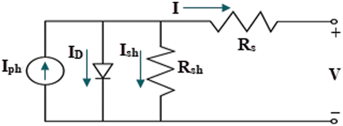
Figure 1: SDM equivalent model

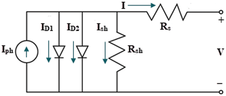
Figure 2: DDM equivalent model

2.2 Dynamic Photovoltaic Models

There are two notable dynamic PV models reported in the literature that will be discussed in this section: the integral and fractional dynamic photovoltaic models.

The integral order dynamic photovoltaic model (IOM) is a dynamic second-order model of the PV module and its connected load. The static part is minimized to a constant source voltage V and series resistance Rs, while the dynamic part is expressed by a capacitor C for the capacitance of the junction and the resistance Rc for the conduction, as displayed in Fig. 3. The inductance of connected cables is portrayed by the coil inductance L and the load is expressed by RL. IOM’s overall number of unknown parameters is three (Rc, C, and L). The IOM is expressed by Eqs. (7) and (8).

iL(s)=VOCsa21(s+b1)+b2(s−a11)(s−a22)(s−a11)−a12a21(7)

(a11a12a21a22)=(−1C(RC+RS)−RSC(RC+RS)RSL(RC+Rs)−[RLRC+RSRC+RLRS]L(RC+RS))(8)

(b1b2)=(1C(RC+RS)RCL(RC+RS))

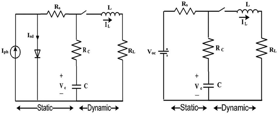
Figure 3: IOM equivalent model

The fractional-order dynamic photovoltaic model (FOM) was developed to describe fractional capacitors when Rc has a low value due to real frequency dependence on fractional capacitance impedance, as shown in Fig. 4. Capacitance and inductance are expressed in fractional order by α and β respectively. FOM’s overall number of unknown parameters is five (Rc, C, L, α, and β). The FOM is represented by Eqs. (9) and (10).

iL(s)=VOCsa21(sα+b1)+b2(sα−a11)(sβ−a22)(sα−a11)−a12a21(9)

(a11a12a21a22)=(−1Cα(RC+RS)−RSCα(RC+RS)RSLβ(RC+Rs)−[RLRC+RSRC+RLRS]Lβ(RC+RS))(10)

(b1b2)=(1Cα(RC+RS)RCLβ(RC+RS))

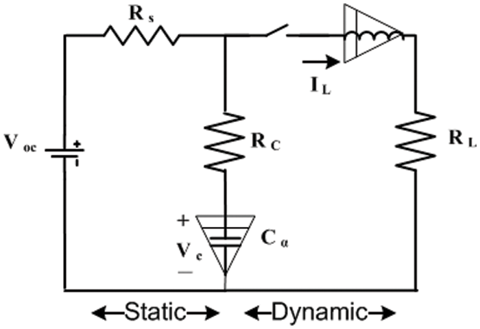
Figure 4: FOM equivalent model

3  Optimization Methodology

WeIghted meaN oF vectrOrs (INFO) is metaheuristic algorithm that search for the best solutions based on a calculation of the mean of weights for some vectors in the search area of the problem. The INFO has three main stages updating rules, vector merging and local search.

3.1 Updating Rules Stage

In this stage new rules have been updated. Firstly, INFO uses some random vectors. To move to the better solutions, based on the obtained solutions the mean rule between best, better and worst solutions, is determined as follow:

meanrule=r×WM1lg+(1−r)×WM2lg(11)

l=1,2,…,Np

WM1lg=δw1(xa1−xa2)+w2(xa1−xa3)+w3(xa2−xa3)w1+w2+w3+ε+ε×rand,(11.1)

l=1,2,…,Np

where

w1=cos⁡((f(xa1)−f(xa2))+π)×exp⁡(−f(xa1)−f(xa2)ω)(11.2)

w2=cos⁡((f(xa1)−f(xa3))+π)×exp⁡(−f(xa1)−f(xa3)ω)(11.3)

w3=cos⁡((f(xa2)−f(xa3))+π)×exp⁡(−f(xa2)−f(xa3)ω)(11.4)

ω=max(f(xa1),f(xa2),f(xa3))(11.5)

WM2lg=δw1(xbs−xbt)+w2(xbs−xws)+w3(xbt−xws)w1+w2+w3+ε+ε×rand,(11.6)

l=1,2,…,Np

where

w1=cos⁡((f(xbs)−f(xbt))+π)×exp⁡(−f(xbs)−f(xbt)ω)(11.7)

w2=cos⁡((f(xbs)−f(xws))+π)×exp⁡(−f(xbs)−f(xws)ω)(11.8)

w3=cos⁡((f(xbt)−f(xws))+π)×exp⁡(−f(xbt)−f(xws)ω)(11.9)

ω=f(xws)(11.10)

where f(x) is the objective function, a1,a2,a3 and l are unequal integer random values within range [1, Np]; ε is constant xbs,xbt and xws are best , better and worst solutions respectively for gth generation; r is random value within range [0, 0.5]; w1,w2 and w3 are three weights used to calculate the mean weight. The scaling factor of (δ) in the mean rule equation is calculated as follow:

δ=2β×rand−β(12)

where

β=2exp⁡(−4×gMaxg)(12.1)

where Maxg is the maximum number of generations. The acceleration part of convergence (CA) is described as follow:

CA=randn×(xbs−xa1)(f(xbs)−f(xa1)+ε)(13)

where randn is a constant for normal distribution random number. The new vector is calculated as follow:

Zlg=xlg+σ×mean rule+CA(14)

The updating rules through the exploration phase can be described as follow:

if rand < 0.5

Z1lg=xlg+σ×mean rule+randn×(xbs−xa1g)(f(xbs)−f(xa1g)+1)

Z2lg=xbs+σ×mean rule+randn×(xa1g−xa2g)(f(xa1g)−f(xa2g)+1)

else

Z1lg=xag+σ×mean rule+randn×(xa2g−xa3g)(f(xa2g)−f(xa3g)+1)

Z2lg=xbt+σ×mean rule+randn×(xa1g−xa2g)(f(xa1g)−f(xa2g)+1)

end(15)

where Z1lg and Z2lg are the new vectors and σ is the scaling factor which can be described as follow:

σ=2α×rand−α(16)

where

α=cexp⁡(−d×gMaxg)(16.1)

where c and d are constants

3.2 Vector Combining

In this stage a selection of new best rules has been implemented by combination between the last calculated rules (Z1lg and Z2lg). The combination between rules has been implemented based the following equations:

if rand<0.5

Ulg=Z1lg+μ.|Z1lg−Z2lg|(17)

else

Ulg=Z2lg+μ.|Z1lg−Z2lg|(17.1)

end

else

Ulg=xlg(17.2)

end

where the Ulg is the new obtained rules; μ=0.5×randn.

3.3 Local Search

In this stage a deep search has been implemented to search for the global best solution. The deep search has been implemented based on the following equations:

if rand<0.5

if rand<0.5

Ulg=xbs+randn×(mean rule+randn×(xbsg−xa1g))(18)

else

Ulg=xrnd+randn×(mean rule+randn×(υ1×xbs−υ2×xrnd))(18.1)

end

end

where

xrnd=ϕ×xavg+(1−ϕ)×(ϕ×xbt+(1−ϕ)×xbs)(18.2)

where

xavg=xa+xb+x33(18.3)

where ϕ is a random number within range [0, 1]. xrnd is the new solution; υ1and υ2 are two random numbers described as follow:

υ1={2×randif p>0.51otherwise}(18.4)

υ2={randif p>0.51otherwise}(18.5)

where p is a random number within range [0, 1]. The flowchart of the INFO algorithm is described in Fig. 5 [24]:

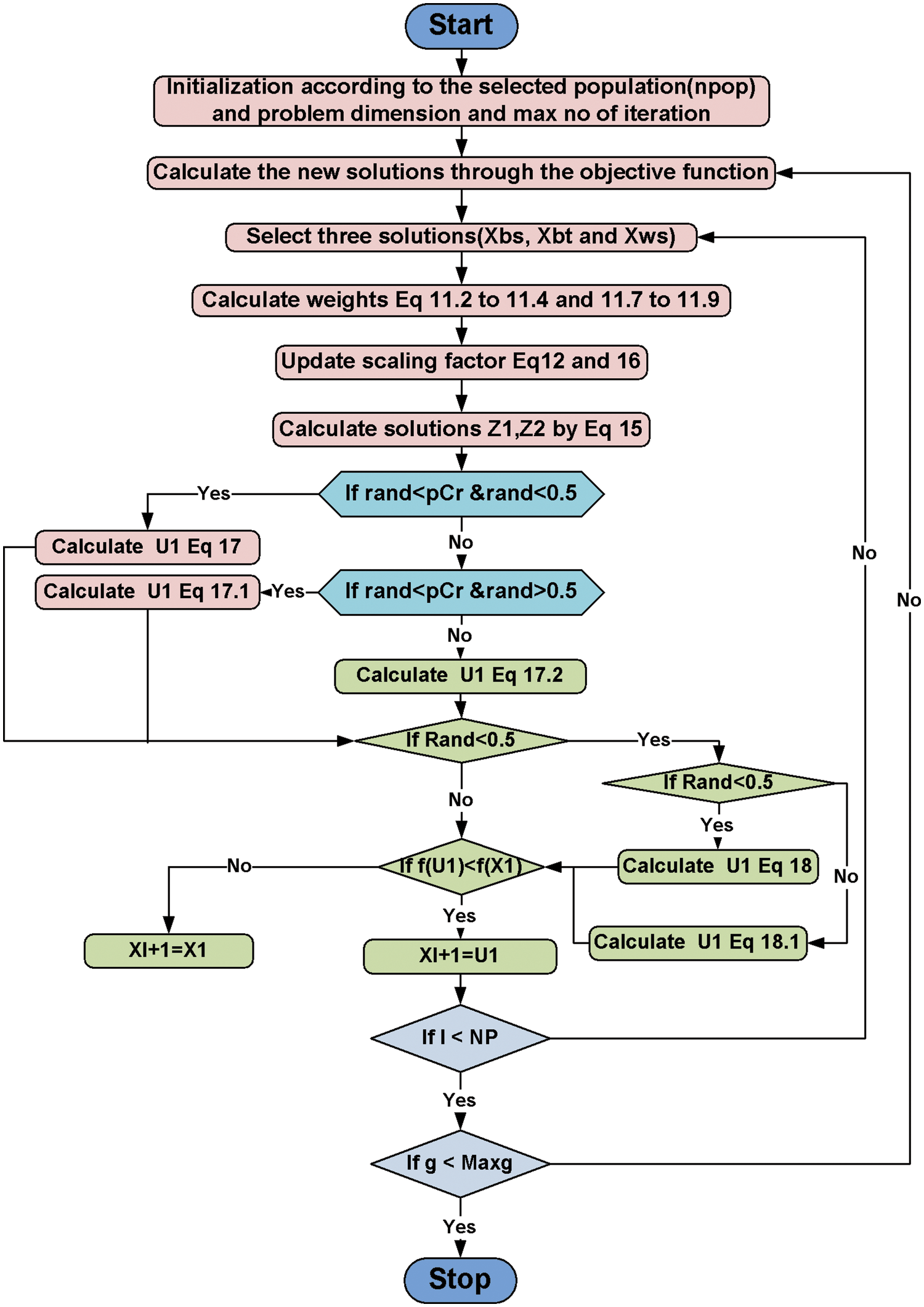
Figure 5: Weighted mean of vectors (INFO) flowchart

4  Results and Evaluation

Numerical simulations of the suggested INFO technique for identifying the parameters of both models (static and dynamic) of the PV module are illustrated in this section through different scenarios. The outcomes of parameters estimation operation for static SDM and DDM are introduced in Scenario 1. Scenario 2 shows the outcomes of the dynamic IOM and FOM parameters estimate operation.

4.1 Scenario_1

This scenario discusses the results and assessment of the procedures for determining the SDM and DDM parameters of the R.T.C France 57 mm diameter silicon merchant solar cell. The data were collected from the cell at a temperature of 33°C and at irradiation of 1000 W/m2 [29].

The INFO-based parameters estimate was performed on a MATLAB 2020a platform with an Intel® core TM i5-4210U CPU running at 1.70 GHz and 8 GB of RAM. The estimating operation was applied by INFO and compared with some contemporary algorithms. The compared algorithms were Gradient-Based Optimizer (GBO) [30], Runge Kutta Optimizer (RUN) [31], Harris hawks optimization (HHO) [32], Moth-Flame Optimization Algorithm (MFO) [17], and Black Widow Optimization Algorithm (BWOA) [33]. Table 1 illustrates the upper and lower limitations for all calculated parameters. Table 2 illustrates the control settings and number of population (np) for all the algorithms that were compared. To compute the best performance of the examined algorithms and the decision parameters for different PV models. The best RMSE values of the comparative algorithms have been obtained using the current’s measured actual data (Imeasured) corresponding to the voltage’s measured actual data (V), and the current’s estimated data (Iestimated,) based on the model parameter values estimated by all algorithms (X) in Eq. (19). The computed parameters of both SDM and DDM by INFO and other techniques are displayed in Tables 3 and 4, respectively. For SDM, the best RMSE was shared by the INFO, HHO, and GBO algorithms, followed by the RUN, MFO, and BWOA algorithms. For DDM, the INFO algorithm had the lowest RMSE, followed by the GBO method. To identify the fastest and most efficient algorithm, the convergence curve of all studied methods for SDM is displayed in Fig. 6. The convergence curve of all studied methods for DDM is displayed in Fig. 7. The INFO attained the best behavior of convergence for DDM, which can be seen in Fig. 7. To determine the robustness of the suggested method and compared methods, RMSE data were statistically evaluated to compute the fitness function’s maximum, minimum, standard deviation, and mean. The accuracy and robustness of any algorithm rely on the minimum and standard deviation values of root mean square error (RMSE), respectively. Tables 5 and 6 provide the statistical analysis of 50 independent runs of all examined algorithms for SDM and DDM, respectively, while Fig. 8 displays their graphical analysis using boxplot illustrations. The INFO has the lowest standard deviation (STDEV), indicating that it is the most stable and resilient. For a detailed evaluation of the generated models’ performance based on variables estimated by the examined algorithms. Figs. 9 and 10 demonstrate a comparison between the measured PV characteristic curves for current-voltage and power-voltage with those estimated by various models for SDM and DDM, respectively. Figs. 11 and 12 also provide further evaluation data for SDM and DDM, respectively, based on the calculation of current absolute error (Eq. (20)), and power absolute error (Eq. (21)) between the real measured values (Imeasured, and Pmeasured) and the estimated values (Iestimated, and Pestimated) for current and power, respectively. According to the outcomes in Figs. 11 and 12, both SDM and DDM respectively achieved an absolute error of (1.8039425002586E-05 and 5.8081141266486E-06) for power and (8.7697739438952E-05 and 2.823584893851E-05) for current. In the comparison of the preceding figures, the INFO outperformed other algorithms, whereas the outcomes for DDM were more accurate than SDM.

RMSE=1N∑i=1N(Imeasured(V)−Iestimated(V,X))2(19)

Current Absolute Error=∑1N(Imeasured−Iestimated)22(20)

Power Absolute Error=∑1N(Pmeasured−Pestimated)22(21)

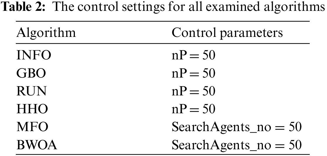
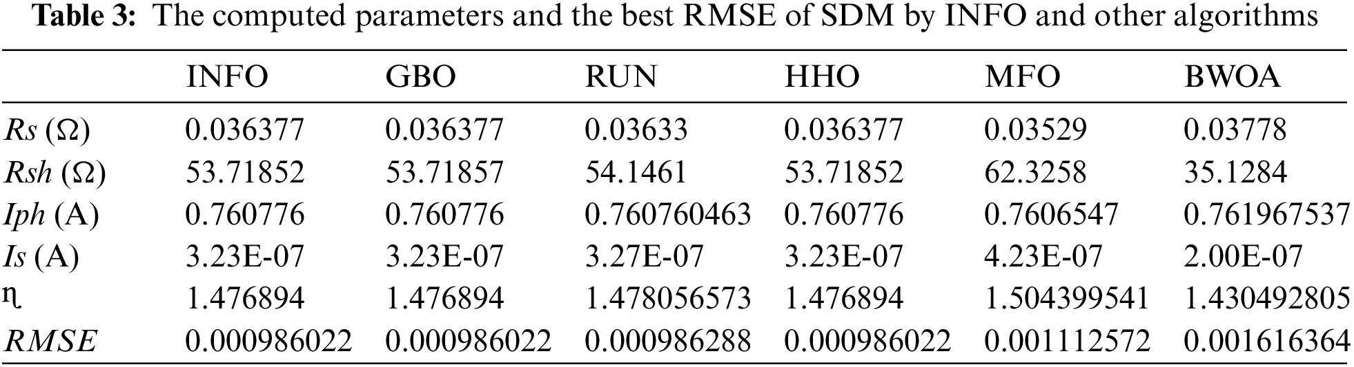
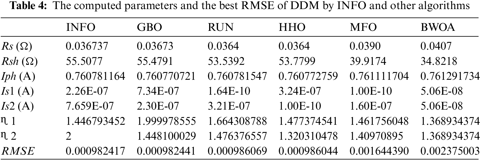
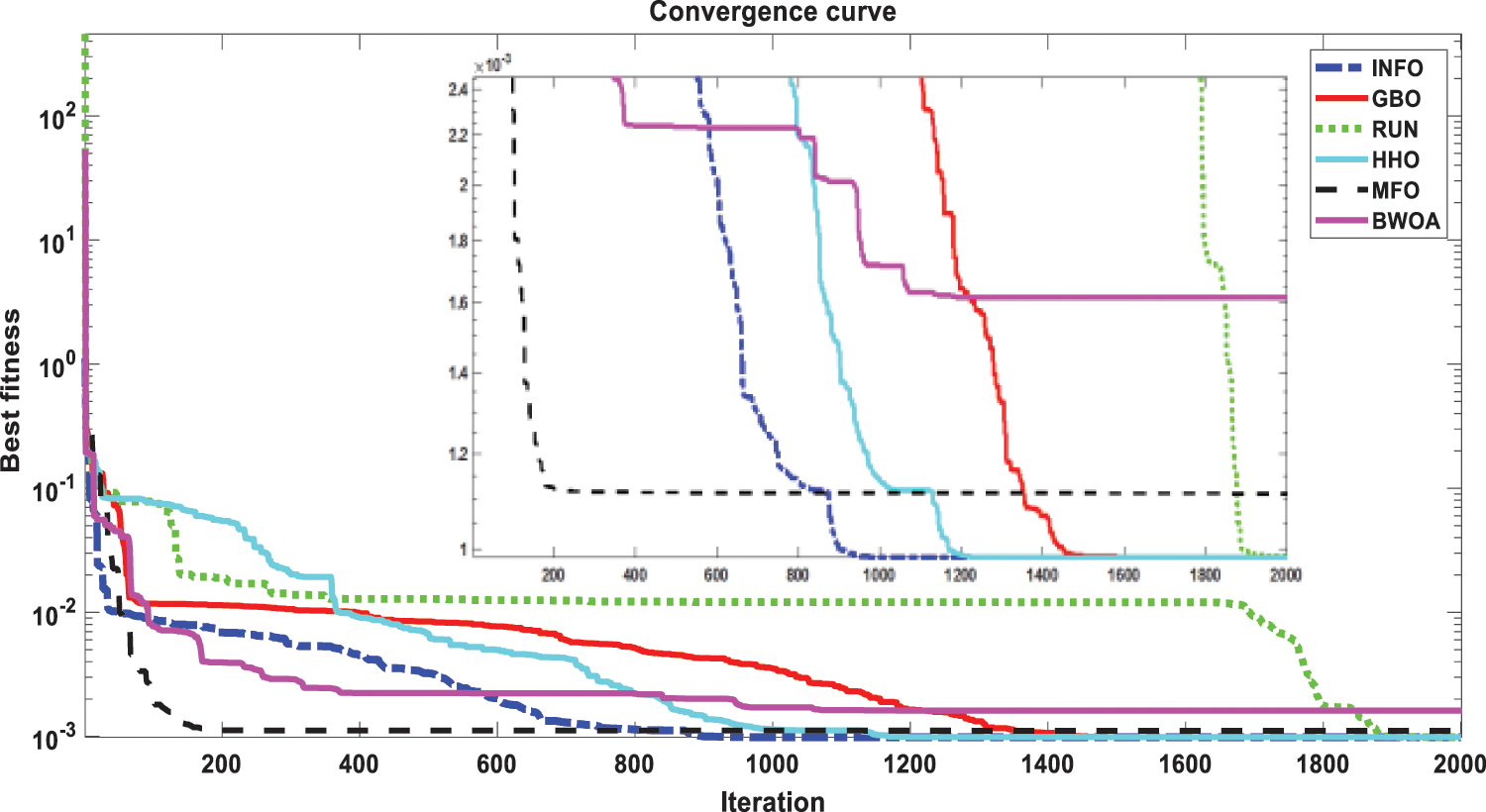
Figure 6: Convergence curves of various investigated algorithms for SDM

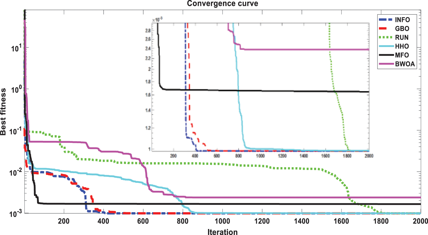
Figure 7: Convergence curves of various investigated algorithms for DDM

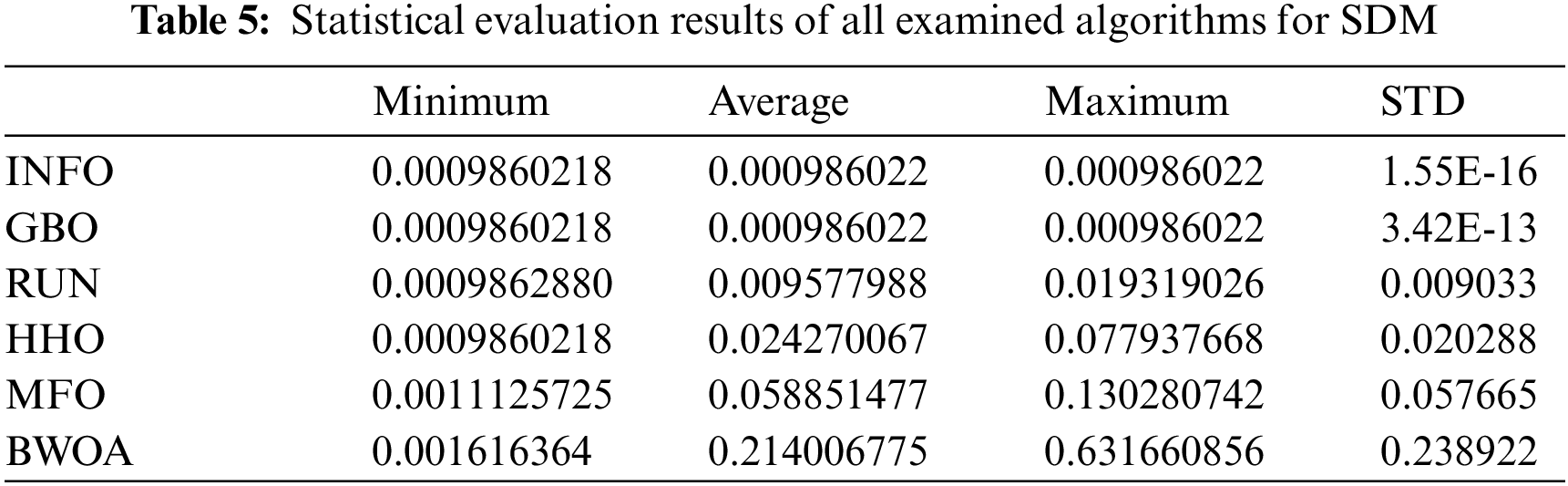
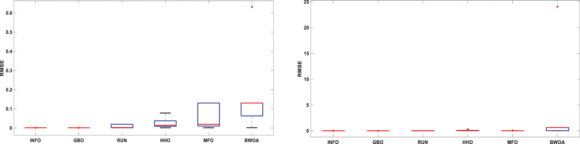
Figure 8: Boxplot illustrations of all the investigated algorithms, over both SDM and DDM, during 50 separate runs

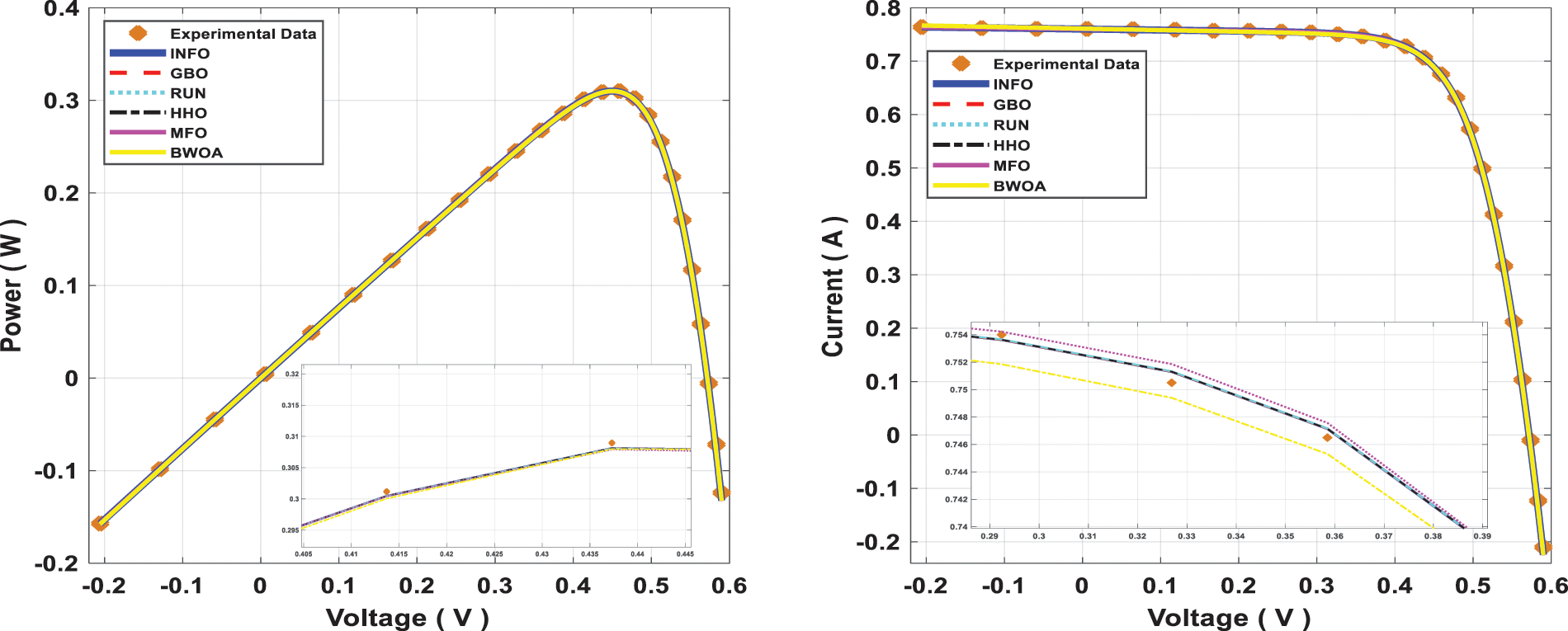
Figure 9: Power and current characteristics for computed SDM through all studied algorithms

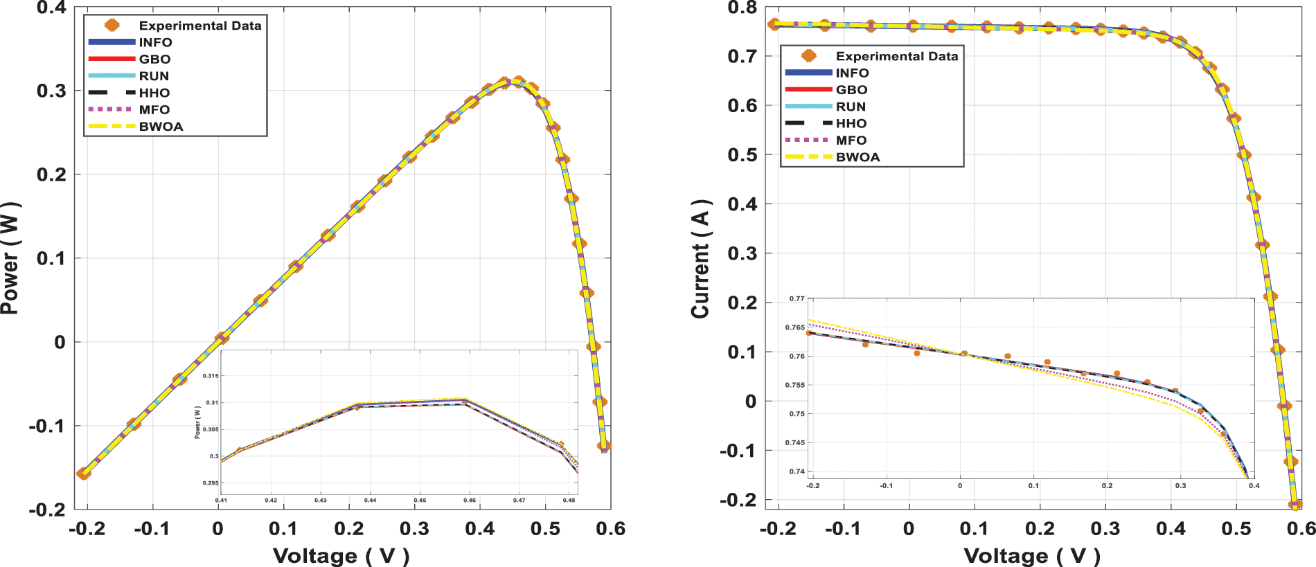
Figure 10: Power and current characteristics for computed DDM through all studied algorithms

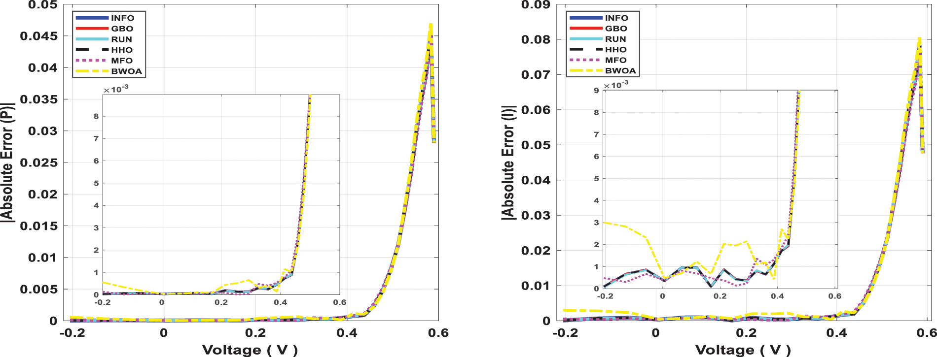
Figure 11: Power and current absolute error for computed SDM through all studied algorithms

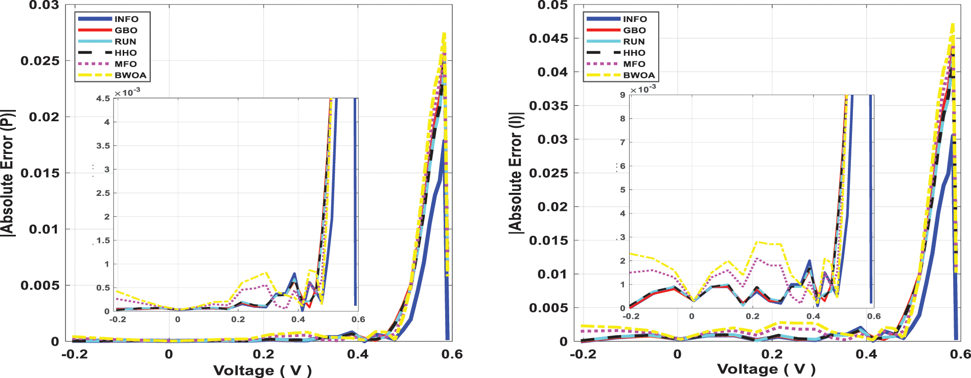
Figure 12: Power and current absolute error for computed DDM through all studied algorithms

4.2 Scenario_2

This scenario focuses on the use of INFO to estimate parameters in both dynamic PV models (IOM and FOM). Based on a dynamic experimental dataset of the load current for the connected PV module with load RL = 23.1 Ω at a temperature of 25°C with an irradiation level of 655 W/m2, the parameters of both IOM and FOM are extracted [34]. Table 7 illustrates the upper and lower ranges for all calculated parameters. In Table 8 the three computed parameters for IOM (Rc, C, and L) as well as the lowest RMSE obtained by all algorithms are presented. Table 9 displays the five estimated FOM parameters (Rc, C, L, α, and β) as well as the least RMSE achieved by all algorithms. The best RMSE was shared by all compared algorithms except for BWOA and HHO algorithms. For FOM, the INFO algorithm had the best RMSE, followed by the RUN and GBO algorithms, respectively. In Figs. 13 and 14, the convergence curves of various investigated techniques for IOM and FOM are displayed to define which algorithm was the most efficient and rapid. Figs. 15 and 16 exhibit a comparison between the load current for genuine experimental data with those estimated by all examined techniques for IOM and FOM, respectively. Figs. 17 and 18 also provide further evaluation data for IOM and FOM, respectively, based on the computation of the current absolute error between the real measured values and the estimated values through all techniques. According to the outcomes in Figs. 17 and 18, current achieves an absolute error of (1.49374083879827E-06 and 6.67252610941915E-07) for IOM and FOM, respectively. In the comparison of the preceding figures, the INFO’s performance was superior to other algorithms, while the outcomes for FOM were more precise than for IOM.

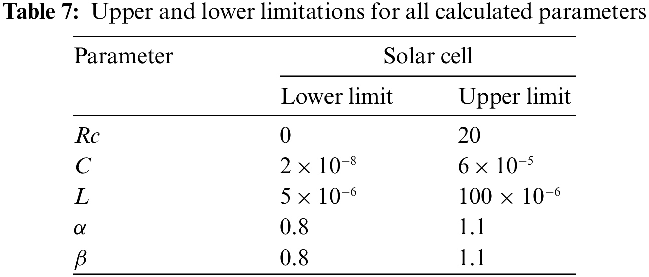
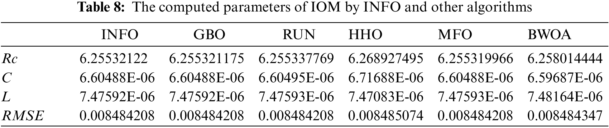
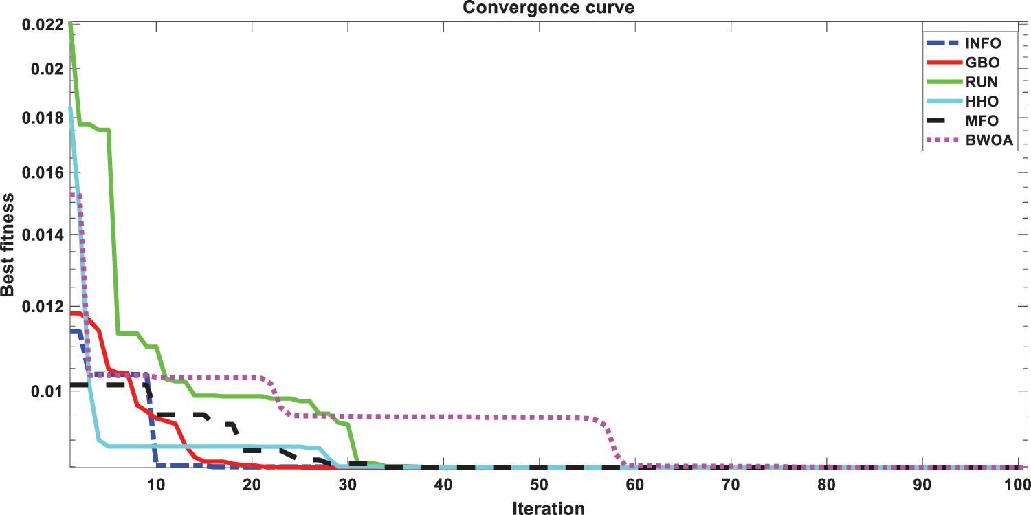
Figure 13: Convergence curves of various investigated algorithms for IOM

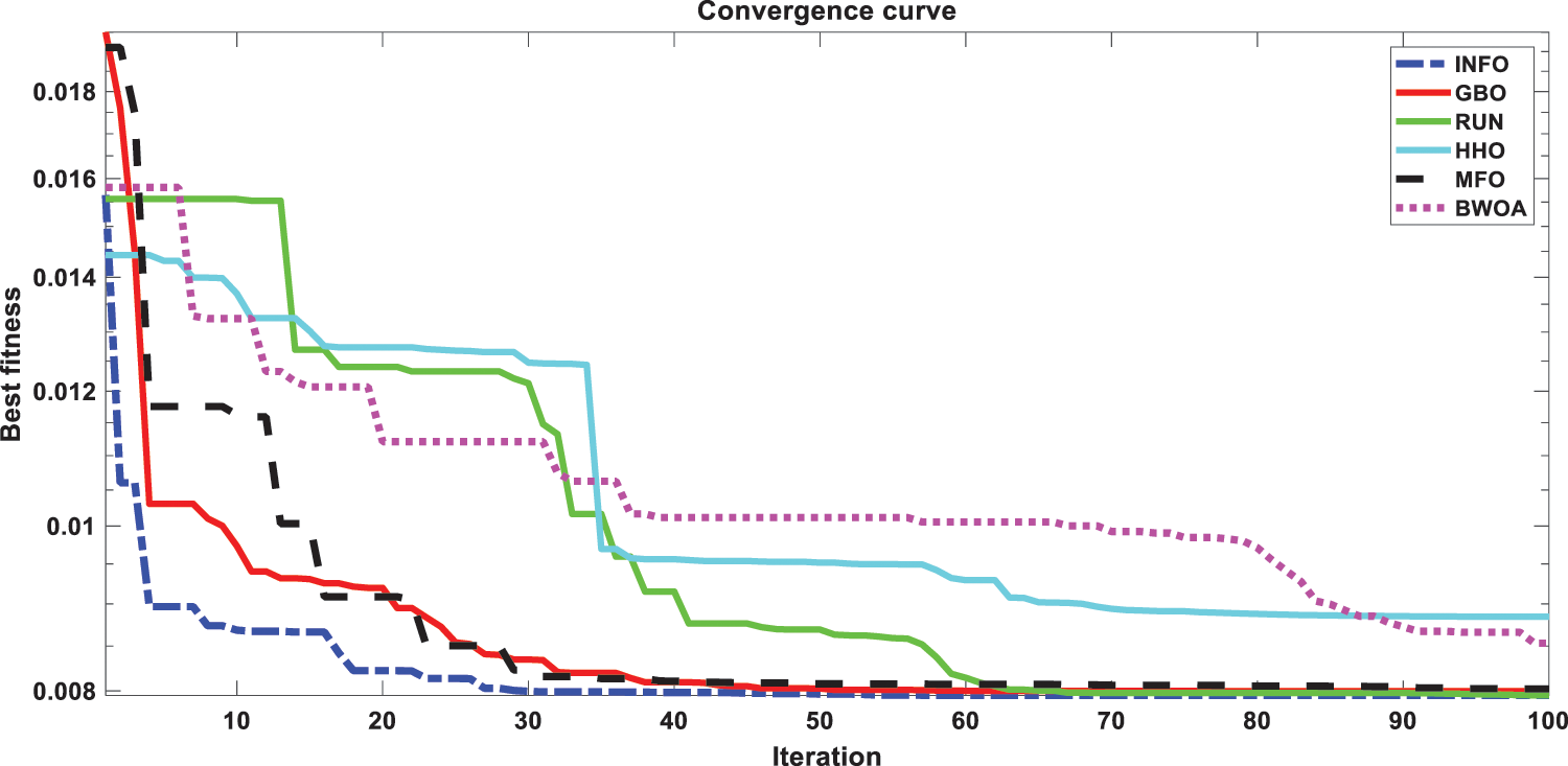
Figure 14: Convergence curves of various investigated algorithms for FOM

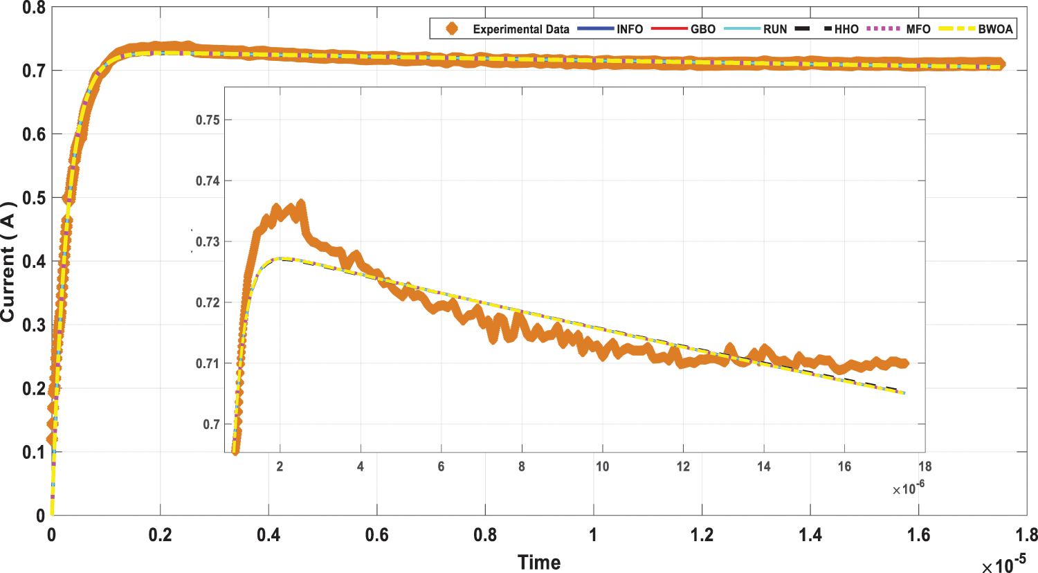
Figure 15: Load current curve for measured data and computed IOM by all investigated algorithms

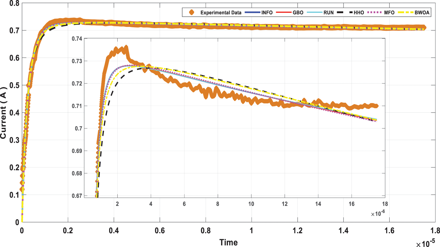
Figure 16: Load current curve for measured data and computed FOM by all investigated algorithms

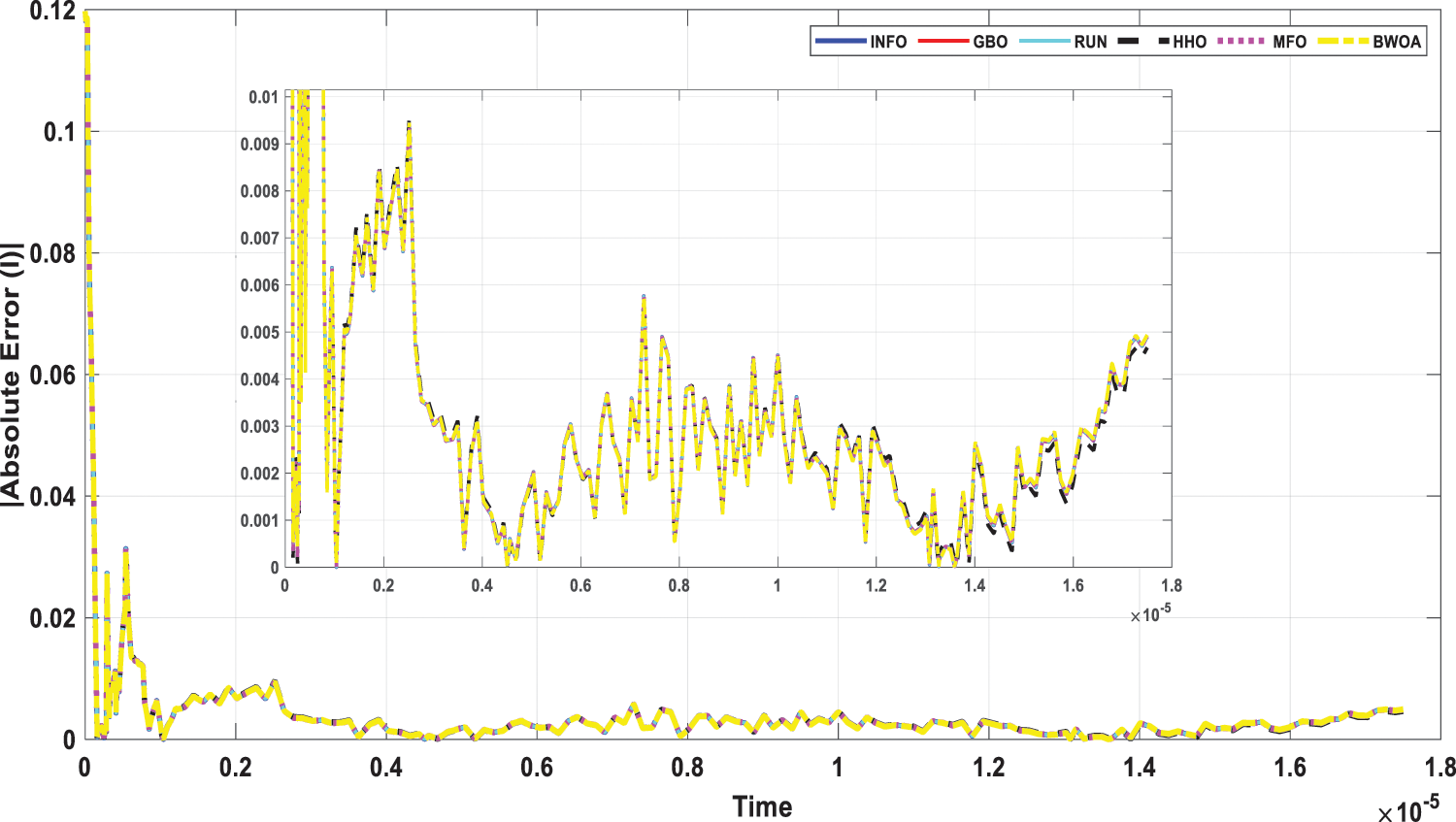
Figure 17: Current absolute error for computed IOM through all studied algorithms

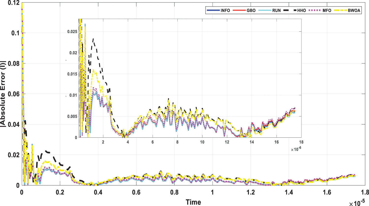
Figure 18: Current absolute error for computed FOM through all studied algorithms

5  Conclusion

This paper offered a new application of the INFO algorithm to precisely and rapidly estimate and identify parameters of static and dynamic PV models depending on experimental data sets. The parameters of both static models (SDM and DDM) were estimated using the INFO algorithm, which used measured data of RTC France’s merchant silicon solar cell with a diameter of 57 mm. Then, dynamic IOM and FOM models were estimated using the dataset, which was captured from the PV module at a temperature of 25°C with an irradiance level of 655 W/m2 through a connected load of RL = 23.1 Ω.

The extracted parameters’ purpose in both dynamic and static PV models was to minimize the root mean square error among the simulated and experimental currents of the merchant solar cell. The suggested INFO is a modern optimization technique used to minimize the objective function of photovoltaic parameter extraction and has several advantages, including faster convergence speed, solution accuracy, and balance. The outputs of the INFO algorithm were studied in a variety of ways to assess its performance. The algorithm’s accuracy was assessed by calculating the RMSE as well as the absolute error calculation, then comparing it with other algorithms. The flexibility and durability of the algorithms were verified by running them 50 times in a row, and the results were evaluated by statistical analysis. Through the results and analyzes, the proposed INFO algorithm has achieved more precise and robust results when compared with other contemporary algorithms. Thus, it’s a suitable option for tackling solar cell system optimization difficulties. In terms of future work, the INFO approach may be used to determine the PV parameters of any system, making it valuable for researchers and research investigations in the future.

Acknowledgement: The authors extend their appreciation to the Deputyship for Research & Innovation, Ministry of Education in Saudi Arabia, for funding this research work through the Project Number (IF-PSAU-2021/01/18921).

Funding Statement: This research is funded by Prince Sattam Bin Abdulaziz University, Grant Number IF-PSAU-2021/01/18921.

Conflicts of Interest: The authors declare that they have no conflicts of interest to report regarding the present study.

References

1. J. Jurasz, F. A. Canales, A. Kies, M. Guezgouz and A. Beluco, “A review on the complementarity of renewable energy sources: Concept, metrics, application and future research directions,” Solar Energy, vol. 195, pp. 703–724, 2020. [Google Scholar]
2. H. Sun, R. U. Awan, M. A. Nawaz, M. Mohsin, A. K. Rasheed et al., “Assessing the socio-economic viability of solar commercialization and electrification in south asian countries,” Environment, Development and Sustainability, vol. 23, no. 7, pp. 9875–9897, 2021. [Google Scholar]
3. O. A. Al-Shahri, F. B. Ismail, M. A. Hannan, M. S. H. Lipu, A. Q. Al-Shetwi et al., “Solar photovoltaic energy optimization methods, challenges and issues: A comprehensive review,” Journal of Cleaner Production, vol. 284, pp. 125465, 2021. [Google Scholar]
4. S. Lidaighbi, M. Elyaqouti, K. Assalaou, D. ben Hmamou, D. Saadaoui et al., “Parameter estimation of photovoltaic modules using analytical and numerical/iterative approaches: A comparative study,” Materials Today: Proceedings, vol. 52, pp. 1–6, 2022. [Google Scholar]
5. N. Araújo, F. J. P. Sousa and F. B. Costa, “Equivalent models for photovoltaic cell–a review,” Revista de Engenharia Térmica, vol. 19, no. 2, pp. 77–98, 2020. [Google Scholar]
6. H. Rezk, T. S. Babu, M. Al-Dhaifallah and H. A. Ziedan, “A robust parameter estimation approach based on stochastic fractal search optimization algorithm applied to solar PV parameters,” Energy Reports, vol. 7, pp. 620–640, 2021. [Google Scholar]
7. A. Sharma, A. Sharma, M. Averbukh, V. Jately and B. Azzopardi, “An effective method for parameter estimation of a solar cell,” Electronics, vol. 10, no. 3, pp. 312, 2021. [Google Scholar]
8. S. Wang, Y. Yu and W. Hu, “Static and dynamic solar photovoltaic models’ parameters estimation using hybrid rao optimization algorithm,” Journal of Cleaner Production, vol. 315, pp. 128080, 2021. [Google Scholar]
9. S. Lidaighbi, M. Elyaqouti, D. ben Hmamou, D. Saadaoui, K. Assalaou et al., “A new hybrid method to estimate the single-diode model parameters of solar photovoltaic panel,” Energy Conversion and Management: X, vol. 15, pp. 100234, 2022. [Google Scholar]
10. R. Ben Messaoud, “Extraction of uncertain parameters of double-diode model of a photovoltaic panel using ant lion optimization,” SN Applied Sciences, vol. 2, no. 2, pp. 1–8, 2020. [Google Scholar]
11. S. B. Prakash, G. Singh and S. Singh, “Modelling and performance analysis of simplified two-diode model of photo-voltaic cells,” Frontiers in Physics, vol. 9, pp. 236, 2021. [Google Scholar]
12. E. H. Houssein, G. N. Zaki, A. A. Z. Diab and E. M. G. Younis, “An efficient manta ray foraging optimization algorithm for parameter extraction of three-diode photovoltaic model,” Computers & Electrical Engineering, vol. 94, pp. 107304, 2021. [Google Scholar]
13. A. S. Bayoumi, R. A. El-Sehiemy, K. Mahmoud, M. Lehtonen and M. M. F. Darwish, “Assessment of an improved three-diode against modified two-diode patterns of MCS solar cells associated with soft parameter estimation paradigms,” Applied Sciences, vol. 11, no. 3, 2021. [Google Scholar]
14. M. Abdel-Basset, R. Mohamed, S. Mirjalili, R. K. Chakrabortty and M. J. Ryan, “Solar photovoltaic parameter estimation using an improved equilibrium optimizer,” Solar Energy, vol. 209, pp. 694–708, 2020. [Google Scholar]
15. I. A. Ibrahim, M. J. Hossain, B. C. Duck and M. Nadarajah, “An improved wind driven optimization algorithm for parameters identification of a triple-diode photovoltaic cell model,” Energy Conversion and Management, vol. 213, pp. 112872, 2020. [Google Scholar]
16. D. Yousri, D. Allam, M. B. Eteiba and P. N. Suganthan, “Static and dynamic photovoltaic models’ parameters identification using chaotic heterogeneous comprehensive learning particle swarm optimizer variants,” Energy Conversion and Management, vol. 182, pp. 546–563, 2019. [Google Scholar]
17. S. Mirjalili, “Moth-flame optimization algorithm: A novel nature-inspired heuristic paradigm,” Knowledge-Based Systems, vol. 89, pp. 228–249, 2015. [Google Scholar]
18. D. Kler, P. Sharma, A. Banerjee, K. P. S. Rana and V. Kumar, “PV cell and module efficient parameters estimation using evaporation rate based water cycle algorithm,” Swarm and Evolutionary Computation, vol. 35, pp. 93–110, 2017. [Google Scholar]
19. P. J. Gnetchejo, S. N. Essiane, P. Ele, R. Wamkeue, D. M. Wapet et al., “Enhanced vibrating particles system algorithm for parameters estimation of photovoltaic system,” Journal of Power and Energy Engineering, vol. 7, no. 8, pp. 1, 2019. [Google Scholar]
20. H. Chen, S. Jiao, M. Wang, A. A. Heidari and X. Zhao, “Parameters identification of photovoltaic cells and modules using diversification-enriched harris hawks optimization with chaotic drifts,” Journal of Cleaner Production, vol. 244, pp. 118778, 2020. [Google Scholar]
21. H. M. Hasanien, “Shuffled frog leaping algorithm for photovoltaic model identification,” IEEE Transactions on Sustainable Energy, vol. 6, no. 2, pp. 509–515, 2015. [Google Scholar]
22. D. H. Wolpert and W. G. Macready, “No free lunch theorems for optimization,” IEEE Transactions on Evolutionary Computation, vol. 1, no. 1, pp. 67–82, 1997. [Google Scholar]
23. A. Y. Hassan, A. A. K. Ismaeel, M. Said, R. M. Ghoniem, S. Deb et al., “Evaluation of weighted mean of vectors algorithm for identification of solar cell parameters,” Processes, vol. 10, no. 6, pp. 1072, 2022. [Google Scholar]
24. I. Ahmadianfar, A. A. Heidari, S. Noshadian, H. Chen and A. H. Gandomi, “INFO: An efficient optimization algorithm based on weighted mean of vectors,” Expert Systems with Applications, vol. 195, pp. 116516, 2022. [Google Scholar]
25. M. Premkumar, P. Jangir, C. Ramakrishnan, G. Nalinipriya, H. H. Alhelou et al., “Identification of solar photovoltaic model parameters using an improved gradient-based optimization algorithm with chaotic drifts,” IEEE Access, vol. 9, pp. 62347–62379, 2021. [Google Scholar]
26. A. A. Teyabeen, N. B. Elhatmi, A. A. Essnid and A. E. Jwaid, “Parameters estimation of solar PV modules based on single-diode model,” in 2020 11th Int. Renewable Energy Congress (IREC) IEEE, Hammamet, Tunisia, pp. 1–6, 2020. [Google Scholar]
27. Q. Hao, Z. Zhou, Z. Wei and G. Chen, “Parameters identification of photovoltaic models using a multi-strategy success-history-based adaptive differential evolution,” IEEE Access, vol. 8, pp. 35979–35994, 2020. [Google Scholar]
28. A. A. Z. Diab, H. M. Sultan, T. D. Do, O. M. Kamel and M. A. Mossa, “Coyote optimization algorithm for parameters estimation of various models of solar cells and PV modules,” IEEE Access, vol. 8, pp. 111102–111140, 2020. [Google Scholar]
29. A. Ramadan, S. Kamel, M. H. Hassan, T. Khurshaid and C. Rahmann, “An improved bald eagle search algorithm for parameter estimation of different photovoltaic models,” Processes, vol. 9, no. 7, pp. 1127, 2021. [Google Scholar]
30. I. Ahmadianfar, O. Bozorg-Haddad and X. Chu, “Gradient-based optimizer: A new metaheuristic optimization algorithm,” Information Sciences, vol. 540, pp. 131–159, 2020. [Google Scholar]
31. I. Ahmadianfar, A. A. Heidari, A. H. Gandomi, X. Chu and H. Chen, “RUN beyond the metaphor: An efficient optimization algorithm based on runge kutta method,” Expert Systems with Applications, vol. 181, pp. 115079, 2021. [Google Scholar]
32. A. A. Heidari, S. Mirjalili, H. Faris, I. Aljarah, M. Mafarja et al., “Harris hawks optimization: Algorithm and applications,” Future Generation Computer Systems, vol. 97, pp. 849–872, 2019. [Google Scholar]
33. A. F. Peña-Delgado, H. Peraza-Vázquez, J. H. Almazán-Covarrubias, N. Torres Cruz, P. M. García-Vite et al., “A novel bio-inspired algorithm applied to selective harmonic elimination in a three-phase eleven-level inverter,” Mathematical Problems in Engineering, vol. 2020, pp. 8856040, 2020. [Google Scholar]
34. M. C. Di Piazza, M. Luna and G. Vitale, “Dynamic PV model parameter identification by least-squares regression,” IEEE Journal of Photovoltaics, vol. 3, no. 2, pp. 799–806, 2013. [Google Scholar]
Cite This Article
Copyright © 2023 The Author(s). Published by Tech Science Press.
This work is licensed under a Creative Commons Attribution 4.0 International License , which permits unrestricted use, distribution, and reproduction in any medium, provided the original work is properly cited.
Downloads
Citation Tools