Generating Time-Series Data Using Generative Adversarial Networks for Mobility Demand Prediction

1  Introduction

The electric vehicles (EVs) have generally become a necessary means of increasing energy efficiency and lowering emissions. The global mobility sector is undergoing significant changes because of connectivity, autonomous driving, and shared mobility advancements. Many countries have made it a priority to achieve sustainable transportation to meet future energy demands. Electric kickboards and scooters are anticipated to become more popular over time as a result of the rising demand for fuel-efficient automobiles brought on by growing worries over greenhouse gas and carbon emissions. EVs are critical in improving energy security and reducing greenhouse gas and other pollutant emissions. EVs are a comfortable transport system, which is much more in demand now. Electric vehicles are an advantageous eco-friendly mode of travel, positively contributing to reducing air pollution, parking demand, and traffic congestion. E-kickboards are becoming increasingly popular, especially in tourist areas of the world, properly deploying electric kickboards rental system and location that customers desire is crucial for maintaining a competitive edge and offering top-notch customer service. The free-floating service has the benefit of providing pick-up and drop-off anywhere. Still, as it is dispersed around the service area, it has the drawback of being unavailable at the desired time and location. Unavailability of EVs due to restrictions, customers could be unsatisfied with the service, and if the company continues this situation, demand could drop, and sales could suffer [1]. Forecasting is the process of predicting a product or service’s future requirements. Accurately anticipating customer needs in the mobility industry’s data-driven business environment is a critical success. There are well-known machine learning algorithms to forecast demand for electric kickboards, although the prediction error rates are frequently large. Even if the expected demand value and the actual demand value are off by a few percentage points, there could still be a significant financial loss. Based on this idea, we have divided the area on Jeju Island into various places according to the centroid. Nearby rental stations were specified and quickly relocated to the faults where the kickboard needed to improve the electric kickboard demand prediction. When the demand in a specific area is higher than the forecast for that area, the electric kickboard can be brought to the center of that area and provide timely service.

The vehicle movement between stations is one of the main problems system operators faces and needs to be solved urgently based on accurate estimates of station demand [2]. Electric vehicles (EVs) are considered the most viable technology option for decarbonizing passenger transport globally, especially when combined with a low-carbon energy system [3]. We need to deploy the prediction system to predict kickboard demand for eliminating financial loss and increasing business. Initially, the forecast error rate is high because actual data contains fewer records for a specific region. The rent_number is minimal because there are fewer records on some particular days for various reasons. The necessary step will be the evenness of record variation to accurately predict customer demand, which can be accomplished by generating new data with a lower frequency to reduce prediction error. Data scarcity can be addressed by synthetic data generation. Artificially generated data duplicating the original data’s statistical properties is known as synthetic data. In developing synthetic data, several concepts related to Machine learning (ML) were applied. In this paper, we use generative adversarial networks to generate synthetic new time-series data, which is later combined with the original data to reduce prediction error and enhance accuracy. The main takeaways of our proposed work are the following:

•   We proposed a synthetic time-series data generation technique using the GAN approach.

•   The proposed GAN model is TGAN-Modified-WGAN-GP, a tabular generative adversarial networks (TGAN) architecture for training with TGAN to produce synthetic time-series data that evolved from a modified version of Wasserstein GAN with gradient penalty (WGAN-GP), which improved training stability, made it more robust to mode collapse problems, and made convergence faster.

•   We integrate k-means clustering to extract region-based data and a stacking technique-based blending ensemble to create a prediction model for mobility demand.

•   A detailed comparative study with the existing baseline ML models and different ensemble models.

Utilizing electric kickboard data from a service provider that started operating on Jeju Island in April of this year, the study examined demand predictions. Several ways for improving the predictive performance of regression ensemble models for demand forecasting have been documented in the literature. Raju et al. [4] tested their stacked-based ensemble technique on the steel industry dataset and discovered that it enhances model performance and minimizes decision-making risk. One month ahead of time, the ensemble approach can forecast demand in the steel industry. Historical data for projecting power demand considers the charging demand of EVs parking lots. The process is based on the auto-regressive integrated moving average (ARIMA) model. The proposed approach by Amini et al. reference [5] enhances predicting accuracy. The projected load for each parking lot’ daily charging demand is estimated using probabilistic hierarchical EVs parking lot demand modeling. The proposed approach is tested on Pennsylvania, New Jersey, and Maryland (PJM) is a regional transmission organization (RTO) that coordinates the movement of wholesale electricity historical load data to determine its efficacy. The simulation results reveal that the proposed strategy for anticipating electricity demand is accurate. A deep learning (DL) framework was presented by [6] to forecast taxi-passenger demand while simultaneously considering geographical, temporal, and external relationships. The suggested DL framework coupled a modified density-based spatial clustering technique with noise (DBSCAN) and a conditional generative adversarial network (CGAN) model. The updated DBSCAN model was used to create sub-networks that considered the spatial correlation of taxi pick-up events in the road network.

The method of using mutual variations to enhance grouping and area forecasting was proposed and investigated in the publication by Zhang et al. [7]. First, a taxi zone grouping algorithm has been created that takes into account the relationships between the various taxi zones and is based on the notion of grouping in pairs. Since then, internal and intercluster features have been achieved, respectively, through the development of group-level and global prediction modules. In order to merge the two modules, a multi-level recurrent neural network model is suggested.

Two important points are made in the article by Cao et al. [8]: taxi demand vary significantly between functional regions, and taxi demand follows a dynamic daily and weekly pattern. We use Points of Interest (POIs) to identify regional functions and present a unique bidirectional encoder representation from transformer (BERT)-based Deep Spatial-Temporal Network (BDSTN) to model complex spatial-temporal interactions from heterogeneous local and global information to address these two difficulties. To their knowledge, this is both the first time they have thought about the practical parallels and the first time proposed architecture has been utilized to identify the different types of taxi claims. The recommended method applies more complex procedures, and their suggested model is significantly superior than previous ways, according to their research findings using the New York City Real Traffic Database. A cutting-edge deep neural network is improved to anticipate electric vehicle charging needs with a 15-minute temporal resolution for the day ahead. New elements have been introduced by [9], the neural network to enhance EVs charging predicting. The forecaster is used on a critical use case of a hospital’s local charging site. The results show that their approach reduced error to estimate a high stochastic aggregated EVs charging demand on a day-ahead horizon with a mean absolute error (MAE) less than 1 kilowatt (kW) is the research’s key accomplishment. The study by [10] proposed to forecast building energy usage, and they devised a stacking model. This model combines the benefits of numerous base prediction methods and creates meta-features to determine the dataset’s spatial and structural angle. Rezagholiradeh et al. [11] used GAN to solve the regression problem. In this process, the GAN structure generates train data and does forecasting. This system is successful in decreasing the suggested model’s mistakes. The article by Tian et al. [12] proposed a similar technique for producing artificial data based on GAN that uses only a small quantity of data. The applied dataset contains original and generated data using ML forecasting models. Zhang et al. [13] provided stock market forecasting using GAN based on the long short-term memory (LSTM) and Multi-Layer Perceptron ML models in their article. The train set contains daily stock data, and this procedure demonstrates how this system’s predicting accuracy has improved. A model that generates synthetic data using a generative adversarial network uses time-series energy consumption data as input to an expansion technique and then combines it with the original data to reduce the energy consumption prediction error [14]. Their proposed TGAN-Skip-Improved-WGAN-GP model converges faster than existing GAN models for synthetic data generation. The experimental results show that mixing synthetic data and real data can significantly reduce the prediction error rate and improve the accuracy of energy consumption prediction. The parameters of the LSTM network are optimized using the whale optimization algorithm, which uses adaptive particle swarm optimization to correctly forecast the bandwidth of the metamaterial antenna [15]. Using the community structure method, five communities were formed within the region. Kim et al. [16] created an LSTM-based hourly demand forecast model; they used hyperbolic tangent and exponential linear unit to achieve accurate predictions. A deep learning model-based solution for relocating and utilizing taxi data is developed to determine the best service system. The suggested strategy can significantly lower operating costs and on-demand service times [17]. Yi et al. [18] proposed a model for electric vehicle demand prediction that acquired acceptable accuracy. In [19], by applying random forest-based demand prediction in Germany to understand ride-pooling trip origins and spatial characteristics in two cities.

2  Proposed Methodology

In this study, we described our proposed approach to how synthetic time series data generated using generative adversarial networks could affect to reduce prediction error. When training a ML model using synthetic data combined with original data, the prediction error rate is much lower than that using only original data. Our proposed work is divided into two cases depicted in Fig. 1. As input, we considered electric kickboard data from a local kickboard company in Jeju Island, South Korea. In the first case, data is preprocessed to predict the demand, then we used k means for region-based clusters and the blending ensemble regressor model for the final demand prediction. In the second case, the original data is fed into the GAN model to generate realistic synthetic data that has the same data distribution as the original data using our proposed GAN model. After that, generated synthetic data will be preprocessed before stepping into the further stage. The actual data is merged with synthetic data for further evaluation. The prediction error is then evaluated with original data and original data combined with the synthetic data. The quality of generated synthetic data by our proposed model is assessed in the results section and compared with other models that generated synthetic data.

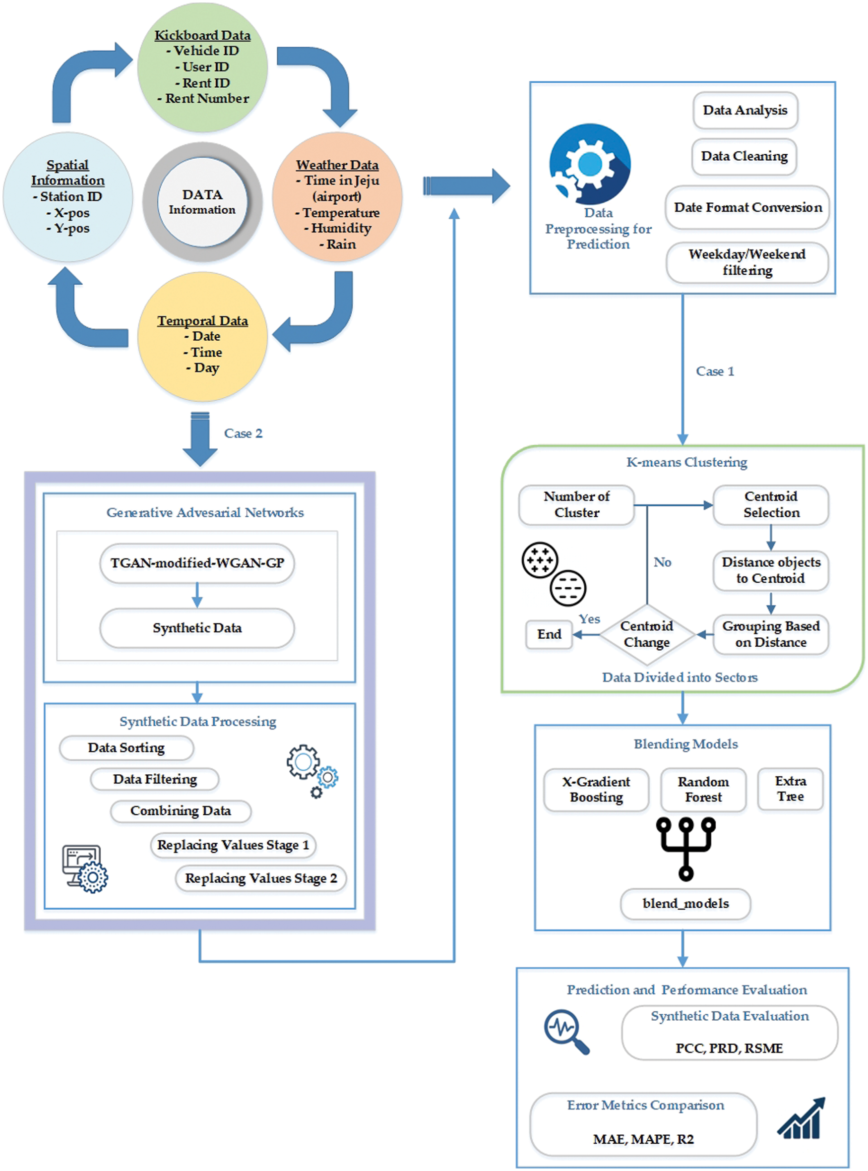
Figure 1: Overview of the proposed architecture of demand prediction

2.1 Dataset

This section will overview the data we used in our experiment. We have collected the data from a local EVs service provider in Jeju Island, South Korea. Its main task is to determine daily kickboard requirements based on various parameters, generate synthetic data using a GAN model, and solve the problem of dataset imbalance and minority data oversampling. The dataset contains information from April 2019 to June 2021, and we have got kickboard, spatial, and temporal data from the company. The another important weather information collected from the Korean metrological department. The Kickboard data holds vehicle_id, user_id, rent_id, and rent_number. Therefore, for every category, data have different data specifications. The Spatial data holds information about station_id, x_pos, and y_pos, whereas Temporal data contains information on the day, date, and time. The raw weather data has time, temperature, humidity, and rain information. Fig. 1 shows the data information used in our experiment. The data we obtained for research holds 717 days of rent data from the year 2019 to 2021. The daily demand for electric mobility data is gathered in the system of the rental service provider. The environment significantly impacts every business if it is based on a transpotation system. For that reason, we imported weather data from the Korea Meteorological Administration. We divided weekends from weekdays and incorporated external variables that influence the use of electric mobility, such as daily average temperatures and precipitation. The daily demand for electric kickboards both before and after smoothing is shown in Fig. 2. The date is represented on the x-axis, while the total daily demand for that day is shown on the y-axis. As a fledgling business, this can be viewed as a demand that was modest at first for service but picked up after a while. The need also changed significantly from day to day and was not constant. These unsteady data were smoothed in order to undertake this investigation. The window size for data smoothing was set to 11, and this size groups the day with the days before and after it to normalize the data. The midday and the five days before and after are included in the 11-day timeframe.

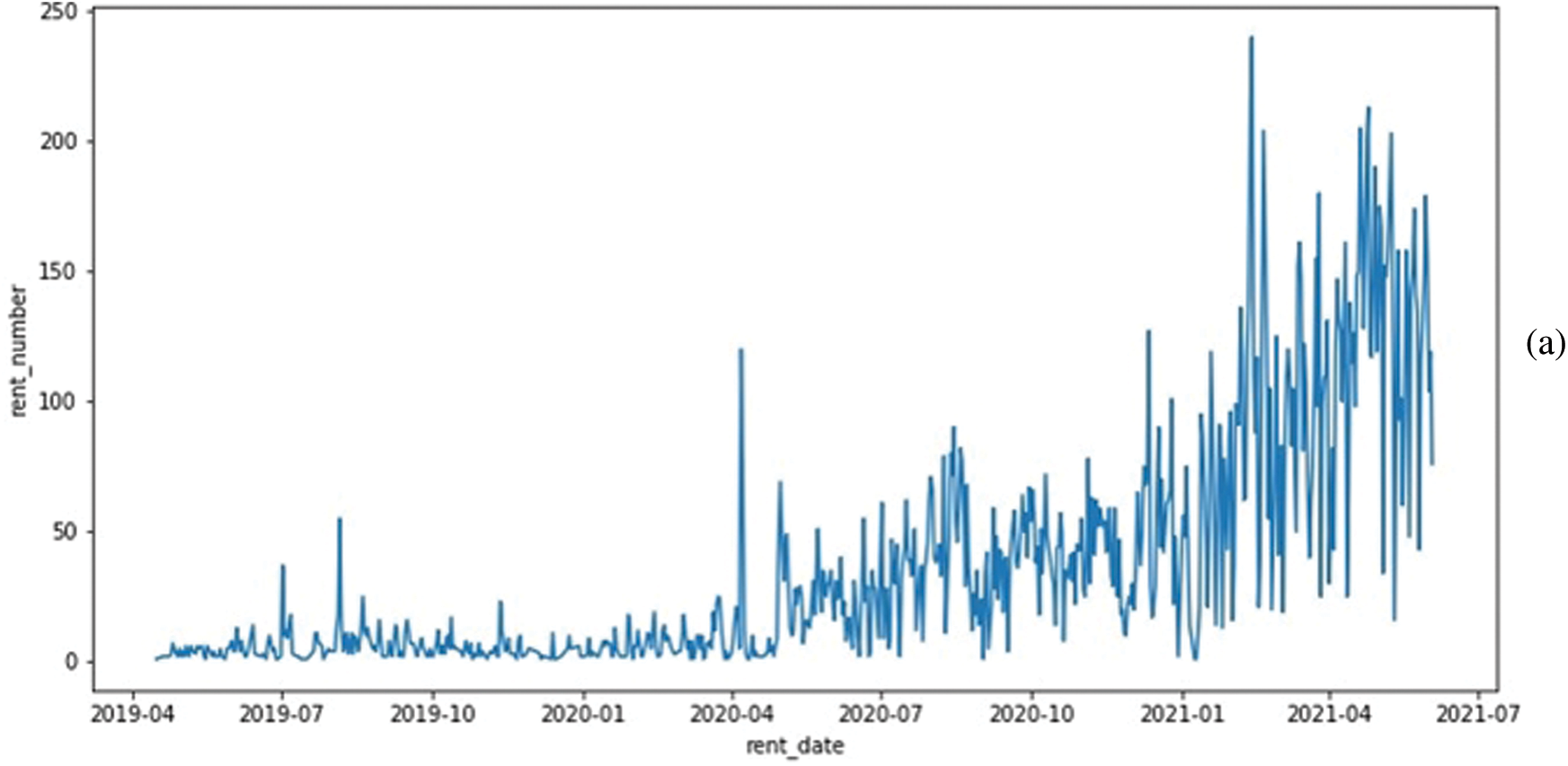
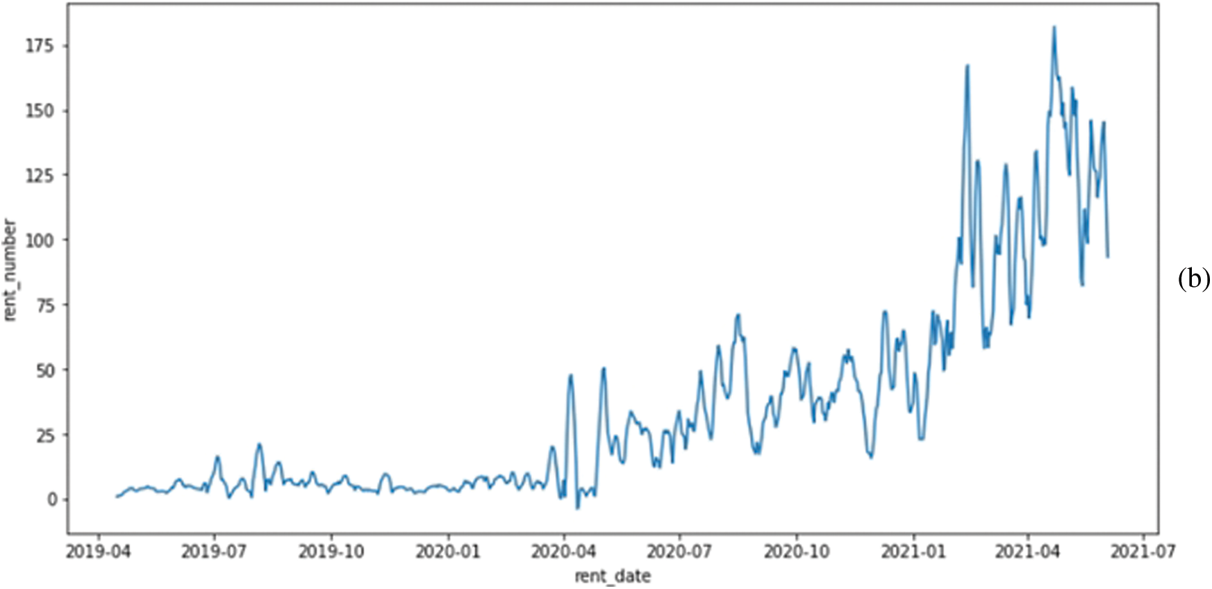
Figure 2: (a) Plot of daily demand before smoothing and (b) Plot of daily demand after smoothing

2.2 Data Preprocessing for Prediction

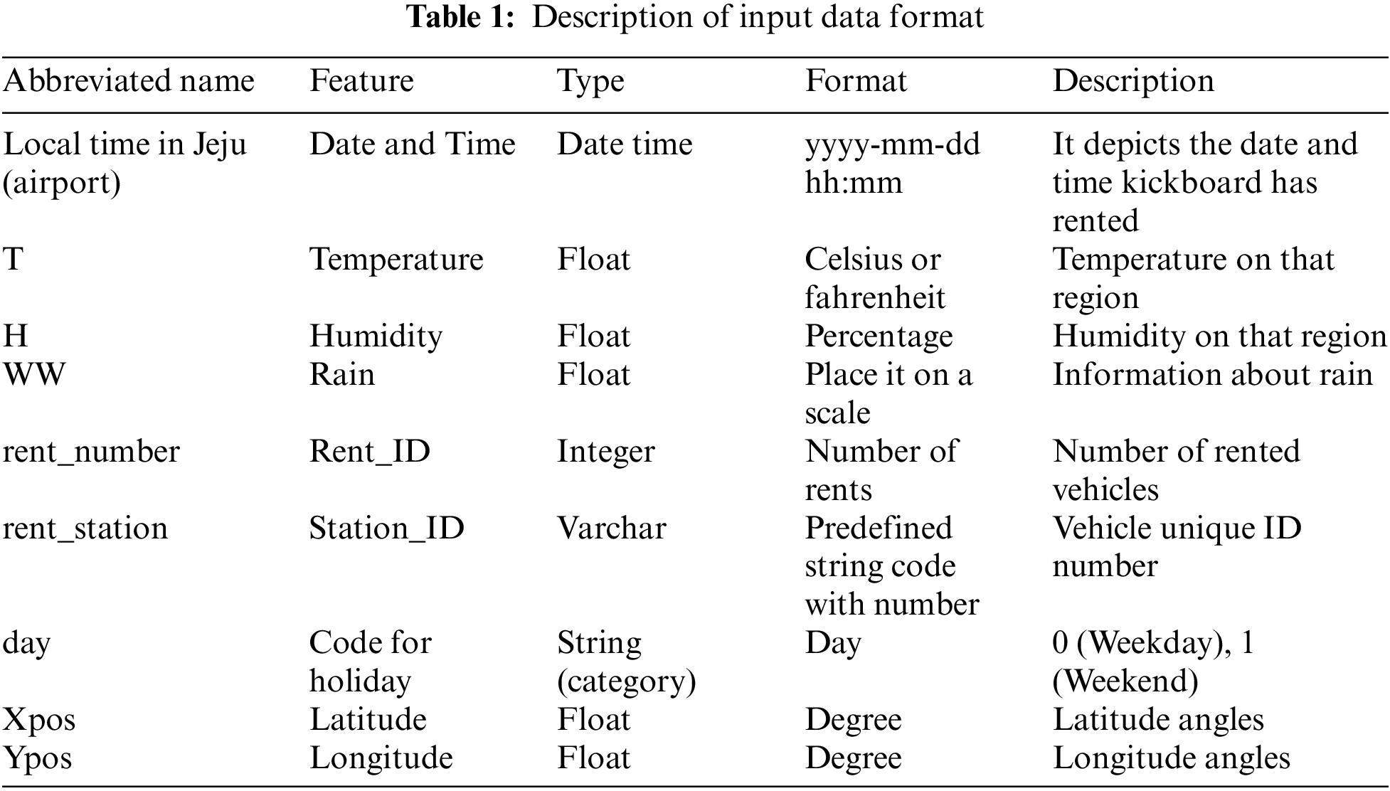
The collected data has four CSV file formats of different sources and information; Kickboard, spatial, temporal, and weather data are used to investigate the impact of various parameters on our demand prediction. Original datasets obtained from the company contain multiple characteristics. The characteristics were selected based on their importance and application in forecasting kickboard demand. Several processes were involved in the data preprocessing. Later, the data were minutely combined to build the final dataset. We have selected 13 features employed for our experiment, where T represents temperature, I describe insulation, and H means humidity. Sector0 is the first sector, and sector3 is the 4th sector. Other features are day, month, year, weekend, rain, and holiday. We have noticed that the temperature, insulation, and humidity significantly impact the final prediction. Date format conversion includes formatting the rent_date column value into the year, month, and day format. Later preprocessing on the day when weekdays and weekends are filtered; Saturday and Sunday have considered holidays. Multiple strategies are used to preprocess this data. Outlier removal and feature extraction are two examples of the data cleaning process. Several ML packages were imported to at the beginning of our experiment, including NumPy, pandas, pycaret, and seaborn. The dataset sample used in this study is shown in Table 1.

2.3 Generative Adversarial Networks for Generating Synthetic Data

2.3.1 Overview of Traditional GAN Framework

Unsupervised learning models that incorporate supervised loss as part of their training are known as GAN, introduced by Goodfellow et al. [20]. Two networks are competing in a min-max game. The first is the generator that has been trained to generate new samples, and the second is the discriminator that determines if the input sample is real or fake. As shown in Fig. 3, the generator (G) is a transformation-based neural network. This generator accepts a random noise pnv(nv) from which it tries to retain data distribution pdata over data x. After the generator has been trained, the discriminator is fed with the samples generated by the generator network. The Discriminator network accepts two inputs: the data produced by the generator and the other is actual data. Further, the discriminator network is trained on a real sequence and performs the task of classifying the data produced by the generator to be real or fake.

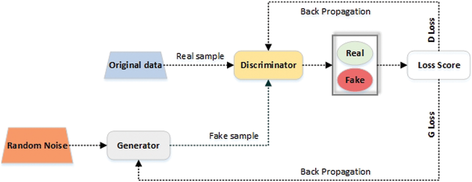
Figure 3: Simple architecture of the generative adversarial networks

The discriminator (D) is based upon a different neural architecture and acts as a discriminative function. The discriminator seeks to increase the performance of the generator until the samples generated by it can no longer be distinguished from real data. The generator G plays with log(1−D(G(nv))) to minimize the objective function such that D(G(nv)) is close to 1 (a false generated data is detected as true by the discriminator). The loss function is defined as Eq. (1).

minGmaxDL(D,G)=Ex∼pdata (x)[log⁡D(x)]+Env∼pnv(nv)[log⁡(1−D(G(nv)))](1)

In binary classification issues, L(G, D) is a binary cross-entropy function is often utilized. Both G and D backpropagate the loss function in the Eq. (1) through their respective models to update the parameters.

2.3.2 TGAN-Modified-WGAN-GP

The original TGAN architecture uses the vanilla GAN training, except for an additional KL-divergence term in the loss of the generator. Xu et al. [21] suggested the TGAN architecture in Fig. 4 for tabular data creation. The authors wanted to create a tool to generate datasets containing categorical or continuous data. This is done using a recurrent neural network (RNN) with a LSTM cell intersecting a column and predicting the next column’s value based on the previous output. The output of the LSTM goes through several dense layers, including the attention layer, to get the outcome. The discriminator is much simpler and consists only of a fully connected network. It can also identify neural network problems when dealing with inputs with non-gaussian distributions and provide random distribution strategies to solve them. Use a gaussian mixture model (GMM) applied to each numeric column individually. This method is called the normalization of numerical variable patterns. Introduced a GAN model with Gradient Penalty that blends Tabular GAN (TGAN) and modified Wasserstein GAN architectures with gradient penalty (WGAN-GP). We present Modified-WGAN-GP architecture with SN to smoothen the loss function. The RMSprop optimizer was employed instead of the Adam optimizer in both G and D. SN guarantees that the discriminator (D) is K-Lipschitz continuous. It acts on each layer of the critic to bind the Lipschitz constant. The generated synthetic time series data using the proposed model significantly reduces the prediction error rate when used for prediction. The TGAN-Modified-WGAN-GP model processes the data to generate the final synthetic data.

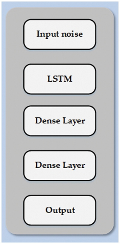
Figure 4: TGAN architecture

Gulrajani et al. [22] proposed an enhanced version of Wasserstein’s GAN (Arjovsky et al. [23]) that adopts a gradient penalty (GP) approach instead of weight clipping that can cause capacity problems and requires additional parameters to define the weights’ space. It presents a GP that satisfies the 1-Lipschitz condition without requiring clipping. The gradient penalty is increased or decreased by WGAN-GP depending on how far the gradient is from being 1-Lipschitz. We used the following objective function in Eq. (2), where a new loss is represented as the original Wasserstein loss by the first two terms, while the last term means the gradient penalty term.

Loss =Ex¯∼Gdata [D(x~)]−Ex∼Prv[D(G(x))]+λEx^∼Vx^[(||∇x^D(x^)||2−1)2](2)

where Prv and Gdata represent data and generator distribution on random samples, x^∼Vx^.λ is set to 10 according to [24] on our experiment. It worked well with various datasets and architectures.

WGAN-GP architecture for generating univariate synthetic time-series data. The proposed architecture is a mix of G and D linear and convolutional layers that work by default. Unfortunately, training is not stable in the default setting where batch normalization (BN) is used. So, we removed BN and used Miyato et al. [25] proposed Spectral Normalization (SN). Simply put, SN guarantees that D is K-Lipschitz continuous. To this end, we are gradually working on critic layers that limit the Lipschitz constant. Nonetheless, SN improves training stability and accelerates convergence thus we modified the batch normalization to SN in both the generator and the discriminator. Finally, the original WGAN-GP recommended Adam optimizer for G and D but we removed the Adam optimizer and replaced it with RMSprop that will better our needs. This study is the first for the one-dimensional layer use of Wasserstein’s GAN with gradient penalty coupled with 1-dimensional convolutional networks to work on time series data. We employed noise data at first and then up sampling 1-dimensional for up sampling it and a dense layer to generate the samples by the generator. In the discriminator, 1-dimensional convolutional networks played the part with three dense layers that hold the critic architecture. We utilize RMSprop as the optimizer for training, using a base learning rate of η = 0.00005.

Mode collapse should be less likely when the Wasserstein distance is used. Overall, the model should converge to the optimum smoother and faster than vanilla GAN and perform better. While WGAN-GP is a minor change in concept, it necessitates some significant code changes. The gradient penalty must first be determined, and the loss function fitted to the Wasserstein distance. The discriminator’s spectral normalization must be adjusted for layer normalization. The training ratio between the generator and discriminator must be changed, and we train the discriminator in more iterations than the generator in WGAN-GP.

2.4 Synthetic Data Processing

The synthetic data processing step performs various operations, including sorting, filtering, amalgamating data, replacing values in stage 1, and replacing values in stage 2. After generating synthetic time-series data by our proposed model, it must be preprocessed before adding up with the original data. They are first constraining the data of the GAN generation rent_station IDs so that the GAN will not generate new rent_station IDs before training the GAN model. Then select the composite data with dates in the original data. The original and synthetic data are then merged. Sorting the data as per the rent_date is an important step. In replacing values in stage 1, we replaced the rent_number of the value 0 with 1, and in step 2, which replaced the negative value of rent_number with the absolute value.

2.5 K-means Clustering

The conventional k-means algorithm is briefly described in this section. In data mining, k-means is a standard unsupervised clustering algorithm frequently used to cluster large data sets. Hartigan et al. [26] 1979 proposed the k-means clustering algorithm. It is a partitioning clustering algorithm in which the input data objects are classified into k separate clusters by an iterative process that converges to a local minimum. As a result, the groups that are created are compact and self-contained. The algorithm is divided into two parts. The first phase picks k centers randomly, with the value k predetermined. The following step is to transport each data object to the nearest data center. The distance between each data object and the cluster centers is usually calculated using Euclidean distance [27]. Fig. 1 shows how k-means clustering work in the k-means clustering section. The dataset was created by preprocessing the data. A selected k-means clustering algorithm was applied to develop specified number of clusters. Considering the whole Jeju region as one and forecasting the overall demand, in this process we have created four clusters. The cluster number indicates a related or similar regional segment. The knowledge gained can be used for decision-making.

2.6 Regression Based Blend Model

PyCaret provides a blend_model function in the regression module. The PyCaret’s Python library provides this module. Mixture function for training a soft-voting classifier on the model specified by the estimator_list parameter. blend_models() is a method of ensembling that uses consensus among estimators to generate final predictions. Main advantage behind blending is to combine different ML algorithms and use a majority vote, or the average predicted probabilities in the case of regression. Blend_models() can be used with some pre-defined models, which you can pass using estimator_list. This function returns a scoring grid containing the results of the 5-fold cross-validation. Mixed-based soft voting is used to predict class labels based on the expected total probability argmax recommended for an ensemble of appropriately tuned classifiers. Regression analysis evaluates the association between one or more independent variables (often called “features,” “predictors,” or “covariates”) and dependent variables (sometimes called “outcome variables”). A set of statistical techniques is used in order. or “target” or “target variable”). In ML, the goal of regression is to predict continuous values. In our study, we have used PyCaret’s regression-based blend module for demand prediction. PyCaret’s Regression module (pycaret. regression) is a supervised ML module that uses various techniques and algorithms to predict continuous values/outcomes. Regression can predict values/outcomes such as sales, units sold, temperature, or any continuous number. PyCaret’s regression module has over 25 ready-to-use algorithms and 10 plots to analyze the performance of models. PyCaret’s regression module has it all: hyper-parameter tuning, ensembling, or advanced techniques like stacking. Blending-based soft voting predicts class labels based on argmax, the sum of predicted probabilities recommended for an ensemble of appropriately tuned classifiers. Among the latest ML models, extremely randomized trees, or (extra-trees) [28], random forest [RF] [29], and extreme gradient boosting (XGBoost) [30] have been gaining popularity in making predictions with the highest accuracy at a faster rate. In our work, we have passed blend function trains a voting regressors for select models given in the estimator_list param. Further, we have ensemble the abovementioned three models in the estimator_list for final prediction.

Instead of bagging, where each sample independently predicts the outcome, extreme gradient Boost reflects the weight of the result from the first sample to the succeeding sample. It continues to learn the weights of the results from the previous sample to affect the following sample. Compared to previous gradient boosting-based models, XGBoost offers a faster learning rate and superior model performance [31]. Gradient Boosting mainly focuses on the training data outcomes, which leads to overfitting very soon. By modifying the hyper parameter values supplied by the programmers and configuring the appropriate learning strategy, XGBoost can prevent overfitting. An open-source machine learning model called XGBoost supports regression and classification models and detects and fills in missing values in massive amounts of complex data. It works well to find the best tree model using other approximations without overfitting the data. External parameters (independent variables) have not been reported using the XGBoost algorithm to estimate demand. The ML models utilized in this research can enhance predictions and lower the margin of error between predicted and test data. ML has recently gained popularity in the field of mobile demand forecasting. For electric mobility service providers who wish to precisely forecast demand at a particular place in the city, the study’s findings may be useful. RF is an integrated learning strategy that combines numerous decision trees to remove feature data correlation [32]. By picking samples and features at random, RF reduces the correlation between decision trees. First, the same quantity of data from the training sample in the original training data is randomly selected. Second, a subset of the features is chosen randomly to create the decision tree. These two types of randomizations lessen the correlation between each decision tree, lowering the error that can occur when the decision tree is over-fitting and increasing the model’s accuracy.

An extremely randomized tree regressors can only be utilized in ensemble approaches. Extra tree regressors learns in a similar way to random forest [33]. The Extra Trees algorithm will randomly sample the features at each split point of a decision tree, similar to Random Forest. The Extra Trees algorithm chooses a split point at random in contrast to the random forest, which employs a greedy algorithm to choose an ideal split point. The training dataset is used to generate a large number of unpruned decision trees as part of the Extra Trees technique. In the case of regression, predictions are formed by averaging the results from the decision trees.

3  Result and Evaluation

This part includes a full review of the outcomes obtained through trials and a detailed performance analysis for demand forecasting. There are two sorts of research done on experimental results. First, we examined several current GAN models and offered performance comparisons with other GAN models on creating synthetic time series data using our suggested model. Second, the prediction outcomes of our blending regressors model are compared to typical ML models, emphasizing the importance of the suggested work.

3.1 Experimental Setup

Here, we will discuss the details of the system setup used to conduct our study. We have used the windows operating system with NVIDIA GeForce RTX 2070 GPU and 16GB of memory. We train our model on Tensorflow 2.6.0, CUDA Toolkit, 11.2, and cuDNN version 8.1. Jupyter usaed as IDE that runs on machine and python 3.7.11 as the programming language.

3.2 Evaluation Metrics of Synthetic Data

3.2.1 Pearson’s Correlation Coefficient

The Pearson R statistical test uses the Pearson correlation coefficient [34] to measure the strength between the different variables and their relationships; it ranges between −1 and 1. The ratio of oversampled raw to synthetic data is essential for evaluating synthetic data. A negative value indicates an entirely negative correlation between the variables. A positive value indicates a strong positive correlation. The higher the absolute value of the correlation coefficient, the stronger the correlation between variables. The Pearson’s correlation coefficient PCC in our proposed methodology was evaluated as Eq. (3), where Orig denotes the original data and Syn denotes the synthetic data. Number of sample size denoted by n, Syni and Origi are represents the individual sample points indexed with i. Orig¯ is mean of original data and, Syn¯ is mean of synthetic data.

PCC=∑i=1n(Origi−Orig)(Syni−Syn)[∑i=1n(Origi−Orig¯)][∑i=1n(Syni−Syn¯)](3)

3.2.2 Percent Root Mean Square Difference

The Percent Root Mean Square Difference (PRD) has been used to calculate the distortion between two signals between the original and the generated signals. It is defined as Eq. (4), where Orig depicts the original data and Syn depicts synthetic data.

PRD=100∑i=1n(Origi−Syni)2∑i=1n1(Origi)2(4)

3.2.3 Root Mean Square Error

The square root of Mean Squared Error (MSE) is Root Mean Squared Error (RMSE). MSE is a representation of how predicted values differ from actual values. Because errors might be positive or negative, we use the square root to prevent the negative sign. In Eq. (5), where YOrig depicts the original data and YSyn depicts synthetic data, following formula is used to represent it.

RMSE=n∑i=1n(YOrigi−YSyni)2(5)

3.2.4 Mean Absolute Error

The average difference between the observations (actual values) and model output is known as the mean absolute error (MAE) (predictions). MAE calculates the average absolute difference throughout the dataset to determine the difference between real and estimated values and the average error size. It is expressed as in the Eq. (6). Where actual depicts the actual value and pred depicts the predicted value.

MAE=1N∑iN|yi, actual −yi,pred|(6)

3.2.5 Mean Absolute Percentage Error

The Mean Absolute Percentage Error (MAPE) is a statistical measure of a ML algorithm’s accuracy on a given dataset. The error termed by the model evaluation can be defined by MAPE, which can be thought of as a loss function. We can measure the accuracy of the disparities between actual and estimated values using MAPE. MAPE can also be calculated as a percentage. The low MAPE indicates a reasonable accuracy rate for the prediction model. The formula for computing MAPE is found in Eq. (7). Where actual depicts the actual value and pred depicts the predicted value.

MAPE=100%n∑k=1n|(yactual−y^pred)yactual|(7)

3.2.6 R2 Score

The R2 score is critical for assessing a regression-based ML model’s performance. It is also known as the coefficient of determination and is commonly written as R squared. It operates by calculating the amount of variation in the dataset-explained predictions. Explained, it’s the difference between the dataset’s samples and the model’s predictions. R2 score is describe in Eq. (8). Where actual depicts the actual value and pred depicts the predicted value.

R2=1−∑(yactual−ypred)2∑(yactual−y¯pred)2(8)

For our experiments, CTGAN, TGAN, TGAN-Skip, LSTM-AE, TGAN-Skip-Improved-WGAN-GP, CWGAN-GP-PACGAN, TGAN-Skip-Improved-WGAN-GP, and TGAN-Modified-WGAN-GP (The resulting synthetic dataset was evaluated using the proposed similarity scoring method. The proposed model outperformed alternative models throughout the experiments, and recommendations were made. The metrics presented correlate well with sample quality, indicating that it is a good indicator of synthesizer performance. The LSTM cell utilized by TGAN has a hidden state length of 50 and an output feature-length of 64. Our discriminator contains one dense layer with 50 nodes and a learning rate of 0.001. Our random noise vector has a length of 200 and an L2-norm of 0.00001. These models were trained on the datasets for 700 epochs, with (N/batch size) as the number of steps and batch size = 200 as the number of rows. With our suggested TGAN–Modified-WGAN-GP model, we evaluated the quality of generated synthetic data with several existing GAN models depicted in Table 2. The results show that, in comparison to other current models, the synthetic data produced by TGAN-Modified-WGAN-GP is more correlated to the original data, indicating that our suggested model produces superior results and may be utilized to produce synthetic time-series data. As we can see from Table 2, our proposed model achieves a better result than existing models, with a correlation coefficient value of 0.947.

3.3 Demand Prediction

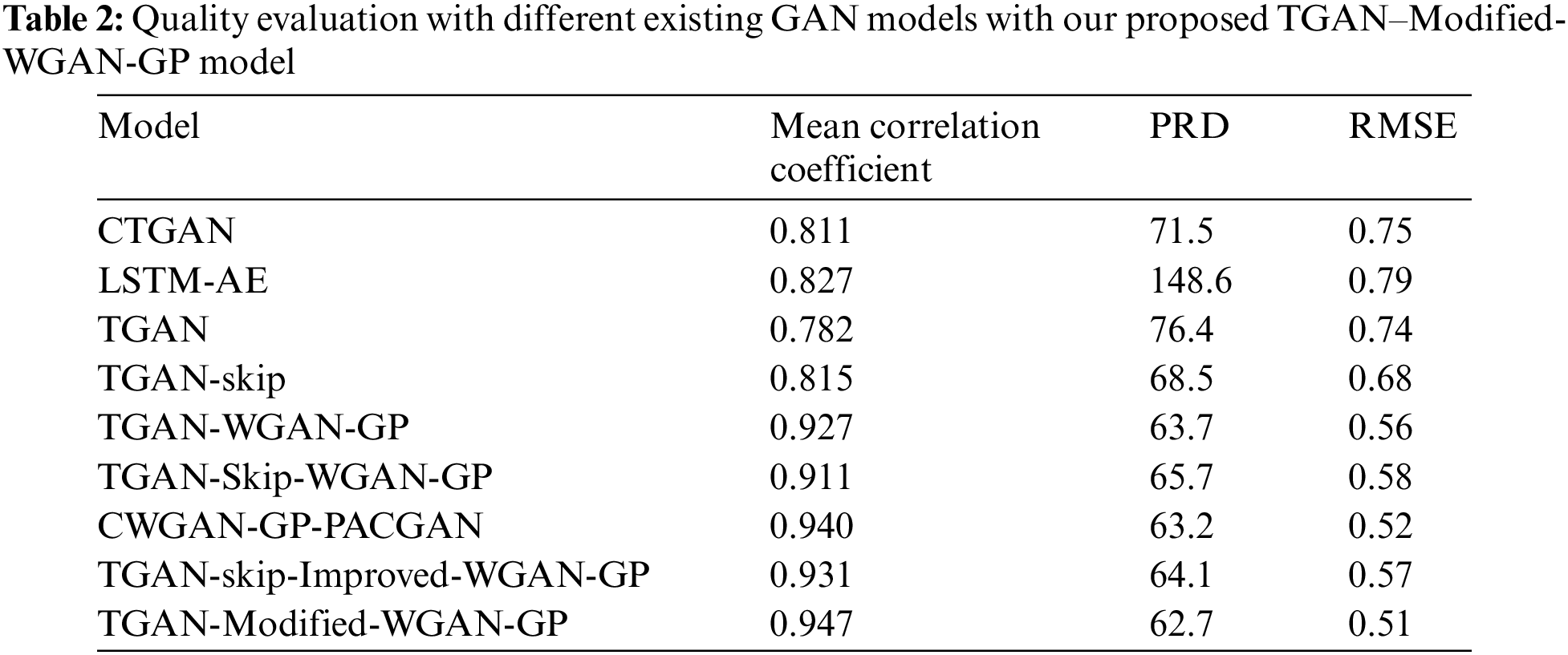
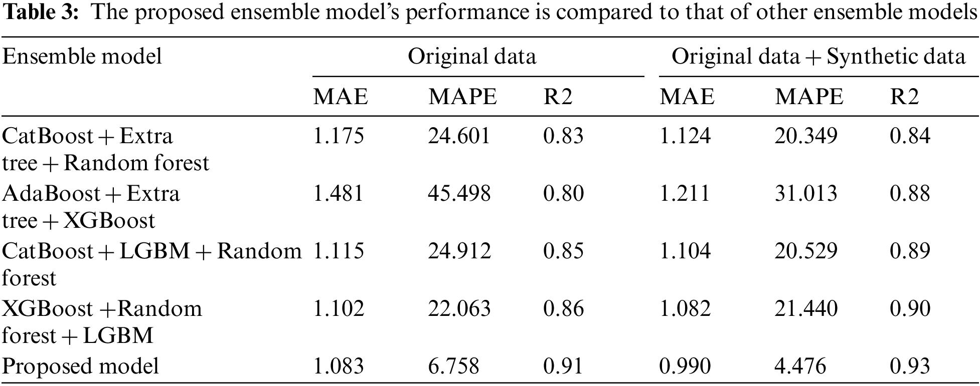
Table 3 presents the proposed model’s performance evaluation and a comparative analysis with counterpart conventional ensemble models. We have shown model results with original data, and combined data means original with synthetic data. The result depicts that the MAPE value decreased when original data was combined with synthetic data. In our experiment, 62% of the total data is synthetic data, and 38% of the total data is original data. Table 3 shows prediction model performance with original data and combined data that has been compared with other models. The performance of the suggested model is also compared to that of some previously developed ensemble models. The experimental results revealed that the proposed model outperforms all other standalone and ensemble models in terms of validation and testing. The performance analysis also demonstrates the model’s strength, which shows that it achieves a lower MAPE value and a higher R2 score than the baseline models. With original and synthetic data, our suggested ensemble prediction model got a MAPE of 4.476 and an R2 score of 0.93.

The suggested prediction model predicts the electric kickboard demand is based on time-series data from Jeju Island’s based mobility service provider. Fig. 5 shows the contrast between actual and predicted values. The red line indicates the actual value, and the blue line indicates the predicted value. This graph shows the impact of the proposed approach on the test data. We have used test data from the 1st of May 2021 to the 11th of June 2021. Here, the x-axis represents the date, and the y-axis shows the number of rent counts no rent number. As a result, the forecast is based on the training data. The proposed prediction model is trained with combined synthetic and original data. The larger dataset also enables the model to improve accuracy and reduce error rates on the test set. This indicates that our synthetic data is comparable to the training data we created and is more similar to the test data than the training data. Our proposed GAN model generates synthetic samples that reduce error and improve accuracy. It entails testing the trained model on a collection of held-out actual data after performing supervised training of a classifier on a synthetic dataset produced by the GAN. Since it illustrates that the synthetic data generated by the GAN can be used in practical applications, this evaluation metric is among the most well-liked ones.

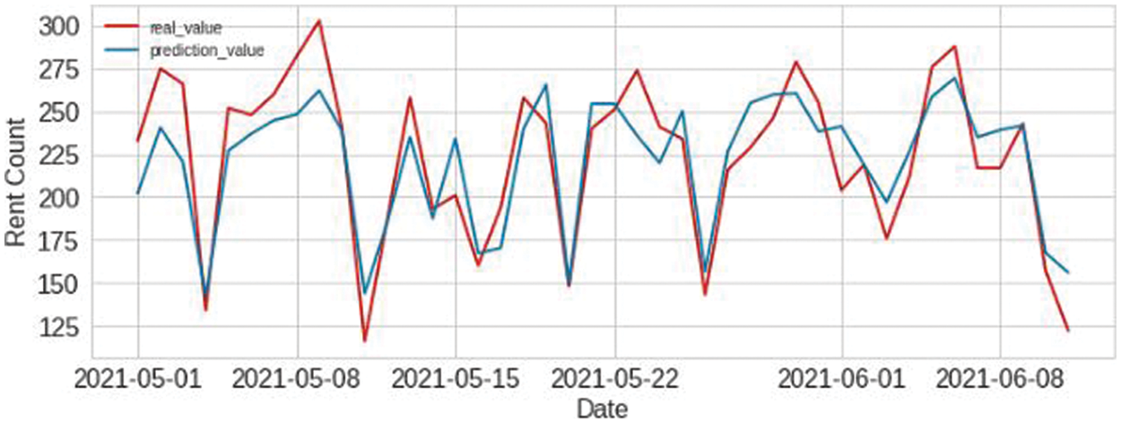
Figure 5: Prediction result of proposed method

The benefit of the work compared to alternative approaches is demonstrated in Table 4. For demand prediction, various ensemble strategies and a single model were developed. Here is a comparison of various approaches; we used the clustering methodology to segment regions. K-means clustering should be used using sectors 0, 1, 2, and 3. Then, we applied our suggested blended ensemble model to forecast demand. 20% of the total data were used for result testing, while the remaining 80% were trained. The prediction performance of other ensemble forecasting models is summarized in Table 3 to help you compare the performance of our proposed model to other models. As we can see, the blending ensemble learning model continues to produce the lowest prediction errors with original and synthetic data mixed with original data.

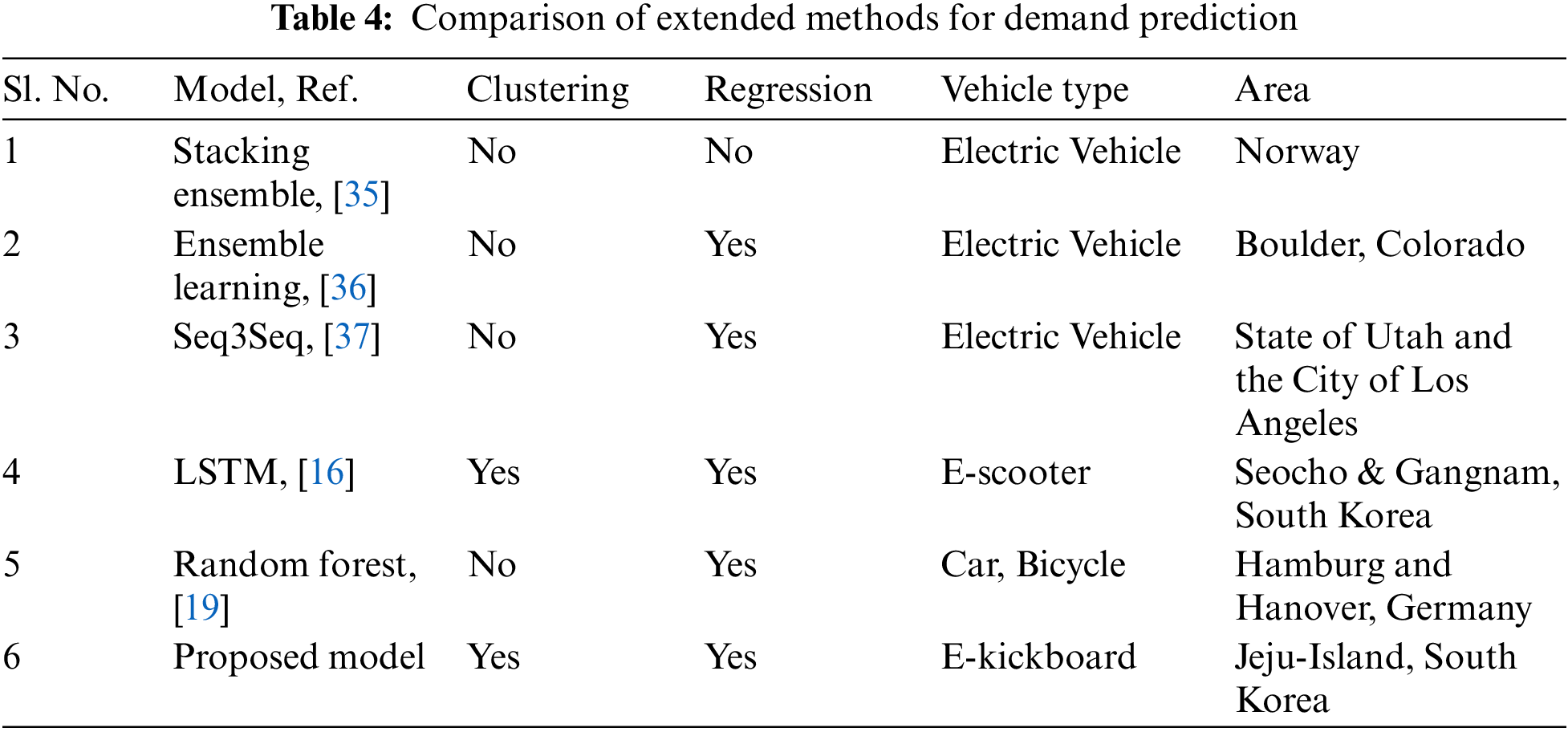
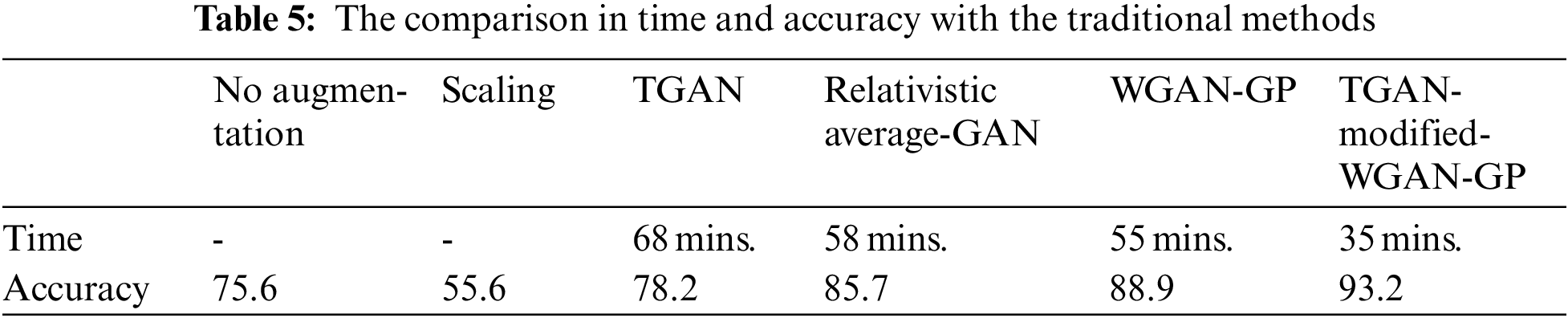
Fig. 5 displays the electric kickboard prediction outcomes using the suggested stacking technique-based blending ensemble model. The predicted values are provided in blue in this figure, whereas the actual values of the demand are displayed in red. The fact that the predicted values in the figure are too near to the actual values shows how well the suggested model predicts the demand for kickboards. The MAPE values in this graph roughly follow a line with a few peaks, which illustrates the stability of the proposed method for forecasting demand. The error rate in Table 3 demonstrates that the suggested model is not 100% reliable, and the error percentage is due to the divergence in prediction. In Table 5, we present the prediction accuracy along with the comparison of training time for different traditional methods. Synthetic data generated by individual GAN models and added with the original data for testing that depicts prediction accuracy is increased noticeably. The comparison of GPU training time of the traditional model is shown in Table 5. It is noticeable that the proposed TGAN-Modified-WGAN-GP takes less time than other conventional methods. We achieved better convergence after we modified the architecture with spectral normalization and RMSprop optimizer. We have depicted the time in minutes as mins.

4  Conclusion

The demand for electric mobility increases, especially in tourist areas and educational surrounded locality. ML can help accurately predict the electric mobility demand in the areas where companies struggle to meet the request at the proper location. In this article, we applied a regression-based blending ensemble technique that can help us to improve performance and increase accuracy based on three regressors models using a small amount of data for predicting demand of electric kickboard. We began our experiment by utilizing the data provided by a local electric kickboard service company. Mainly, tourists and locals peoples can hire electric kickboards from the company. Data smoothing maintained the general demand pattern while stabilizing the atypical pattern between the data. To anticipate demand, data with dissimilar features were segregated from data with similar features using clustering. For grouping and blending ensemble models for final prediction, we used the k means approach. The algorithms used in the blended ensemble model are XGBoost, extra tree, and random forest. We employed the additional tree model as a meta learner for the suggested model. As a result, the forecasting outcomes greatly improved, and the demand forecasting accuracy outcomes after Jeju Island’s regional split were also improved. We used our suggested strategy, and we were able to reach a MAPE of 4.4762. The findings of this study can be useful for electric mobility service providers who want to forecast demand precisely at a particular city location. The future perspective of the proposed approach will be used with other machine learning models in this research in order to take advantage of the ensemble models’ excellent performance.

Funding Statement: This work was supported by Korea Institute for Advancement of Technology (KIAT) grant funded by the Korea Government (MOTIE) (P0016977, The Establishment Project of Industry-University Fusion District).

Conflicts of Interest: The authors declare that they have no conflicts of interest to report regarding the present study.

References

 1.  G. Z. de Rubens, L. Noel, J. Kester and B. K. Sovacool, “The market case for electric mobility: Investigating electric vehicle business models for mass adoption,” Energy, vol. 194, pp. 116841, 2020. [Google Scholar]

 2.  K. Huang, G. H. de Almeida Correia and K. An, “Solving the station-based one-way carsharing network planning problem with relocations and non-linear demand,” Transportation Research Part C: Emerging Technologies, vol. 90, pp. 1–17, 2018. [Google Scholar]

 3.  C. A. Kennedy, N. Ibrahim and D. Hoornweg, “Low-carbon infrastructure strategies for cities,” Nature Climate Change, vol. 4, no. 5, pp. 343–346, 2014. [Google Scholar]

 4.  S. M. Raju, A. Sarker, A. Das, M. Islam, M. S. Al-Rakhami et al., “An approach for demand forecasting in steel industries using ensemble learning,” Complexity, vol. 2022, pp. 19, 2022. [Google Scholar]

 5.  M. H. Amini, O. Karabasoglu, M. D. Ilić, K. G. Boroojeni and S. S. Iyengar, “Arima-based demand forecasting method considering probabilistic model of electric vehicles’ parking lots,” in 2015 IEEE Power & Energy Society General Meeting, Denver, CO, USA, pp. 1–5, 2015. [Google Scholar]

 6.  H. Yu, X. Chen, Z. Li, G. Zhang, P. Liu et al., “Taxi-based mobility demand formulation and prediction using conditional generative adversarial network-driven learning approaches,” IEEE Transactions on Intelligent Transportation Systems, vol. 20, no. 10, pp. 3888–3899, 2019. [Google Scholar]

 7.  C. Zhang, F. Zhu, Y. Lv, P. Ye and F. Y. Wang, “MLRNN: Taxi demand prediction based on multi-level deep learning and regional heterogeneity analysis,” IEEE Transactions on Intelligent Transportation Systems, vol. 23, no. 7, pp. 8412–8422, 2021. [Google Scholar]

 8.  D. Cao, K. Zeng, J. Wang, P. K. Sharma, X. Ma et al., “BERT-Based deep spatial-temporal network for taxi demand prediction,” IEEE Transactions on Intelligent Transportation Systems, vol. 23, no. 7, pp. 9442–9454, 2021. [Google Scholar]

 9.  G. Van Kriekinge, C. De Cauwer, N. Sapountzoglou, T. Coosemans and M. Messagie, “Day-ahead forecast of electric vehicle charging demand with deep neural networks,” World Electric Vehicle Journal, vol. 12, no. 4, pp. 178, 2021. [Google Scholar]

10. R. Wang, S. Lu and W. Feng, “A novel improved model for building energy consumption prediction based on model integration,” Applied Energy, vol. 262, pp. 114561, 2020. [Google Scholar]

11. M. Rezagholiradeh and M. A. Haidar, “Reg-gan: Semi-supervised learning based on generative adversarial networks for regression,” in 2018 IEEE Int. Conf. on Acoustics, Speech and Signal Processing, Calgary, AB, Canada, pp. 2806–2810, 2018. [Google Scholar]

12. C. Tian, C. Li, G. Zhang and Y. Lv, “Data driven parallel prediction of building energy consumption using generative adversarial nets,” Energy and Buildings, vol. 186, pp. 230–243, 2019. [Google Scholar]

13. K. Zhang, G. Zhong, J. Dong, S. Wang and Wang Y., “Stock market prediction based on generative adversarial network,” Procedia Computer Science, vol. 147, pp. 400–406, 2019. [Google Scholar]

14. D. Hazra, W. Shafqat and Y. Byun, “Generating synthetic data to reduce prediction error of energy consumption,” Computers, Materials & Continua, vol. 70, no. 2, pp. 3151–3167, 2022. [Google Scholar]

15. D. Sami Khafaga, A. Ali Alhussan, E. M. El-kenawy, A. Ibrahim, S. H. Abd Elkhalik et al., “Improved prediction of metamaterial antenna bandwidth using adaptive optimization of lstm,” Computers, Materials & Continua, vol. 73, no. 1, pp. 865–881, 2022. [Google Scholar]

16. S. Kim, S. Choo, G. Lee and S. Kim, “Predicting demand for shared e-scooter using community structure and deep learning method,” Sustainability, vol. 14, no. 5, pp. 2564, 2022. [Google Scholar]

17. S. Kim, U. Lee, I. Lee and N. Kang, “Idle vehicle relocation strategy through deep learning for shared autonomous electric vehicle system optimization,” Journal of Cleaner Production, vol. 333, pp. 130055, 2022. [Google Scholar]

18. Z. Yi, X. C. Liu and R. Wei, “Electric vehicle demand estimation and charging station allocation using urban informatics,” Transportation Research Part D: Transport and Environment, vol. 106, pp. 103264, 2022. [Google Scholar]

19. F. Zwick and K. W. Axhausen, “Ride-pooling demand prediction: A spatiotemporal assessment in Germany,” Journal of Transport Geography, vol. 100, pp. 103307, 2022. [Google Scholar]

20. I. Goodfellow, J. Pouget-Abadie, M. Mirza, B. Xu, D. Warde-Farley et al., “Generative adversarial nets,” Advances in Neural Information Processing Systems, vol. 27, pp. 2672–2680, 2014. [Google Scholar]

21. L. Xu and K. Veeramachaneni, “Synthesizing tabular data using generative adversarial networks,” Computing Research Repository (CoRR), vol. abs, pp. 1181.11264, 2018. [Google Scholar]

22. I. Gulrajani, F. Ahmed, M. Arjovsky, V. Dumoulin and A. C. Courville, “Improved training of wasserstein gans,” Advances in Neural Information Processing Systems, vol. 30, pp. 5767–5777, 2017. [Google Scholar]

23. M. Arjovsky, S. Chintala and L. Bottou, “Wasserstein generative adversarial networks,” in Proc. of the 34th Int. Conf. on Machine Learning, Sydney, NSW, Australia, vol. 70, pp. 214–223, 2017. [Google Scholar]

24. B. K. Iwana and S. Uchida, “Time series data augmentation for neural networks by time warping with a discriminative teacher,” in 2020 25th Int. Conf. on Pattern Recognition, Milan, Italy, pp. 3558–3565, 2021. [Google Scholar]

25. T. Miyato, T. Kataoka, M. Koyama and Y. Yoshida, “Spectral normalization for generative adversarial networks,” in Int. Conf. on Learning Representations, Vancouver Convention Center, Vancouver, BC, Canada, pp. 1802.05957, 2018. [Google Scholar]

26. J. A. Hartigan and M. A. Wong, “Algorithm AS 136: A k-means clustering algorithm,” Journal of the Royal Statistical Society. Series C (Applied Statistics), vol. 28, no. 1, pp. 100–108, 1979. [Google Scholar]

27. A. M. Fahim, A. M. Salem, F. A. Torkey and M. A. Ramadan, “An efficient enhanced k-means clustering algorithm,” Journal of Zhejiang University-Science A, vol. 7, no. 10, pp. 1626–1633, 2006. [Google Scholar]

28. P. Geurts, D. Ernst and L. Wehenkel, “Extremely randomized trees,” Machine Learning, vol. 63, no. 1, pp. 3–42, 2006. [Google Scholar]

29. X. Wang, T. Liu, X. Zheng, H. Peng, J. Xin et al., “Short-term prediction of groundwater level using improved random forest regression with a combination of random features,” Applied Water Science, vol. 8, no. 5, pp. 1–12, 2018. [Google Scholar]

30. L. Torlay, M. Perrone-Bertolotti, E. Thomas and M. Baciu, “Machine learning–XGBoost analysis of language networks to classify patients with epilepsy,” Brain Informatics, vol. 4, no. 3, pp. 159–169, 2017. [Google Scholar]

31. F. Ma and X. Yan, “Research on the energy consumption estimation method of pure electric vehicle based on XGBoost,” in 2019 3rd Int. Conf. on Electronic Information Technology and Computer Engineering, Xiamen, China, pp. 1021–1026, 2019. [Google Scholar]

32. Y. Zhan, Y. Luo, X. Deng, M. L. Grieneisen, M. Zhang et al., “Spatiotemporal prediction of daily ambient ozone levels across China using random forest for human exposure assessment,” Environmental Pollution, vol. 233, pp. 464–473, 2018. [Google Scholar]

33. M. W. Ahmad, J. Reynolds and Y. Rezgui, “Predictive modelling for solar thermal energy systems: A comparison of support vector regression, random forest, extra trees and regression trees,” Journal of Cleaner Production, vol. 203, pp. 810–821, 2018. [Google Scholar]

34. R. W. Emerson, “Causation and Pearson’s correlation coefficient,” Journal of Visual Impairment & Blindness, vol. 109, no. 3, pp. 242–244, 2015. [Google Scholar]

35. S. Ai, A. Chakravorty and C. Rong, “Household EV charging demand prediction using machine and ensemble learning,” in 2018 IEEE Int. Conf. on Energy Internet, Beijing, China, pp. 163–168, 2018. [Google Scholar]

36. X. Huang, D. Wu and B. Boulet, “Ensemble learning for charging load forecasting of electric vehicle charging stations,” in 2020 IEEE Electric Power and Energy Conf., Edmonton, AB, Canada, pp. 1–5, 2020. [Google Scholar]

37. Z. Yi, X. C. Liu, R. Wei, X. Chen and J. Dai, “Electric vehicle charging demand forecasting using deep learning model,” Journal of Intelligent Transportation Systems, vol. 2021, pp. 1–14, 2021. [Google Scholar]