Modeling of Computer Virus Propagation with Fuzzy Parameters

1  Introduction

A type of malicious program that, once executed, duplicates itself by modifying several sensitive products and inserting them into its specific code is called a computer virus. Boot sector virus, multipart virus, macro virus, program virus, polymorphic virus, etc., are some common types of computer viruses. The thought processes behind creating viruses are monetary gain, sending public messages, making someone happy, and showing that some flaws are there in the framework. A common virus, therefore, fulfills two functions. Firstly, it duplicates itself in uninfected projects, files, or programs. Then, it carries out other vengeful instructions given by the virus designer. Virus scientists use strategies such as padding, pressing, and encrypting spaces to avoid detection. At the same time, antivirus projects use other static and dynamic approaches to identify the virus. Some widespread computer viruses are program downloads, pirated or decrypted software, email connections, the web, obscure Compact Disk (CD) boot information, unpatched applications, and Bluetooth. Symptoms, for example, the partition disappears completely, there is no reaction from the programs that are used to run it because some files are missing, the windows do not start, error messages appear with the records missing without the process uninstall, a program disappears from the Personal Computer (PC), new symbols appear by themselves in the work area, the PC does not allow the reintroduction of antivirus programming, an opaque explanation means that antivirus programming is blocked and cannot be restarted, a strange connection is made via an e-mail Message established, the PC cannot update the antivirus programming, then, the email account sends infected messages to our contacts, we cannot open documents and reports, problems in reopening destroyed data whose design has been changed, it is difficult to draw the best of an application, music or unusual noises on the speakers and activities crashes and the PC shows annoying messages when it keeps booting apart from undetected errors your PC is taking a long time to start making it easier to run, etc. cannot be seen on an infected PC [1]. The “Creeper System” was the first computer virus discovered in 1971. BBN Innovations caused an infection in the United States. In 1982, a virus known as “Elk Cloner” was found. In 1986, the first MS-DOS “Brain” computer virus was discovered, which had the utility to prevent the PC from booting and overwriting the bootable area on the floppy disk. “The Morris” appeared and infected countless populations of personal computers in 1988. The virus, discovered in Australia in 1991 without precedent, has been named “Michelangelo”. Two years after Windows 3.0, in April 1992, we learned that a virus was attacking MS Windows. “Melissa” was released in 1999. In 2000, the “I love you” infection returned and emailed itself to all contacts.

A latently infected computer that cannot infect other computers simultaneously is called an exposed computer. However, there is a possibility of infection. Yang et al. proposed the Susceptible, Latent and Breaking out (SLB) computer model and the Susceptible, Latent and Breaking out, Susceptible (SLBS) computer model [2]. The computer was considered infectious during the latency period. Mishra et al. studied a Susceptible–Exposed–Infectious–Quarantined–Recovered (SEIQR) computer virus model [3]. Many other authors have also investigated the spread of computer viruses in the past by creating mathematical models [4–11]. SLBS computer model was developed by Yang et al. to study virus propagation [2]. Ahmed et al. proposed a Spatio-temporal computer virus model [12]. Ali et al. studied virus propagation through padé approximation [13]. Ebenezer et al. studied a fractional model of a computer virus by developing interaction between computers and removable devices [14]. Lanz et al. presented a virus model with the strategy of quarantine [15]. Xu et al. proposed a new model with a limited ability of the antivirus [16]. Parsaei et al. developed a new mathematical model of computer viruses [17]. Deng et al. presented a Susceptible, Infected, Recovered, Dead (SIRD) computer virus model and examined the transmission mechanisms of the virus [18]. Tuwairqi et al. has proposed two computer virus-propagation isolation strategies [19].

The fuzzy theory was introduced by Zadeh in 1965 [20]. Barros et al. [21] and Mondal et al. [22] examined epidemic models with fuzzy transmission coefficients. A fuzzy Susceptible–Infected–Recovered (SIR) model was proposed by Abdy et al. [23]. Ortega et al. [24] used fuzzy logic to predict the epidemiological problems associated with infectious diseases. The transmission of worms in computer networks was studied by Mishra et al. through a fuzzy Susceptible–Infectious––Recovered–Susceptible (SIRS) and a fuzzy Susceptible–Exposed–Infectious–Quarantined–Recovered–Susceptible (SEIQRS) model [25,26]. The low, medium, and high cases of outbreak control of worms on the computer network have been analyzed to understand better the worm attack, which can also control them. NSFD theory introduced by Mickens [27] is extensively used in the mathematical and numerical modeling of diseases. Allehiany et al. studied the COVID-19 dynamics using NSFD in fuzzy senses [28]. Dayan et al. developed an NSFD scheme to observe the spread of rumors and coronavirus dynamics [29,30]. Fuzzy theory is being applied in many other fields very frequently. Khokhar et al. presented a fuzzy logic controller to improve the performance and accuracy of the system, which also improved the efficiency of the cost and energy [31,32], for example.

As with many other research questions on the spread of the virus, a reliable assessment of transmission dynamics is an essential part of the investigation. Collecting numerical data as a fixed value is a challenging task in many situations in daily life. Different degrees of infectivity and recovery from the infection among the considered PCs may raise uncertainties. Various sizes, models, spare parts, the surrounding environments of these PCs, and many other factors, like the resistance capacity of the individual PC against the virus, are some of the reasons for these uncertainties. Each personal PC has a different degree of infectivity and resistance against infection. In this scenario, the fuzzy model has richer dynamics than its classical counterpart in epidemiology. Keeping this in mind, a computer virus model with fuzzy parameters is developed in this study. The current work is an extension of the computer virus propagation model studied by Arif et al. by introducing fuzzy parameters, which makes it possible to explain the spread of viruses in computers in more detail. The novelty of the developed technique is the construction, execution, and mathematical analysis of the explicit first-order scheme in fuzzy environments with NSFD settings, particularly with fuzzy parameters. To our knowledge, the studied model has not been analyzed before in a fuzzy sense in the literature, and this is the first study of this model in this regard. The rest of this study is designed as some definitions and formulations of the fuzzy model are presented in Section 2. Numerical modeling is carried out in Section 3. Section 4 contains the resulting numerical solution and simulation results. Conclusions and future directions are presented in Section 5.

2  Computer Virus Propagation Model with Fuzzy Parameters

2.1 Definition 1 [33]

A subset S of the set U denoted by μS(u):U→[0,1], where μS(u) shows the membership degree of u in S, is called a fuzzy subset.

2.2 Definition 2 [33]

The number A=(ω1,ω2,ω3) is a triangular fuzzy number (TFN) if it is given by

μA(t)={0,t<ω1t−ω1ω2−ω1,ω1≤t≤ω2ω3−tω3−ω2,ω2≤t≤ω30,t>ω3.

where ω1≤ω2≤ω3.

2.3 Definition 3 [34]

The expected value of a TFN A is given by

E[A]=a+2b+c4.

2.4 Definition 4

The fuzzy basic reproductive number R0f is defined as R0f=E[R0(v)].

We considered the computer virus propagation model that has been talked about by Arif et al.

S′=δ−βS(L+B)+γB−δS,(1)

L′=βS(L+B)−αL−δL,(2)

B′=αL−γB−δB.(3)

The corresponding SLB model with fuzzy parameters is

S′=δ−β(a)S(L+B)+γ(a)B−δS,(4)

L′=β(a)S(L+B)−αL−δL,(5)

B′=αL−γ(a)B−δB.(6)

The parameters S denotes susceptible, L means latent, and B denotes breaking out computers. α is the number of break-out latent PCs, β is the speed at which an infected PC damages a virus-free PC, γ is the rate of recovery of breaking-out PCs, and the speed with which systems connect to the Internet and internal systems connected are separated from the global network is indicated by δ. The presence or absence of the virus in computer virus propagation models is essential to distinguish breaking-out PCs from susceptible PCs. We consider the model’s heterogeneity by considering the infection in each PC as a function of the virus load. We assume that all infected PCs do not have the same contribution to the virus transmission process. Each PC has a different degree of infectivity, depending on the virus’s quantity. The parameters β(a) and γ(a) can be displayed as a function of the computer virus load a. The greatest chance of virus transmission is when the virus load is at its highest. The graphical representation of the parameter β(a) is defined as

β(a)={0,a<ama−ama0−am,am≤a≤a01,a0<a.(7)

The recovery rate γ=γ(a) given below is also assumed to be a fuzzy number.

γ(a)={(γ0−1)aa0+1,0≤a≤a0γ0,a0≤a.(8)

γ0>0 is the minimum recovery rate. The membership function of β(a) and γ(a) are shown in Fig. 1.

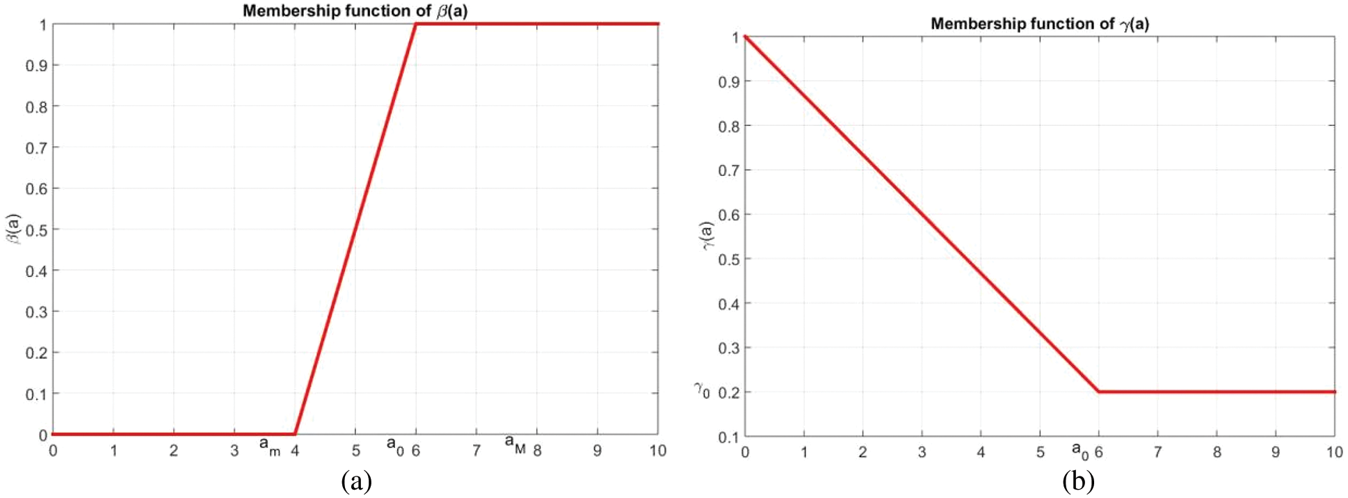
Figure 1: The membership function of (a) β(a) and (b) γ(a)

2.5 The Fuzzy Basic Reproductive Number Rcf

Rc is calculated using next-generation matrix theory and given by Rc=β(a)α+γ(a).

Rc being a function of virus load is examined for various amounts of the virus as

Case 1: If a<amin, β(a)=0, then Rc(a)=0.

Case 2: If amin<a≤aM, β(a)=a−aminaM−amin and Rc(a)=a−amin(α+γ(a))(aM−amin).

Case 3: If aM<a<amax, β(a)=1 and Rc(a)=1α+γ(a).

Rc(a) can be expressed as a TFN as:

Rc(a)=(0,β(a)α+γ(a),1α+γ(a)).

Now we find Rcf as follows:

Rcf=E[Rc(a)]=2β(a)+14(α+γ(a)).

2.6 Fuzzy Equilibrium Analysis

Case 1: If a<amin and β(a)=0, we get S=1, L=0 and B=0. Therefore, we obtain

E0=(S0,L0,B0)=(1,0,0),

which is the virus-free equilibrium point. It is the situation when no virus exists in the computer.

Case 2: If amin<a≤aM, then β(a)=a−aminaM−amin, and we get E∗=(S∗,L∗,B∗), where,

S∗=δ(α+δ)2+δγ(a)(2δ+α+γ(a))+α(δ−α)+αγ(a)β(a)(δ+γ(a))(δ+γ(a)+2α),

L∗=(α+δ+γ(a))(β(a)−δ)−αγ(a)β(a)(δ+γ(a)+2α)

andB∗=α[αβ(a)−δ(α+δ)+γ(a)(β(a)−1)]β(a)(δ+γ(a))(δ+γ(a)+2α).

Case 3: If aM<a<amax, then β(a)=1 and we obtain E∗∗=(S∗∗,L∗,B∗∗), where,

S∗∗=δ(α+δ)2+δγ(a)(2δ+α+γ(a))+α(δ−α)+αγ(a)(δ+γ(a))(δ+γ(a)+2α),

L∗∗=(α+δ+γ(a))(1−δ)−αγ(a)(δ+γ(a)+2α)

andB∗∗=α[α−δ(α+δ)](δ+γ(a))(δ+γ(a)+2α).

3  Numerical Modeling

3.1 Forward Euler Scheme

Forward Euler scheme for the system (4–6) can be written as

sn+1=sn+h[δ−β(a)sn(ln+bn)+γ(a)bn−δsn],(9)

ln+1=ln+h[β(a)sn(ln+bn)−αln−δln],(10)

bn+1=bn+h[ln−γ(a)bn−δbn].(11)

Here we focus on the model in a fuzzy environment of a specific group of PCs with a triangular membership function. We examine it for different amounts of viruses.

Case 1: If a<amin, then β(a)=0, and the above system becomes

sn+1=sn+h[δ+γ(a)bn−δsn],

ln+1=ln−h[αln+δln],

bn+1=bn+h[ln−γ(a)bn−δbn].

Case 2: If amin<a≤aM, then β(a)=a−aminaM−amin, and the above system becomes

sn+1=sn+h[δ−β(a)sn(ln+bn)+γ(a)bn−δsn],

ln+1=ln+h[β(a)sn(ln+bn)−αln−δln],

bn+1=bn+h[ln−γ(a)bn−δbn].

Case 3: If aM<a<amax, then β(a)=1, and the above system becomes

sn+1=sn+h[δ−sn(ln+bn)+γ(a)bn−δsn],

ln+1=ln+h[sn(ln+bn)−αln−δln],

bn+1=bn+h[ln−γ(a)bn−δbn].

3.2 Nonstandard Finite Difference (NSFD) Scheme

NSFD scheme for the system (4–6) can be written as

sn+1=sn+hδ+hγ(a)bn1+hβ(a)(ln+bn)+hδ,

ln+1=ln+hβ(a)sn+1(ln+bn)1+h(α+δ),

bn+1=bn+hαln+11+h(γ(a)+δ).

Again, we examine the above scheme for different amounts of viruses as we focus on the model in a fuzzy environment of a specific group of PCs with a triangular membership function.

Case 1: If a<amin, then β(a)=0, and the above system becomes

sn+1=sn+hδ+hγ(a)bn1+hδ,

ln+1=ln1+h(α+δ),

bn+1=bn+hαln+11+h(γ(a)+δ).

Case 2: If amin<a≤aM then β(a)=a−aminaM−amin and the above system becomes

sn+1=sn+hδ+hγ(a)bn1+hβ(a)(ln+bn)+hδ,

ln+1=ln+hβ(a)sn+1(ln+bn)1+h(α+δ),

bn+1=bn+hαln+11+h(γ(a)+δ).

Case 3: If aM<a<amax, then β(a)=1, and the above system becomes

sn+1=sn+hδ+hγ(a)bn1+h(ln+bn)+hδ,

ln+1=ln+hsn+1(ln+bn)1+h(α+δ),

bn+1=bn+hαln+11+h(γ(a)+δ).

3.3 Stability of the NSFD Scheme

Let

M1=sn+hδ+hγ(a)bn1+hβ(ln+bn)+hδ,

M2=ln+hβsn+1(ln+bn)1+h(α+δ),

M3=bn+hαln+11+h(γ(a)+δ).

Jacobian of the above equations can be written as

J=[11+hβ(a)(l+b)+hδ−hβ(a)(s+hδ+hγ(a)b)[1+hβ(a)(l+b)+hδ]2h(γ(a)+hδlβ(a)−hδ)[1+hβ(a)(l+b)+hδ]2hβ(a)(l+b)1+h(α+δ)1+hβ(a)s1+h(α+δ)hβ(a)s1+h(α+δ)0hα1+h(γ(a)+δ)11+h(γ(a)+δ)]

The above Jacobian at the VFE becomes,

J1=[11+hδ0hγ(a)−h2δ(1+hδ)2011+h(α+δ)00hα1+h(γ(a)+δ)11+h(γ(a)+δ)]

The above numerical scheme will be unconditionally convergent if and only if the absolute eigenvalues of the above Jacobian matrix are less than unity, i.e., |λi|<1,i=1,2,3.We obtain the Eigen values λ1=11+hδ<1, λ2=11+h(γ(a)+δ)<1 and λ3=11+h(α+δ)<1 from the Jacobian matrix J1. All eigenvalues are less than unity which is the desired result.

4  Numerical Simulations

Numerical simulations for the above schemes are presented below. The behavior of the fuzzy SLB model can be examined in these graphs.

In Fig. 2, the portions of susceptible computers are represented using Euler and NSFD schemes at different step sizes at the VFE point. The results indicate that the Euler method converges for a small value of the time step size h=1. It oscillates in a nonphysical manner as we increase the value of the step size to h=1.8. The NSFD method remains convergent and reflects a positive behavior at all step size values.

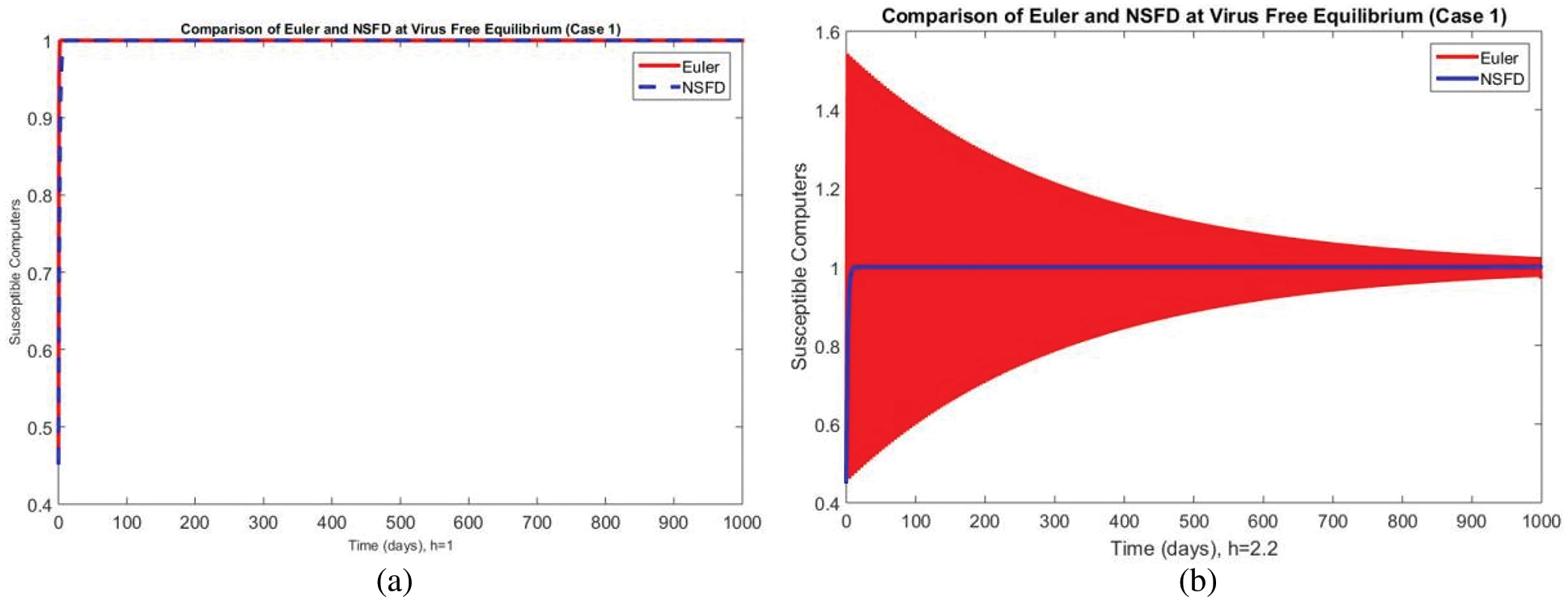
Figure 2: Portion of susceptible computers using Euler and NSFD schemes at (a) h=1, (b) h=2.2

The portions of latent computers are shown in Fig. 3 using Euler and NSFD schemes at different step sizes at the VFE point. It can be seen in the graphs that the Euler scheme converges initially for a small value of the step size and creates negative values by increasing the value of h. The method also starts nonphysical oscillations at the increased step size. On the other hand side, the NSFD method converges to the steady-state despite changing the step sizes.

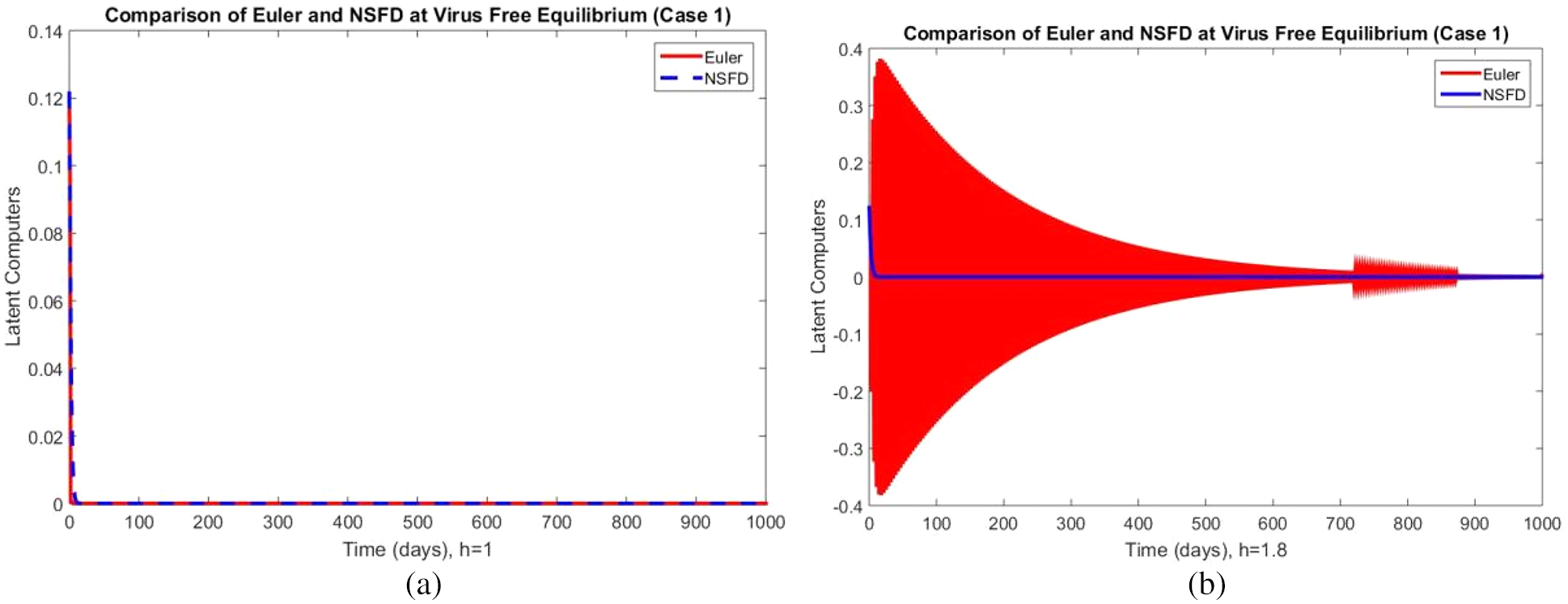
Figure 3: Portion of latent computers using Euler and NSFD schemes at (a) h=1, (b) h=1.8

Fig. 4 shows the solution results of the breaking out computers at two different values of the step size h. The Euler method behaves well at a smaller value of h, but oscillations get started with a slight increase in the value of h, and the technique produces negative results as well. The NSFD approach, on the other hand, side is independent of the importance of h and gives the same convergent results in all cases.

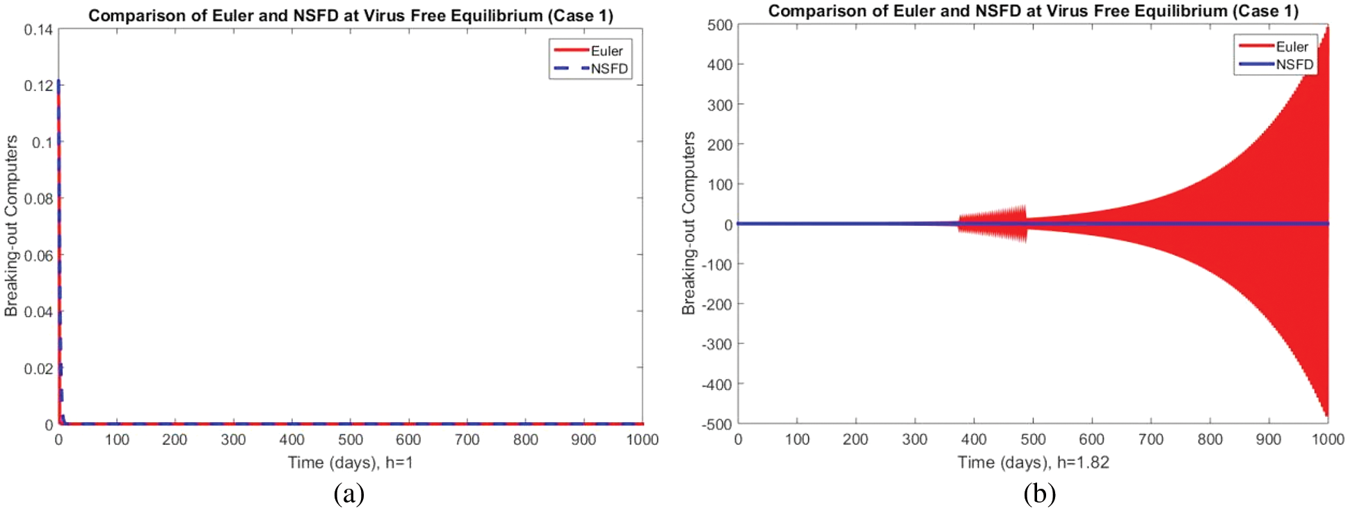
Figure 4: Portion of computer breaking using Euler and NSFD schemes at (a) h=1, (b) h=1.82

The simulation results of compartment S for case 2 are depicted in Fig. 5. The behavior of Euler’s scheme at the start looks well for a smaller value. Still, it makes vast oscillations as we increase the step size and fails to converge smoothly. The NSFD still shows its converging behavior.

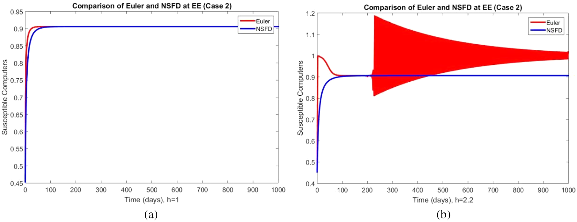
Figure 5: Portion of susceptible computers using Euler and NSFD schemes at (a) h=1, (b) h=2.2

In Fig. 6, the numerical experiments of compartment L are represented at the first endemic equilibrium point. Again, we observe the positivity and convergence solutions of the NSFD method at both step sizes. Euler’s method remains positive and convergent for the smaller value and fails to produce positive and convergent solutions at increased step size.

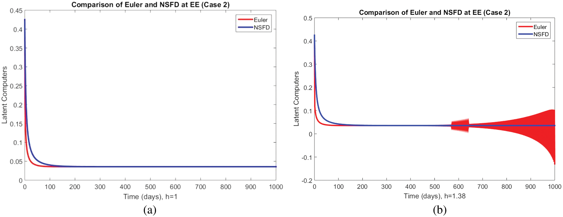
Figure 6: Portion of latent computers using Euler and NSFD schemes at (a) h=1, (b) h=1.38

Positive and convergent solutions of Euler’s scheme at a small value representing compartment B for case 2 can be seen in Fig. 7. The change in step size makes Euler’s method fail to converge.

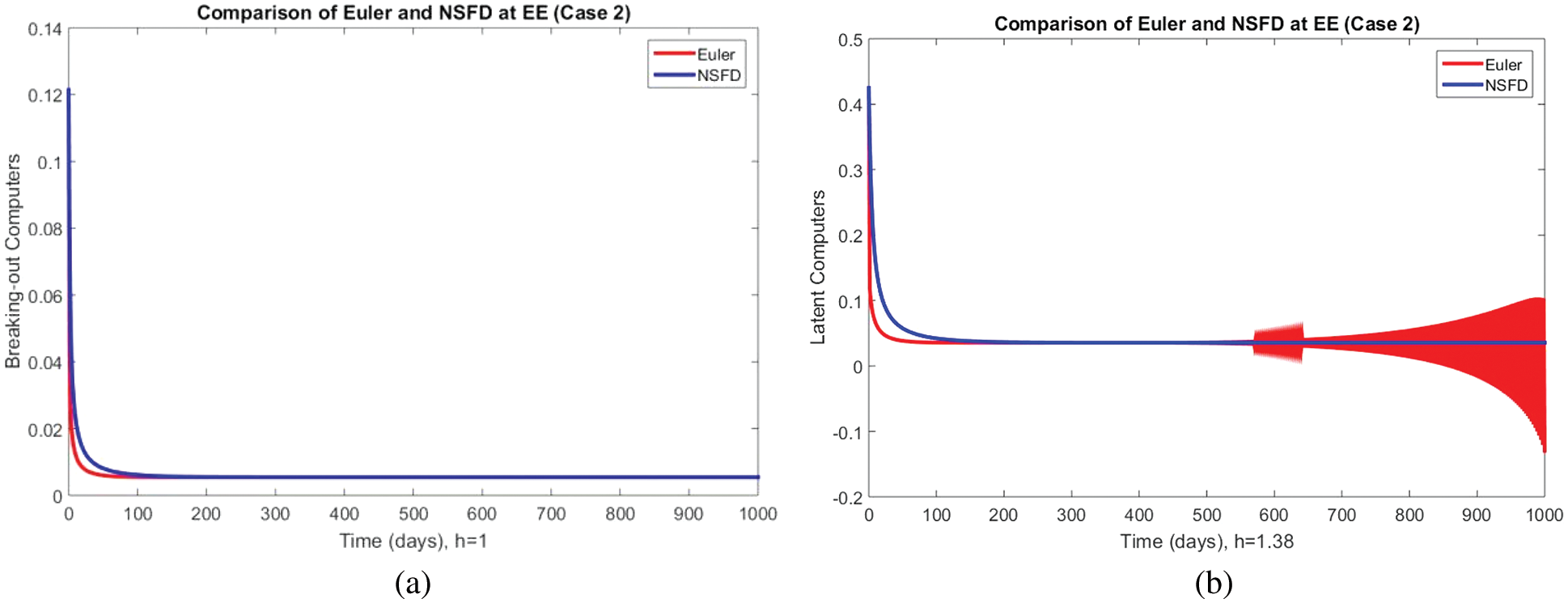
Figure 7: Portion of computer breaking using Euler and NSFD schemes at (a) h=0.1, (b) h=10

In Figs. 8–10, the portions of all model compartments are represented at the second endemic equilibrium point. The positivity and convergence solutions of the developed method are reflected again. The non-convergence behavior of Euler’s approach at a slightly higher value remains the same. One of the most exciting features of the above graphs is the consistency of the NSFD method across all step sizes, as many other classical methods such as Euler Maruyama, Euler’s Stochastic, and RK-4 do not preserve it at large step sizes, as discussed in [35–49]. Standard finite difference schemes and stochastic techniques violate dynamical properties and produce negative and unbounded solutions that have no physical meaning, as discussed by Arif et al. Finite difference techniques with fuzziness exhibit similar behavior.

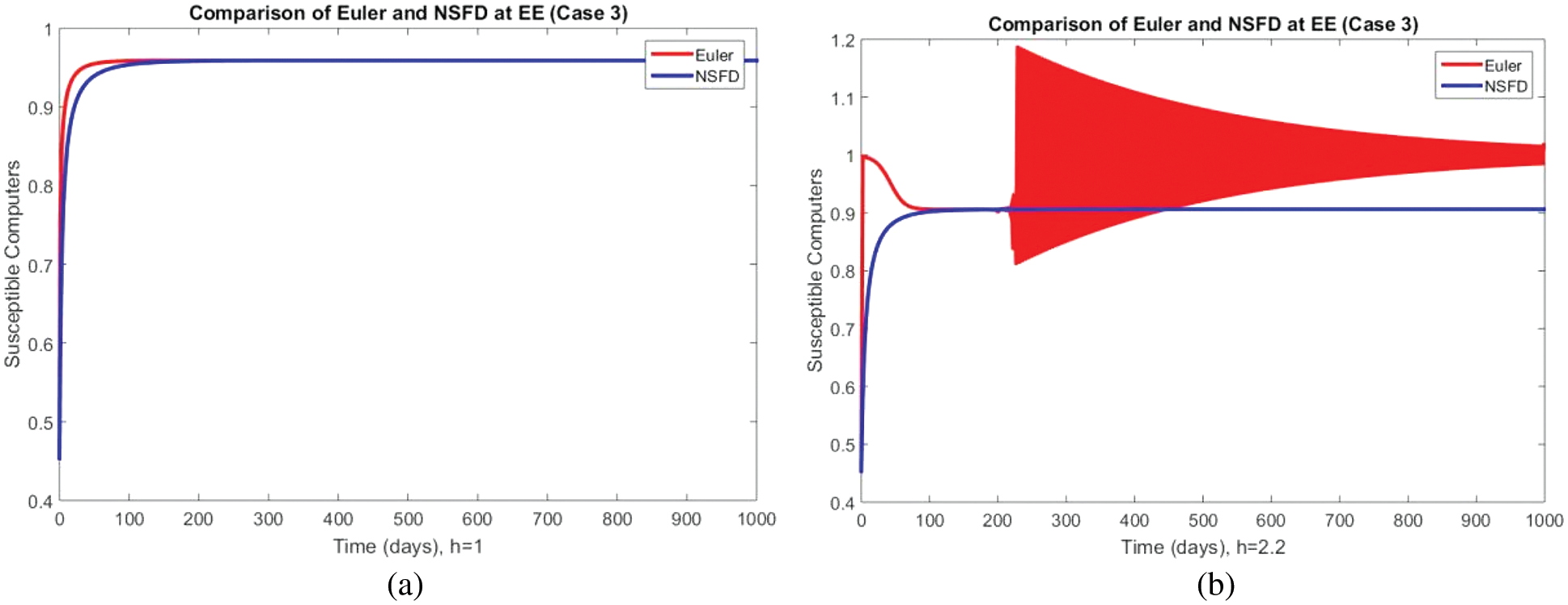
Figure 8: Portion of susceptible computers using Euler and NSFD schemes at (a) h=1, (b) h=2.2

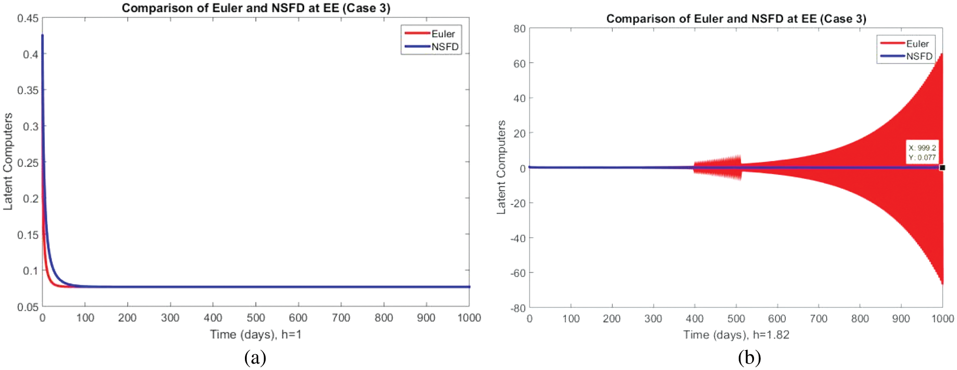
Figure 9: Portion of latent computers using Euler and NSFD schemes at (a) h=1, (b) h=1.82

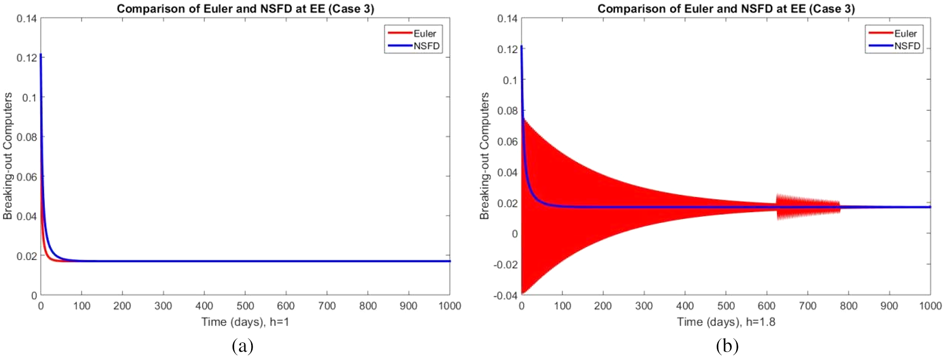
Figure 10: Portion of computer breaking using Euler and NSFD schemes at (a) h=1, (b) h=1.8

On the other hand, the NSFD with fuzziness preserves the essential features of the epidemic model. Maintaining the dynamic constraints results in a model exhibiting good dynamic behavior even over large increments. This also gives a great implementation and computational advantage.

5  Conclusion

The numerical analysis of the computer virus propagation model with fuzzy parameters by introducing forward Euler and NSFD techniques is presented in this study with the assumption that the virus transmission and the recovery of the infected computers are not the same for all PC’s under consideration. These are treated as fuzzy numbers depending on the amount of the virus on the single individual PC. In classical models, each parameter is assigned a fixed value independent of the virus load. In this context, the model with fuzziness is more valuable and reliable. A comparison of both methods is presented, which shows the dynamical consistency of our proposed NSFD numerical scheme for the studied model. Euler’s approach could not produce convergent solutions at slightly significant time steps. The newly proposed technique is found to be positivity preserving and convergent through simulation results. The NSFD technique is, therefore, easy to implement, which shows stable behavior numerically and demonstrates a good agreement with analytic results possessed by the continuous model. Thus, the NSFD technique is easy to implement, exhibits normal numerical behavior, and shows a good deal with the analytical results of the continuous model. The current study is unique because it is the first attempt to analyze a computer virus model using Euler’s method and the NSFD scheme with fuzziness. The results obtained are new for the model. The proposed NSFD method preserves stability, equilibrium convergence, and positivity at all step sizes.

In comparison, most other standard procedures do not preserve these essential characteristics of the epidemic system. The biggest strength of the proposed approach is that it performs well for all parameter options and initial and step size values, which can also be seen in the graphs discussed in the article. In this work, we analyze the epidemic model of propagation of computer viruses for a general class of parameters taken from the scientific literature. We plan to apply these results to real-time data. The current work mainly focuses on including fuzzy triangular numbers as membership functions. The trapezoidal, pentagonal, and other fuzzy numbers can also be used as membership functions which may also be our future directions. Stochastic, delayed, and fractional dynamics with the fuzziness of the studied model can also be considered as a future direction.

Acknowledgement: The authors are thankful to the Govt. of Pakistan for providing the facility to conduct the research. All Authors are grateful for the suggestions of anonymous referees to improve the quality of the manuscript.

Funding Statement: The authors received no specific funding for this study.

Conflicts of Interest: The authors declare they have no conflicts of interest to report regarding the present study.

References

1. M. S. Arif, A. Raza, M. Rafiq, M. Bibi, J. N. Abbasi et al., “Numerical simulations for stochastic computer virus propagation model,” Computers, Materials and Continua, vol. 62, no. 1, pp. 61–77, 2020. [Google Scholar]
2. L. X. Yang, X. Yang, L. Wen and J. Liu, “A novel computer virus propagation model and its dynamics,” International Journal of Computer Mathematics, vol. 89, no. 17, pp. 2307–2314, 2012. [Google Scholar]
3. B. K. Mishra and N. Jha, “SEIQRS model for the transmission of malicious objects in computer network,” Applied Mathematical Modelling, vol. 34, no. 3, pp. 710–715, 2010. [Google Scholar]
4. L. Billings, W. M. Spears and I. B. Schwartz, “A unified prediction of computer virus spread in connected networks,” Physics Letters A, vol. 297, no. 3, pp. 261–266, 2002. [Google Scholar]
5. J. R. C. Piqueira, A. A. D. Vasconcelos, C. E. C. J. Gabriel and V. O. Araujo, “Dynamic models for computer viruses,” Computers and Security, vol. 27, no. 7, pp. 355–359, 2008. [Google Scholar]
6. X. Han and Q. Tan, “Dynamical behavior of computer virus on internet,” Applied Mathematics and Computation, vol. 2, no. 17, pp. 2520–2526, 2010. [Google Scholar]
7. Q. Zhu, X. Yang and J. Ren, “Modeling and analysis of the spread of computer virus,” Communication in Nonlinear Science and Numerical Simulation, vol. 17, no. 12, pp. 5117–5124, 2012. [Google Scholar]
8. T. Dong, X. Liao and H. Li, “Stability and Hopf bifurcation in a computer virus model with multistate antivirus,” Abstract and Applied Analysis, vol. 1, no. 4, pp. 1–16, 2012. [Google Scholar]
9. L. Feng, X. Liao, H. Li and Q. Han, “Hopf bifurcation analysis of a delayed viral infection model in computer networks,” Mathematical and Computer Modelling, vol. 56, no. 8, pp. 167–179, 2012. [Google Scholar]
10. C. Gan, X. Yang and Q. Zhu, “Propagation of computer virus under the influences of infected external computers and removable storage media: Modeling and analysis,” Nonlinear Dynamics, vol. 78, no. 2, pp. 1349–1356, 2014. [Google Scholar]
11. J. R. C. Piqueira and V. O. Araujo, “A modified epidemiological model for computer viruses,” Applied Mathematics and Computation, vol. 2, no. 13, pp. 355–360, 2009. [Google Scholar]
12. N. Ahmed, U. Fatima, S. Iqbal, A. Raza, M. Rafiq et al., “Spatio-temporal dynamics and structure-preserving algorithm for computer virus model,” Computers, Materials & Continua, vol. 68, no. 1, pp. 201–212, 2021. [Google Scholar]
13. J. Ali, M. Saeed, M. Rafiq and S. Iqbal, “Numerical treatment of nonlinear model of virus propagation in computer networks: An innovative evolutionary padé approximation scheme,” Advances in Difference Equations, vol. 18, no. 1, pp. 214–228, 2018. [Google Scholar]
14. B. Ebenezer, N. Farai and A. S. Kwesi, “Fractional dynamics of computer virus propagation,” Science Journal of Applied Mathematics and Statistics, vol. 3, no. 3, pp. 63–69, 2015. [Google Scholar]
15. A. Lanz, D. Rogers and T. L. Alford, “An epidemic model of malware virus with quarantine,” Journal of Advances in Mathematics and Computer Science, vol. 33, no. 4, pp. 1–10, 2019. [Google Scholar]
16. Y. H. Xu, J. G. Ren and G. Q. Sun, “Propagation effect of a virus outbreak on a network with limited antivirus ability,” PloS One, vol. 11, no. 10, pp. 1–18, 2016. [Google Scholar]
17. M. R. Parsaei, R. Javidan, N. S. Kargar and H. S. Nik, “On the global stability of an epidemic model of computer viruses,” Theory in Biosciences, vol. 136, no. 3, pp. 169–178, 2017. [Google Scholar]
18. Y. Deng, Y. Pei and C. Li, “Parameter estimation of a susceptible–infected–recovered–dead computer worm model,” Simulation, vol. 98, no. 3, pp. 209–220, 2022. [Google Scholar]
19. S. M. A. Tuwairqi and W. S. Bahashwan, “The impact of quarantine strategies on malware dynamics in a network with heterogeneous immunity,” Mathematical Modelling and Analysis, vol. 27, no. 2, pp. 282–302, 2022. [Google Scholar]
20. L. A. Zadeh, “Fuzzy sets,” Information Control, vol. 8, no. 1, pp. 338–353, 1965. [Google Scholar]
21. L. C. Barros, M. B. F. Leite and R. C. Bassanezi, “The SI epidemiological models with a fuzzy transmission parameter,” Computers & Mathematics with Applications, vol. 45, no. 11, pp. 1619–1628, 2003. [Google Scholar]
22. P. K. Mondal, S. Jana, P. Haldar and T. K. Kar, “Dynamical behavior of an epidemic model in a fuzzy transmission,” International Journal of Uncertainty, Fuzziness and Knowledge-Based Systems, vol. 23, no. 5, pp. 651–665, 2015. [Google Scholar]
23. M. Abdy, S. Side, S. Annas, W. Nur and W. Sanusi, “An SIR epidemic model for COVID-19 spread with fuzzy parameter: The case of Indonesia,” Advances in Difference Equations, vol. 105, no. 1, pp. 1–17, 2021. [Google Scholar]
24. N. R. S. Ortega, P. C. Sallum and E. Massad, “Fuzzy dynamical systems in epidemic modeling,” Kybernetes, vol. 29, no. 1, pp. 201–218, 2000. [Google Scholar]
25. B. K. Mishra and S. K. Pandey, “Fuzzy epidemic model for the transmission of worms in computer network,” Nonlinear Analysis: Real World Applications, vol. 11, no. 5, pp. 4335–4341, 2010. [Google Scholar]
26. B. K. Mishra and A. Prajapati, “Spread of malicious objects in computer network: A fuzzy approach,” Applications and Applied Mathematics: An International Journal, vol. 8, no. 2, pp. 684–700, 2013. [Google Scholar]
27. R. E. Mickens, “A fundamental principle for constructing nonstandard finite difference schemes for differential equations,” Journal of Difference Equations and Applications, vol. 11, no. 2, pp. 645–653, 2005. [Google Scholar]
28. F. M. Allehiany, F. Dayan, F. F. Al-Harbi, N. Althobaiti, N. Ahmed et al., “Bio-inspired numerical analysis of COVID-19 with fuzzy parameters,” Computers, Materials & Continua, vol. 72, no. 2, pp. 3213–3229, 2022. [Google Scholar]
29. F. Dayan, M. Rafiq, N. Ahmed, D. Baleanu, A. Raza et al., “Design and numerical analysis of fuzzy nonstandard computational methods for the solution of rumor-base fuzzy epidemic model,” Physica A: Statistical Mechanics and Its Applications, vol. 600, no. 1, pp. 1–19, 2022. [Google Scholar]
30. F. Dayan, N. Ahmed, M. Rafiq, A. Akgül, A. Raza et al., “Construction and numerical analysis of a fuzzy nonstandard computational method for the solution of an SEIQR model of COVID-19 dynamics,” AIMS Mathematics, vol. 7, no. 5, pp. 8449–8470, 2022. [Google Scholar]
31. S. U. D. Khokhar, Q. Peng, A. Asif, M. Y. Noor and A. Inam, “A simple tuning algorithm of augmented fuzzy membership functions,” IEEE Access, vol. 8, pp. 35805–35814, 2020. https://doi.org/10.1109/ACCESS.2020.2974533. [Google Scholar]
32. S. U. D. Khokhar and Q. Peng, “Utilizing enhanced membership functions to improve the accuracy of a multi-inputs and single-output fuzzy system,” Applied Intelligence, vol. 8, no. 3, pp. 1–15, 2022. https://doi.org/10.1007/s10489-022-03799-4. [Google Scholar]
33. L. C. Barros, R. C. Bassanezi and W. A. Lodwick, “The extension principle of Zadeh and fuzzy numbers,” in A First Course in Fuzzy Logic, Fuzzy Dynamical Systems, and Biomathematics, Berlin, Germany: Springer International Publishing, pp. 23–41, 2017. [Online]. Available: https://doi.org/10.1007/978-3-662-53324-6_2. [Google Scholar]
34. Y. T. Mangongo, J. D. K. Bukweli and J. D. B. Kampempe, “Fuzzy global stability analysis of the dynamics of malaria with fuzzy transmission and recovery rates,” American Journal of Operations Research, vol. 11, no. 6, pp. 257–282, 2021. [Google Scholar]
35. A. Raza, M. S. Arif, M. Rafiq, M. Bibi, M. Naveed et al., “Numerical treatment for stochastic computer virus,” Computer Modeling in Engineering & Sciences, vol. 120, no. 2, pp. 445–465, 2019. [Google Scholar]
36. A. Raza, M. Rafiq, D. Baleanu, M. S. Arif, M. Naveed et al., “Competitive numerical analysis for stochastic HIV/AIDS epidemic model in a two-sex population,” IET Systems Biology, vol. 13, no. 6, pp. 305–315, 2019. [Google Scholar]
37. M. Jawaz, N. Ahmed, D. Baleanu, M. Rafiq and M. A. Rehman, “Positivity preserving technique for the solution of HIV/AIDS reaction-diffusion model with time delay,” Frontiers in Physics, vol. 7, no. 1, pp. 01–10, 2020. [Google Scholar]
38. N. Ahmed, M. Rafiq, W. Adel, H. Rezazadeh, I. Khan et al., “Structure preserving numerical analysis of HIV and CD4+ T-cells reaction-diffusion model in two space dimensions,” Chaos Solitons & Fractals, vol. 139, no. 1, pp. 01–18, 2020. [Google Scholar]
39. A. Raza, A. Ahmadian, M. Rafiq, S. Salashour, M. Naveed et al., “Modeling the effect of delay strategy on transmission dynamics of HIV/AIDS disease,” Advances in Difference Equations, vol. 663, no. 1, pp. 1–19, 2020. [Google Scholar]
40. A. Raza, A. Ahmadian, M. Rafiq, S. Salahshour and R. I. Laganà, “An analysis of a nonlinear susceptible-exposed-infected-quarantine-recovered pandemic model of a novel coronavirus with delay effect,” Results in Physics, vol. 21, no. 1, pp. 01–07, 2021. [Google Scholar]
41. M. S. Arif, A. Raza, K. Abodayeh, M. Rafiq and A. Nazeer, “A numerical efficient technique for the solution of susceptible infected recovered epidemic model,” Computer Modeling in Engineering and Sciences, vol. 124, no. 2, pp. 477–491, 2020. [Google Scholar]
42. W. Shatanawi, A. Raza, M. S. Arif, M. Rafiq, M. Bibi et al., “Essential features preserving dynamics of stochastic dengue model,” Computer Modeling in Engineering and Sciences, vol. 126, no. 1, pp. 201–215, 2021. [Google Scholar]
43. M. A. Noor, A. Raza, M. S. Arif, M. Rafiq, K. S. Nisar et al., “Nonstandard computational analysis of the stochastic COVID-19 pandemic model: An application of computational biology,” Alexandria Engineering Journal, vol. 61, no. 1, pp. 619–630, 2021. [Google Scholar]
44. K. Abodayeh, A. Raza, M. S. Arif, M. Rafiq, M. Bibi et al., “Numerical analysis of stochastic vector-borne plant disease model,” Computers, Materials and Continua, vol. 63, no. 1, pp. 65–83, 2020. [Google Scholar]
45. K. Abodayeh, A. Raza, M. S. Arif, M. Rafiq, M. Bibi et al., “Stochastic numerical analysis for impact of heavy alcohol consumption on transmission dynamics of gonorrhoea epidemic,” Computers, Materials and Continua, vol. 62, no. 3, pp. 1125–1142, 2020. [Google Scholar]
46. A. Raza, J. Awrejcewicz, M. Rafiq, N. Ahmed, M. S. Ahsan et al., “Dynamical analysis and design of computational methods for nonlinear stochastic leprosy epidemic model,” Alexandria Engineering Journal, vol. 61, no. 10, pp. 8097–8111, 2022. [Google Scholar]
47. A. Raza, M. Rafiq, J. Awrejcewicz, N. Ahmed and M. Mohsin, “Stochastic analysis of nonlinear cancer disease model through virotherapy and computational methods,” Mathematics, vol. 10, no. 3, pp. 01–18, 2022. [Google Scholar]
48. A. Raza, M. Rafiq, J. Awrejcewicz, N. Ahmed and M. Mohsin, “Dynamical analysis of coronavirus disease with crowding effect, and vaccination: A study of third strain,” Nonlinear Dynamics, vol. 107, no. 4, pp. 3963–3982, 2022. [Google Scholar]
49. A. Raza, J. Awrejcewicz, M. Rafiq and M. Mohsin, “Breakdown of a nonlinear stochastic Nipah virus epidemic model through efficient numerical methods,” Entropy, vol. 23, no. 12, pp. 01–20, 2021. [Google Scholar]
Cite This Article
Copyright © 2023 The Author(s). Published by Tech Science Press.
This work is licensed under a Creative Commons Attribution 4.0 International License , which permits unrestricted use, distribution, and reproduction in any medium, provided the original work is properly cited.
Downloads
Citation Tools