Intelligent Modulation Recognition of Communication Signal for Next-Generation 6G Networks

1  Introduction

The next-generation wireless communication networks thrive to gain the capability with which voice calls, video streams, website visits, data services, etc. can be delivered via identical devices on transparent networks [1]. With the deployment of 5G and 6G communication networks at the primary level, the relevant features can be extensively improved [2]. So, there is a need exists to consistently fix the communication needs for the upcoming data-reliant society. In this background, theoretical and the real-world projects have been initiated to generate the next-gen wireless systems. On the other hand, Artificial Intelligence (AI), one of the hottest research topics in recent times, has received significant attention among the research communities [3,4]. Both businesses and the governments have already started leveraging Artificial Intelligence (AI) techniques in their day-to-day activities [5]. The AI-driven wireless communication network has become a predictable trend [6]. Though the researchers attempted to exploit AI for 5G systems in recent years, it is only applied in the optimization of traditional networks based on AI [7,8].

Modulation Recognition (MR) is a technology that judges the modulations of the received signal, if the content of the modulation data cannot be identified [9]. This technology is commonly applied in intelligence communication, radio signal monitoring, electronic countermeasures and in other fields [10]. In real-time scenarios, if the received signal has some blurred features due to the interference of non-cooperative communication and background noise, it affects the detection outcomes [5]. To overcome this issue, a minimal Signal to Noise Ratio (SNR) can be applied as it is one of the viable solutions with which superior detection accuracy can be achieved for modulation processes [11]. Automatic MR is an essential MR model in wireless communications. The MR process is extensively applied on the communication signals, especially in modern wireless communication systems [12]. In non-cooperative communication environment, since the receiver does not know the communication parameters of the senders, particularly modulation method, they cannot apply subsequent functions like demodulation in an efficient manner.

As mentioned earlier, the MR of the communication signal is extensively applied in non-cooperative communication conditions such as signal detection, electronic countermeasures, electronic supervision and communication reconnaissance. In the Cognitive Radio (CR) model, the aim of the communication receiver is to become a universal receiver to receive the data from the sender with high accuracy [13]. The identification of the modulated signals is the main outcome expected, when designing a universal receiver. It is possible to evaluate both carrier frequency bandwidth and other data of the signals correctly only if the modulation method of the signal is correctly identified. This scenario is crucial to enable the demodulation and the decoding of the signals [14]. Thus, it is important to study the MR of the communication signals. The existing wireless communication environment is a challenging one, whereas the electromagnetic signal space is even more complicated. On the other hand, the broadcasted data is huge in size with rapidly-changing signals [15]. Thus, the research investigations conducted upon the automatic and maximum speed modulation pattern detection of multi-class communication modulation signals are extremely valued.

In this background, the current research article designs a Deep Learning-enabled Intelligent Modulation Recognition of Communication Signal (DLIMR-CS) technique for next-generation networks. The aim of the proposed DLIMR-CS technique is to classify different kinds of digitally-modulated signals. In addition, the fractal feature extraction process is applied with the help of the Sevcik Fractal Dimension (SFD) approach. Then, the extracted features are fed into the Deep Variational Autoencoder (DVAE) model for the classification of the modulated signals. Then, the Tunicate Swarm Algorithm (TSA) is used for fine-tuning the hyperparameters involved in the DVAE model so that its classification performance gets increased. A wide range of simulations was conducted to establish the enhanced performance of the proposed DLIMR-CS model.

2  Related Works

In the study conducted earlier [16], a Multi-Task Learning (MTL)-based Deep Neural Network (MLDNN) was presented by efficiently integrating the I/Q and A/P models. The proposed MLDNN backbone had a total of three blocks for the extraction of the discriminative features such as the Convolutional Neural Network (CNN) block, the Bidirectional Gated Recurrent Unit (BiGRU) block and the Step Attention Fusion Network (SAFN) block. Jiang et al. [17] presented a varied features-based MR technique to improve the instantaneous features and higher-order cumulative features. In this study, the Backpropagation Neural Network (BPNN) approach was implemented for the purpose of classification. Chen et al. [18] presented a model based on the intrapulse signatures of the radar signals utilizing both Adaptive Singular Value Reconstruction (ASVR) as well as deep residual learning. Primarily, the time-frequency spectrum of the radar signals, in minimal SNRs, has increased the denoising processes of the ASVR model. Secondarily, a sequence of the image processing methods that contain binarizing and morphologic filters was executed to mitigate the background noise from Time-Frequency Distribution Image (TFDI) approach.

Liu et al. [19] presented a Deep Complex Network (DCN) in which a Bidirectional Long Short Term Memory (BiLSTM) network was cascaded for modulation recognition process. Primarily, the DCN method was executed in this study for the extraction of the modulated signals which had both stage as well as amplitude data. Then, it was cascaded as a BiLSTM layer to create the BiLSTM technique based on the extracted features. Chen et al. [20] presented a Feature Extraction and Mapping (FEM) technique for both extraction and mapping of the radio signals to images so as to attain an accurate classification. In detail, a Long Short Term Memory (LSTM)-based feature extraction network was presented for the extraction of the radio features from radio signals that are mapped to distinct types of images, using a feature mapping network. In literature [21], a novel end-to-end sequence-based network was proposed with a shallow CNN, Bi-LSTM network-strengthened with self-attention process and a Dense Neural Network (NN) method to recognize eight different varieties of the intrapulse-modulated radar signals. Njoku et al. [22] presented CGDNet, a cost-efficient hybrid NN with shallow convolutional network, Gated Recurrent Unit (GRU) and a Deep Neural Network (DNN) layer for robust automatic MR in cognitive radio service of the modern communication system.

The authors in the study conducted earlier [23] exploited the potentials of DNNs in conjunction with MTL structure for concurrent learning modulation and signal classification tasks. The presented MTL structure had numerous advantages in terms of mutual relation between the tasks right starting from enhancing the accuracy of the classification process to increasing the learning efficacy of the lightweight NN method. In literature [24], a smoothened pseudo Wigner–Ville distribution was utilized to convert the 1D signals to images. For this purpose, a CNN method was utilized to extract the image features. The image feature extraction process by CNN and artificial feature were put together to make a feature fusion together.

3  The Proposed Model

In the current study, a novel DLIMR-CS model has been developed for modulation recognition in next-generation networks. The presented DLIMR-CS model primarily utilizes the SFD model for the extraction of the fractal features. Then, the extracted features are passed onto the DVAE model for proficient recognition of the modulated signals. Finally, the TSA is employed for fine-tuning the parameters involved in the DVAE model. Fig. 1 demonstrates the overall processes involved in the proposed DLIMR-CS technique.

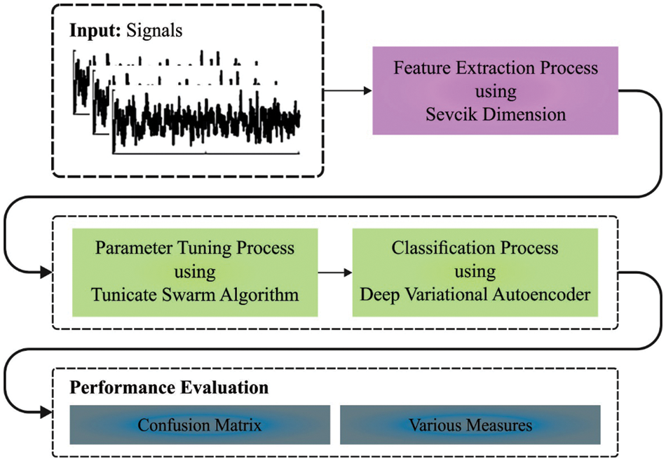
Figure 1: Overall process of the DLIMR-CS technique

3.1 Feature Extraction Using SFD Approach

At first, a set of fractal features is derived from the communication signal using the SFD model. These self-similar dimensions find it difficult to employ the objects that are highly self-similar. So, the box dimensions are utilized to overcome this issue. In a metric space (X,d),A belongs to M non-empty emergency cluster, X. To utilize the box side length of ε, a minimal value N(A,ε) is required for the boxes to cover A as defined below.

N(A,ε)={M:A⊂∑i=1MN(xi,ε)}(1)

where x1,x2,…xM signify the diverse points of X. When ε moves towards 0, the box dimensions are rewritten as follows.

Db=limε→0InN(A,ε)In(1/ε)(2)

Consider a signal with a series of points (xi,yi) and the length of the signal is considered to be N. In this case, the standardization of the signals takes place using Eq. (3) [25]:

xi∗=xi−xminxmax−xmin,yi∗=yi−minymax−ymin(3)

xmin,ymin represent the minimal values between xjandyj. xmax, ymax represent the maximal values between xjandyj. Then, a Sevcik fractal dimension D is defined herewith.

D=1+ ln(L)+ ln(2) ln[2×(N−1)](4)

where L indicates the length of the waveform provided below.

L=∑i=0N−2(yi+1∗−yi∗)2+(xi+1∗−xi∗)2(5)

3.2 Modulation Recognition Using DVAE Model

In this stage, the extracted features are fed into the DVAE model for the classification of different kinds of digitally-modulated signals [26]. With regards to low-dimension embedding achieved by the autoencoder (AE) method, the DVAE network establishes a probabilistic take from the Hidden Variable (HV) space that is optimum to define the salient features of the multi-variate geochemical information. The basic drive of the DVAE model is to utilize the HV z for characterizing the distribution of the original dataset, X ={xi}i=1N. It can be considered that the conditional distribution of HVs z is focused on the Gaussian distribution. As per this model, HV z that fulfills the Gaussian distribution, creates the data and fulfills some of the distribution with NN.

Through the optimization of the created parameter θ, HV z creates a data set X^={xi^}i=1N which is similar to that of the original data, X ={xi}i=1N. This determines the value that is required to maximize the marginal likelihood, pθ(x):

pθ(x)=∫pθ(z)pθ(x|z)dz,withz∼N(0,I)(6)

Since the true posterior density pθ(z|x) cannot be tracked, the DVAE model presents a detection process qϕ(z|x) to resolve this issue and approximate the undefined true posterior pθ(z|x). The DVAE model measures the similarity between the detection process qϕ(z|x) and the true posterior distribution pθ(z|x) with the help of Kullback-Leibler (KL) divergence.

logpθ(x(i))=DKL(qϕ(z|x(i))||pθ(z|x(i)))+L(ϑ,∅;x(i))(7)

Since KL divergence is continuously superior to 0, logpθ(x(i))≥L(θ,p;x(i)).

This equation L(θ,(p;x(i)) denotes the (variational) Lower Bound (LB) on the marginal probability of the data point i which is formulated as follows.

L(θ,(ϕ;x(i))=−DKL(qϕ(z|x(i))‖pθ(z))+Eqϕ(z|(i))[logpθ(x(i)|z)](8)

For the optimization of log pθ(x), the variational LB on the marginal likelihood finds the entirely-optimized objective of the DVAE model. The primary term, on the right side of the Eq. (8), is equivalent to the regularized term, whereas the secondary term is a negative reconstruction error in AE parlance. Thus, qϕ(z|x(i)) is signified as a probabilistic encoder with a variational parameter (ϕ,andpθ(x(i)|z) and is defined as probabilistic decoding with a generation parameter, ϕ. The conditional distribution pθ(x(i)|z) is usually separated into two cases such as Bernoulli and Gaussian distributions. In this case, the input data of the networks are multi-variate geochemical data in nature compared to the binary data, the distribution of pθ(x(i)|z) is considered to be Gaussian.

Then, it can compute the stochastic gradient variational Bayes estimator of the variational LB L(θ,ϕ,x(i)). Then, the detection process qϕ(z|x(i)) is presented based on the re-parameterization approach. Assume z as a continuous arbitrary variable and z∼qϕ(z|x(i)) as a conditional distribution function with an overview of an auxiliary noise variable ε∼p(ε). p(ε) is a known marginal probability distribution. Then, the distribution transformation is executed on qϕ(z|x(i)) outcomes from z~=gϕ(ε,x(i)). While it can be assumed that qϕ(z|x(i)) fulfills a Gaussian distribution and p(z)=N(z;0,I), if the calculation is qϕ(z|x(i))=N(z;u,σ2I), then the regularization term is calculated as follows.

−DKL(qϕ(z|x(i))||p(z))=12∑j=1j(1+log(σ(i)2)−u(i)2−σ(i)2)(9)

whereas j refers to the dimension of z. If Monte Carlo estimation is used to resolve the reconstruction team, then the following equation is attained.

Eqϕ(z|(i))x[logpθ(x(i)|z)=1L∑l=1Llog(p(x(i)|z(i,j))))(10)

Based on the rule of DVAE model, the data reconstruction gets reduced and the root cause of the exceptions is evaluated.

The whole method is trained using normal instances (non-deposits data). So, if the method receives a geochemical anomaly instance in testing data, both encoding as well as decoding of the method depict a superior reconstruction probability between the recreated data of the z and its original data.

3.3 Parameter Optimization Using TSA

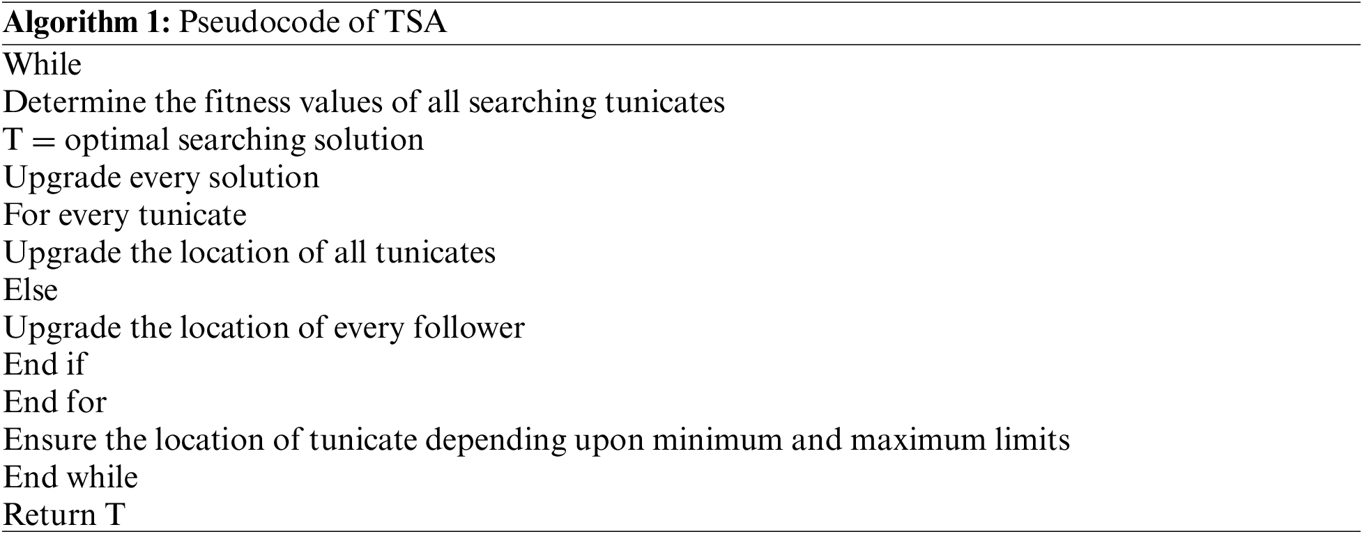
Finally, the TSA model is employed for fine-tuning the parameters involved in the DVAE model which consequently results in the enhanced recognition performance. TSA is a bio-inspired optimization technique. It was originally inspired from the swarming nature of the marine tunicates and its respective jet propulsion during navigation and foraging processes [27]. In TSA, the Tunicate Population (PT) swarming is employed to identify an optimal Food Source (FS) i.e., fitness function. At the time of swarming, a tunicate updates its location based on the initial optimal tunicate position which is saved and updated during all the iterations. The TSA method starts, when the tunicate population undergoes random initialization by considering the permissible limits of the control parameters. The control parameter dimensions contain a tunicate (T), which is primarily generated using Eq. (11):

Tn(m)=Tnmin+r.(Tnmax−Tnmin)∀m∈PTsize&n∈Dim(11)

Here, T(m) represents the location of the tunicate (m); n denotes every control parameter; r indicates an arbitrary number in the interval of [0, 1]; PTsize implies the number of tunicates in a population; and Dim indicates the control variable dimensions. The upgrade procedure of the tunicate location is represented in Eq. (12):

Tn(m)=Tn∗(m)+Tn(m−1)2+c1,∀m∈PTsize&n∈Dim(12)

where, T∗ indicates the upgraded location of the mth tunicate using Eq. (13); T(m − l) implies the neighboring tunicate; and c1 represents an arbitrary number in the interval of [0,1].

Tn∗(m)={SF+A.|SF−rand.Tn(m)|ifrand≥0.5SF−A.|SF−rand.Tn(m)|ifrand<0.5(13)

Here, SF denotes the location of the optimal tunicate in the entire population; A denotes an arbitrary vector that is used to avoid conflict among the tunicates as defined below [28].

A=c2+c3−2c1VTmm˙+c1(VT max −VTmm˙)(14)

Here, c1, c2 and c3 denote the arbitrary numbers in the interval of [0, 1]; VTmm˙ and VTax represent the premier and subordinate speeds in the production of social interactivity. Fig. 2 shows the flowchart of the TSA procedure.

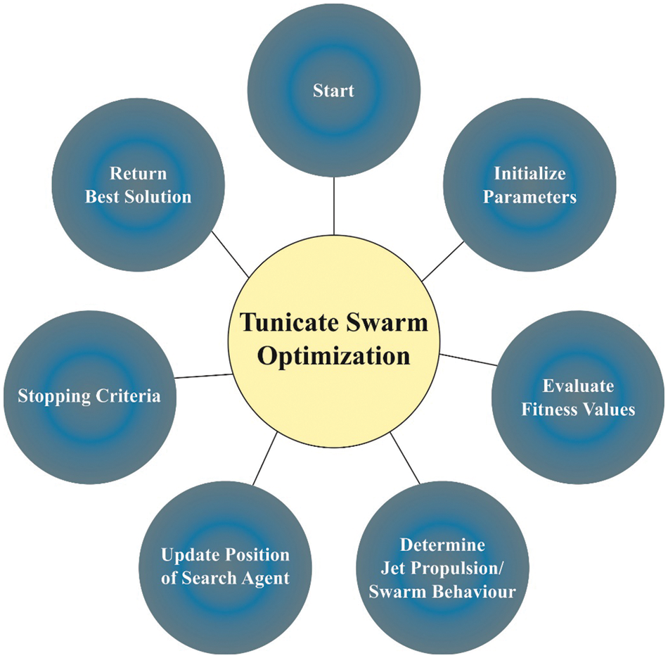
Figure 2: Flowchart of TSA

The TSA system develops a Fitness Function (FF) to achieve enhanced classification outcomes. It defines a positive integer to demonstrate the optimum performance of the candidate results. In this case, a minimum classifier error rate is regarded as the FF as provided in Eq. (15).

fitness (xi)=Classifier Error Rate (xi)

=number of misclassified modulation signalsTotal number of modulation signals*100(15)

4  Performance Validation

In this section, the proposed DLIMR-CS model was experimentally validated in terms of modulation recognition. Table 1 and Fig. 3 illustrate the fractal features offered by distinct communication signals.

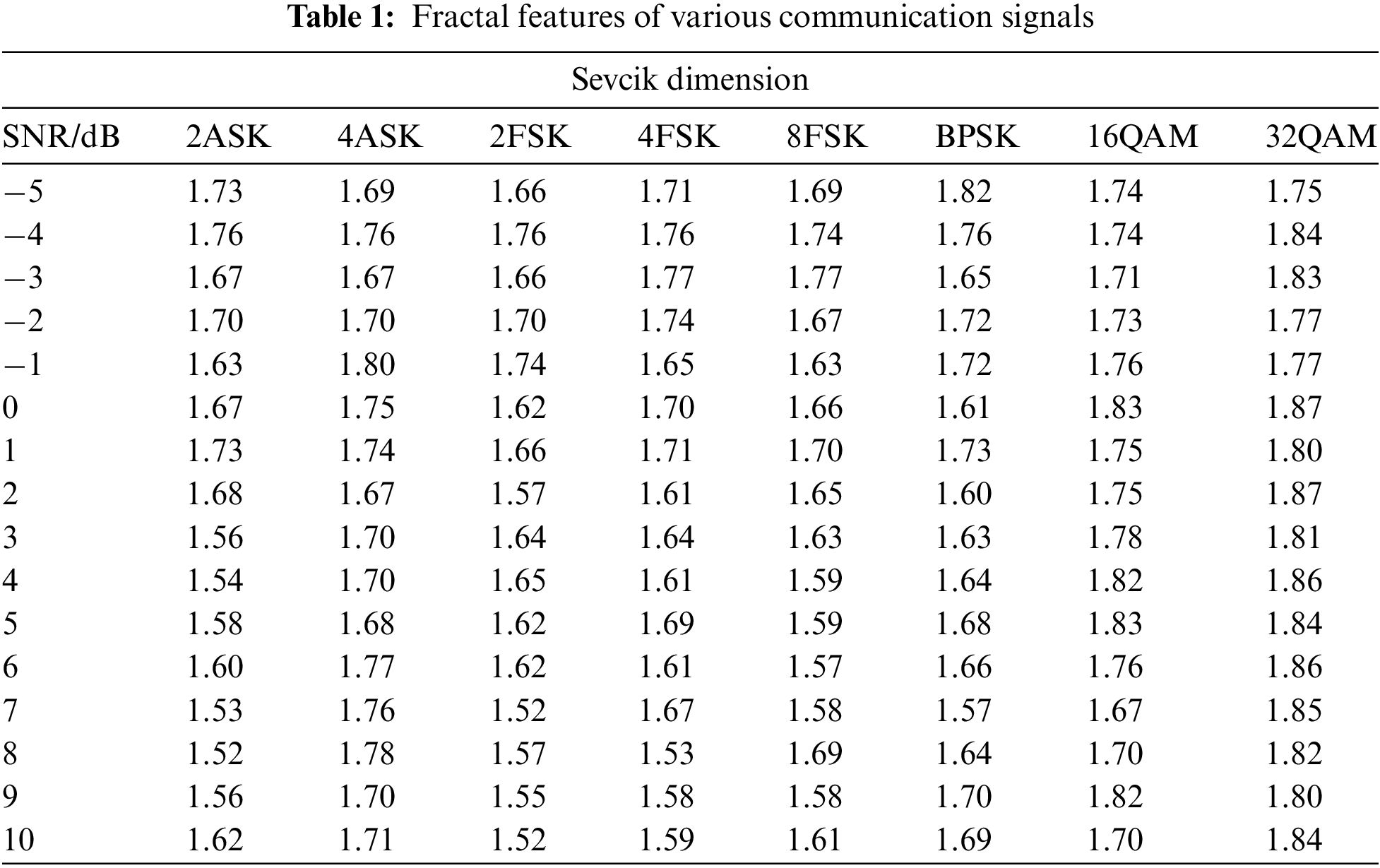
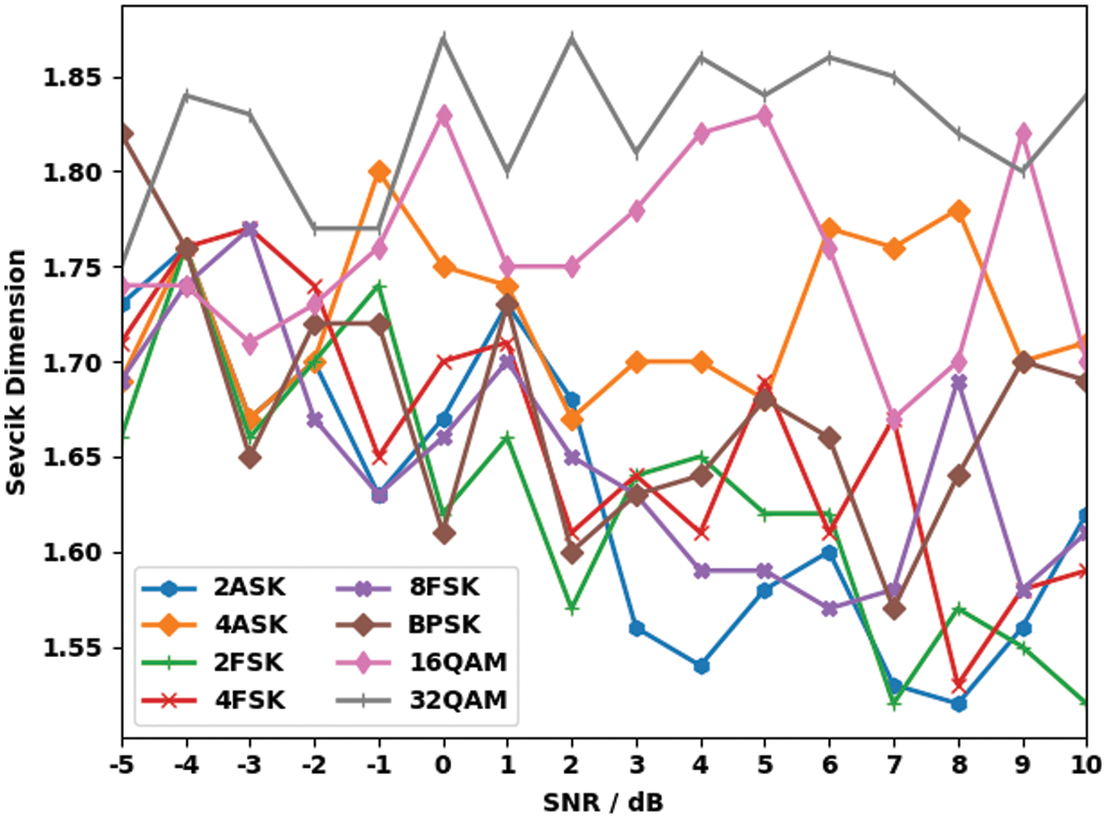
Figure 3: Fractal features of various communication signals

Fig. 4 demonstrates the confusion matrix generated by the DVAE model on 70% training (TRS) dataset under different classes such as Amplitude-shift keying (ASK), frequency-shift keying (FSK) and Quadrature Amplitude Modulation (QAM). The figure indicates that the DVAE model recognized 141 samples as 2ASK, 131 samples as 4ASK, 139 samples as 2FSK, 139 samples as 4FSK, 140 samples as BFSK, 138 samples as BPSK, 138 samples as 16QAM and 135 samples as 32QAM respectively.

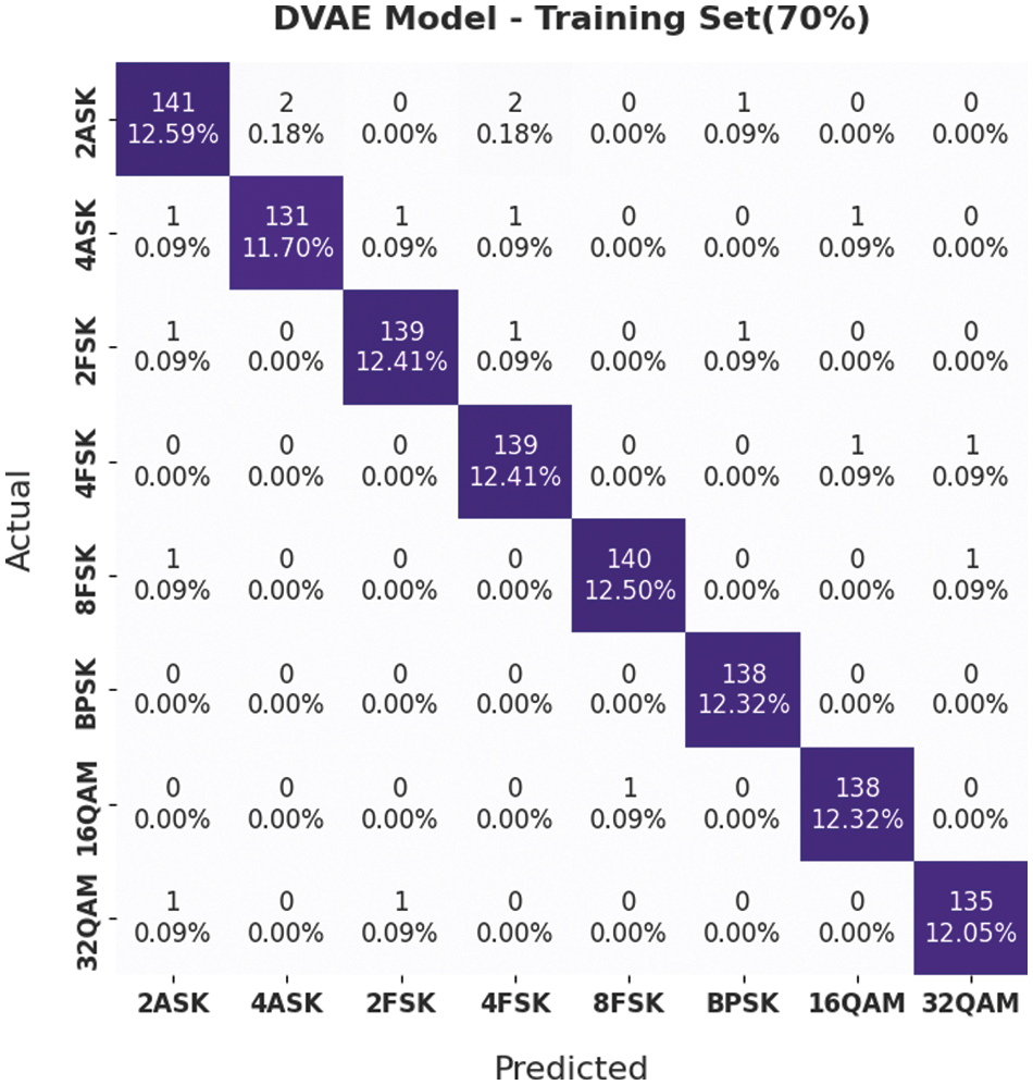
Figure 4: Confusion matrix of the DVAE technique on 70% of TRS dataset

Fig. 5 depicts the confusion matrix of the DVAE technique on 30% of testing (TSS) dataset. The figure infers that the DVAE model classified 53 samples under 2ASK, 64 samples under 4ASK, 58 samples under 2FSK, 57 samples under 4FSK, 58 samples under BFSK, 62 samples under BPSK, 61 samples under 16QAM and 63 samples under 32QAM respectively.

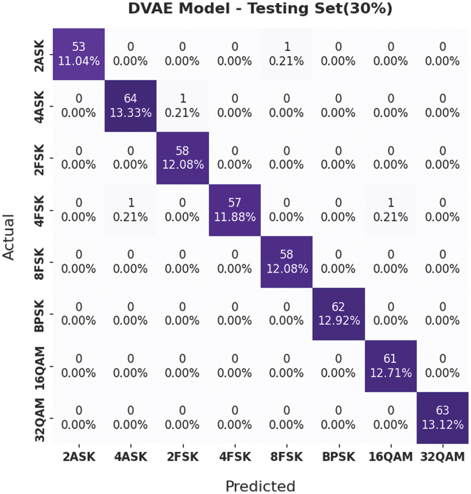
Figure 5: Confusion matrix of the DVAE technique on 30% of TSS dataset

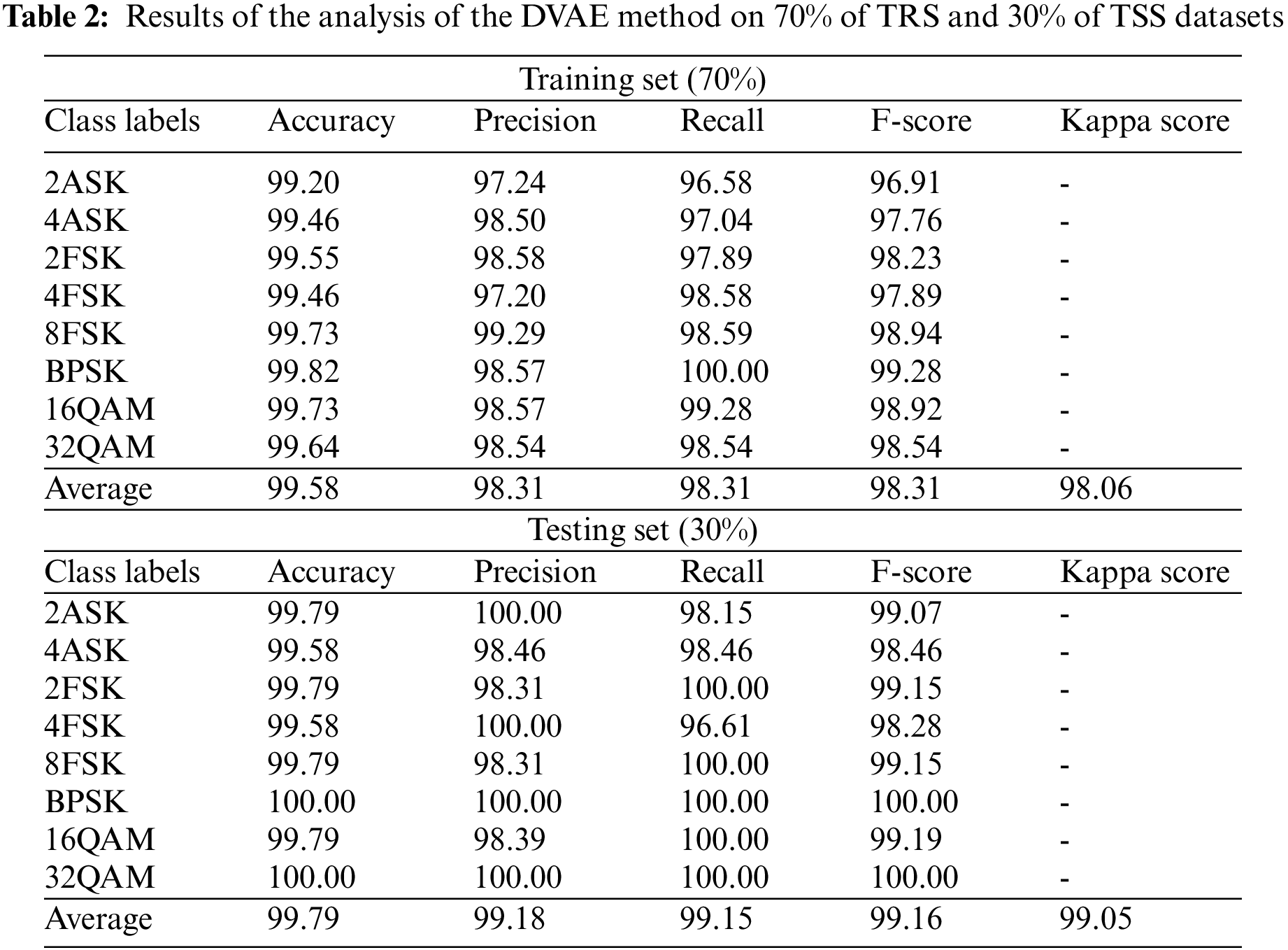
Table 2 reports the MR outcomes achieved by the DVAE model on 70% of TRS and 30% of TSS datasets. The experimental values highlight that the DVAE model achieved effectual MR outcomes. For instance, with 70% of TRS, the DVAE model offered an average accuy of 99.58%, precn of 98.31%, recal of 98.31%, Fscore of 98.31% and a kappa of 98.06%. Besides, with 30% of TSS, the DVAE approach achieved an average accuy of 99.79%, precn of 99.18%, recal of 99.15%, Fscore of 99.16% and a kappa of 99.05%.

Both Training Accuracy (TA) and Validation Accuracy (VA) values, attained by the DVAE model on test data, are illustrated in Fig. 6. The experimental outcomes imply that the DVAE model gained the maximum TA and VA values, whereas VA values were higher than TA values.

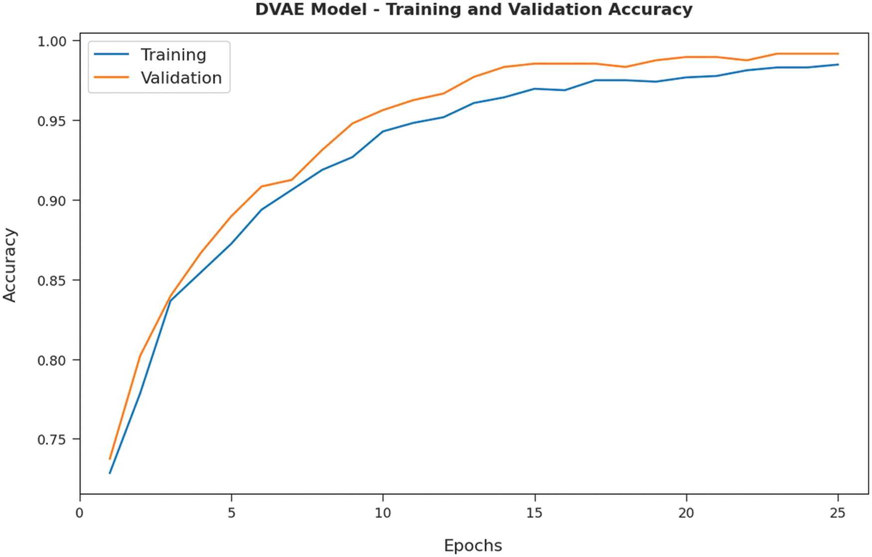
Figure 6: TA and VA analyses results of the DVAE technique

Both Training Loss (TL) and Validation Loss (VL) values, achieved by the DVAE approach on test data, are established in Fig. 7. The experimental outcomes infer that the DVAE model accomplished the least TL and VL values, while the VL values were lesser compared to TL values.

Figure 7: TL and VL analyses results of the DVAE technique

Fig. 8 showcases the confusion matrix of the proposed DLIMR-CS model on 70% of TRS dataset. The figure exposes that the proposed DLIMR-CS model recognized 142 samples as 2ASK, 132 samples as 4ASK, 142 samples as 2FSK, 140 samples as 4FSK, 142 samples as BFSK, 138 samples as BPSK, 139 samples as 16QAM and 134 samples as 32QAM respectively.

Figure 8: Confusion matrix of the proposed DLIMR-CS technique on 70% of TRS dataset

Fig. 9 portrays the confusion matrix of the proposed DLIMR-CS model on 30% of TSS. The figure indicates that the proposed DLIMR-CS technique classified 54 samples under 2ASK, 64 samples under 4ASK, 58 samples under 2FSK, 59 samples under 4FSK, 58 samples under BFSK, 62 samples under BPSK, 61 samples under 16QAM and 62 samples under 32QAM respectively.

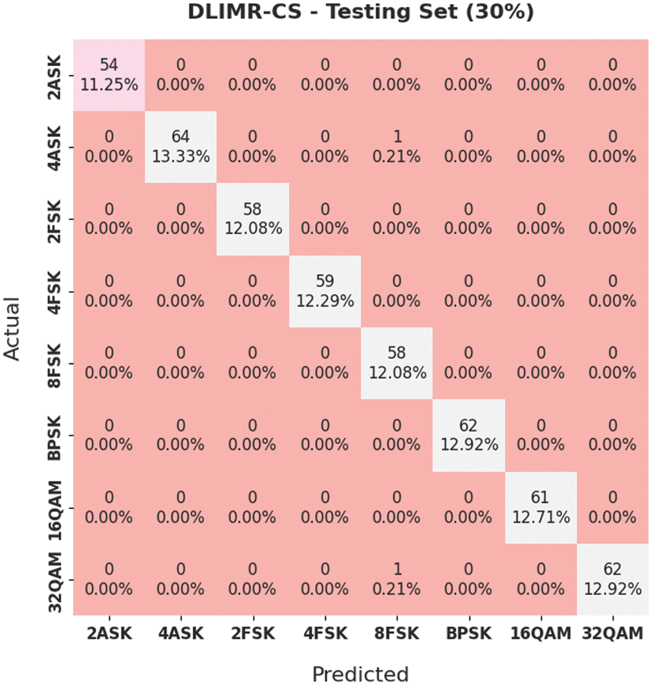
Figure 9: Confusion matrix of the DLIMR-CS technique on 30% of TSS dataset

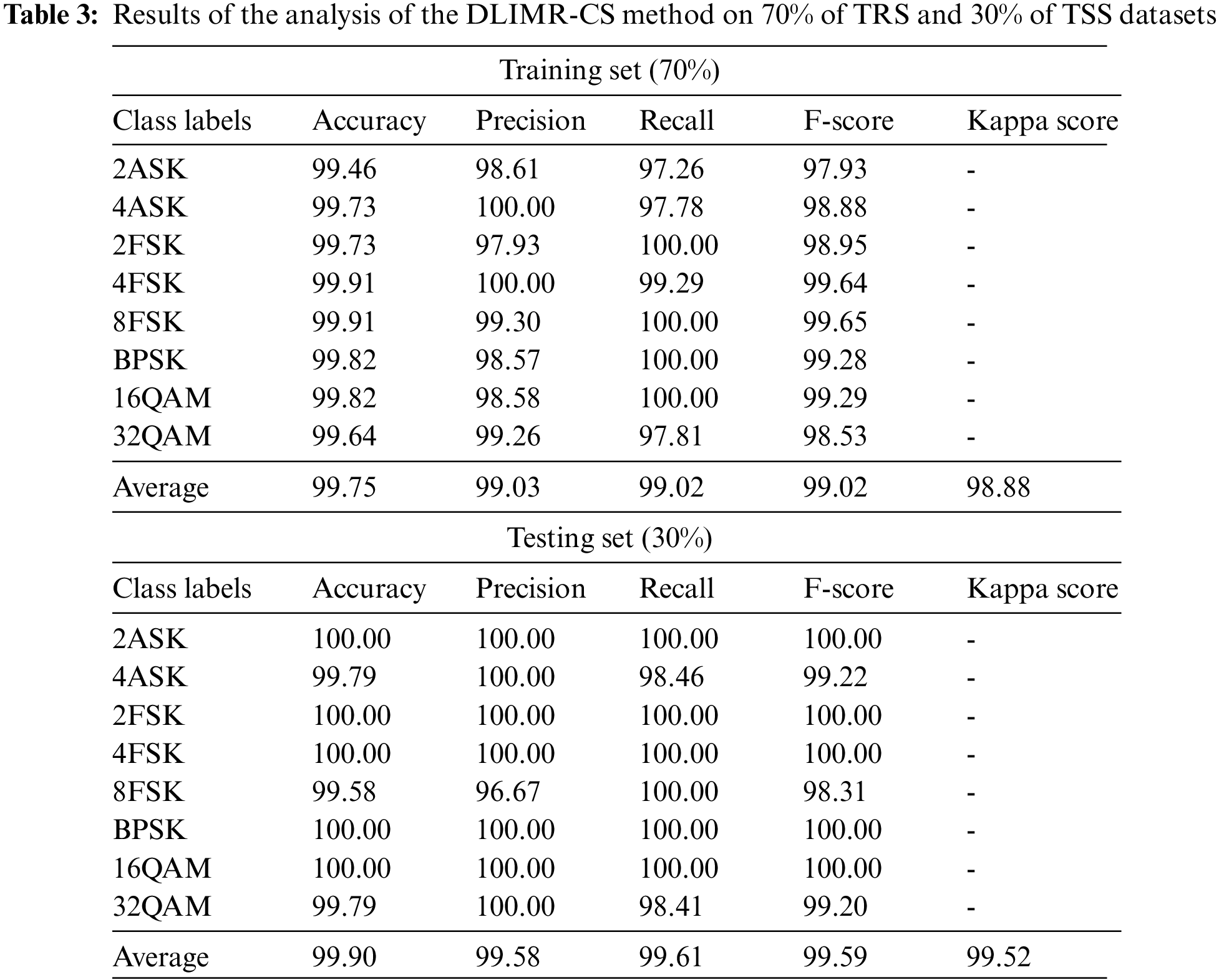
Table 3 portrays the MR outcomes of the proposed DLIMR-CS model on 70% of TRS and 30% of TSS datasets. The experimental values highlight that the proposed DLIMR-CS model achieved effectual MR outcomes on both the aspects. For instance, with 70% of TRS, the DLIMR-CS technique achieved an average accuy of 99.75%, precn of 99.03%, recal of 99.02%, Fscore of 99.88% and a kappa of 98.06%. At last, with 30% of TSS, the proposed DLIMR-CS approach obtained an average accuy of 99.90%, precn of 99.58%, recal of 99.61%, Fscore of 99.59% and a kappa of 99.52%.

Both TA and VA values, attained by the proposed DLIMR-CS approach on test data, are shown in Fig. 10. The experimental outcomes imply that the proposed DLIMR-CS technique gained the maximal TA and VA values, whereas VA values were higher than the TA values.

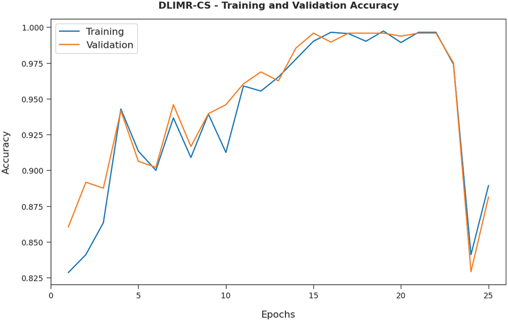
Figure 10: TA and VA analyses results of the DLIMR-CS technique

Both TL and VL values, achieved by the proposed DLIMR-CS system on test data, are established in Fig. 11. The experimental outcomes infer that the proposed DLIMR-CS technique accomplished the least TL and VL values, whereas VL values were lesser than the TL values.

Figure 11: TA and VA analyses results of the DLIMR-CS technique

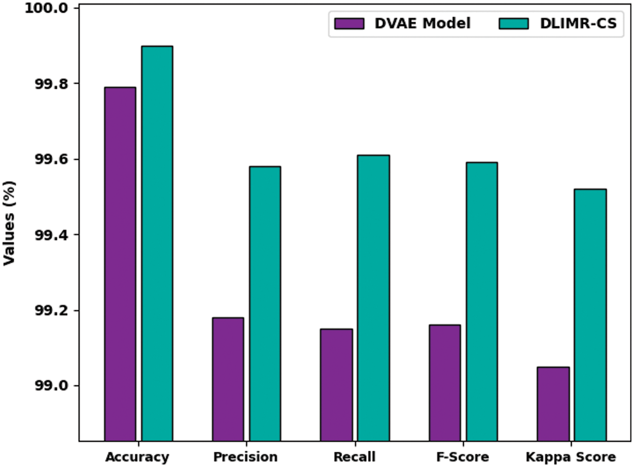
Figure 12: Average analysis results of the DLIMR-CS technique under different measures

Finally, a detailed comparative examination was conducted between the proposed DLIMR-CS model and other recent models in terms of Recognition Rate (RR) and the results are provided in Fig. 13 [29]. The experimental results indicate that both KNN and GR models achieved the least performance with minimal RR values. Followed by, the NN model attempted to yield a slightly enhanced RR.

Figure 13: Recognition rate under various SNRs

In line with this, the RF model managed to exhibit a reasonable RR. Though the DVAE model produced a considerable performance, the presented DLIMR-CS model achieved a maximum RR under distinct SNR levels. Therefore, the presented DLIMR-CS model is found to be superior to other models on MR performance under varying SNR levels.

Table 4 and Fig. 12 report the overall MR outcomes of DVAE and DLIMR-CS models. The experimental outcomes infer that the DVAE model gained an average accuy of 99.79%, precn of 99.18%, recal of 99.15%, Fscore of 99.16% and a kappa of 99.05%. Also, the proposed DLIMR-CS model accomplished an average accuy of 99.90%, precn of 99.58%, recal of 99.61%, Fscore of 99.59% and a kappa of 99.52%.

5  Conclusion

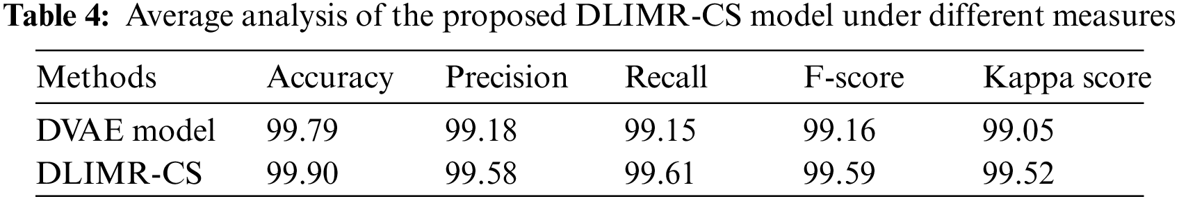
In this study, a novel DLIMR-CS model has been developed for modulation recognition in next-generation networks. The presented DLIMR-CS model primarily utilizes the SFD model for the extraction of the fractal features. In addition, the extracted features are fed into the DVAE model for proficient recognition of the modulated signals. Finally, the TSA approach is employed for the parameter optimization of the DVAE model. A wide range of simulations was conducted to highlight the enhanced performance of the proposed DLIMR-CS model. The experimental outcomes infer the superior recognition rate of the DLIMR-CS model over other state-of-the-art methods under different evaluation parameters. Therefore, the presented DLIMR-CS model can be employed for effective detection and classification of the modulated signals. In the future, hybrid DL models can be involved to improve the overall modulation recognition performance.

Funding Statement: The author received no specific funding for this study.

Conflicts of Interest: The author declares that they have no conflicts of interest to report regarding the present study.

References

 1.  T. Sharma, A. Chehri and P. Fortier, “Review of optical and wireless backhaul networks and emerging trends of next-generation 5G and 6G technologies,” Transactions on Emerging Telecommunications Technologies, vol. 32, no. 3, pp. e4155, 2021. [Google Scholar]

 2.  B. T. Maharaj and B. S. Awoyemi, “The role of cognitive radio networks in fifth-generation communication and beyond,” in Developments in Cognitive Radio Networks, Cham: Springer, pp. 209–217, 2022. [Google Scholar]

 3.  X. Li, F. Dong, S. Zhang and W. Guo, “A survey on deep learning techniques in wireless signal recognition,” Wireless Communications and Mobile Computing, vol. 2019, pp. 1–12, 2019. [Google Scholar]

 4.  X. Zhang, J. Sun and X. Zhang, “Automatic modulation classification based on novel feature extraction algorithms,” IEEE Access, vol. 8, pp. 16362–16371, 2020. [Google Scholar]

 5.  A. M. Hilal, J. S. Alzahrani, I. Abunadi, N. Nemri, F. N. Al-Wesabi et al., “Intelligent deep learning model for privacy preserving IIoT on 6G environment,” Computers, Materials & Continua, vol. 72, no. 1, pp. 333–348, 2022. [Google Scholar]

 6.  D. Zhang, W. Ding, B. Zhang, C. Xie, H. Li et al., “Automatic modulation classification based on deep learning for unmanned aerial vehicles,” Sensors, vol. 18, no. 3, pp. 924, 2018. [Google Scholar]

 7.  C. Weber, M. Peter and T. Felhauer, “Automatic modulation classification technique for radio monitoring,” Electronics Letters, vol. 51, no. 10, pp. 794–796, 2015. [Google Scholar]

 8.  A. Abdelmutalab, K. Assaleh and M. El-Tarhuni, “Automatic modulation classification based on high order cumulants and hierarchical polynomial classifiers,” Physical Communication, vol. 21, pp. 10–18, 2016. [Google Scholar]

 9.  F. N. Al-Wesabi, M. Obayya, M. Hamza, J. S. Alzahrani, D. Gupta et al., “Energy aware resource optimization using unified metaheuristic optimization algorithm allocation for cloud computing environment,” Sustainable Computing: Informatics and Systems, vol. 35, pp. 100686, 2022. [Google Scholar]

10. B. Jdid, K. Hassan, I. Dayoub, W. H. Lim and M. Mokayef, “Machine learning based automatic modulation recognition for wireless communications: A comprehensive survey,” IEEE Access, vol. 9, pp. 57851–57873, 2021. [Google Scholar]

11. S. Peng, S. Sun and Y. D. Yao, “A survey of modulation classification using deep learning: Signal representation and data preprocessing,” IEEE Transactions on Neural Networks and Learning Systems, pp. 1–19, 2021. https://doi.org/10.1109/TNNLS.2021.3085433. [Google Scholar]

12. T. Wang, Y. Hou, H. Zhang and Z. Guo, “Deep learning based modulation recognition with multi-cue fusion,” IEEE Wireless Communications Letters, vol. 10, no. 8, pp. 1757–1760, 2021. [Google Scholar]

13. L. Weng, Y. He, J. Peng, J. Zheng and X. Li, “Deep cascading network architecture for robust automatic modulation classification,” Neurocomputing, vol. 455, pp. 308–324, 2021. [Google Scholar]

14. J. C. Clement, N. Indira, P. Vijayakumar and R. Nandakumar, “Deep learning based modulation classification for 5G and beyond wireless systems,” Peer-to-Peer Networking and Applications, vol. 14, no. 1, pp. 319–332, 2021. [Google Scholar]

15. S. Hanna, C. Dick and D. Cabric, “Signal processing-based deep learning for blind symbol decoding and modulation classification,” IEEE Journal on Selected Areas in Communications, vol. 40, no. 1, pp. 82–96, 2022. [Google Scholar]

16. S. Chang, S. Huang, R. Zhang, Z. Feng and L. Liu, “Multitask-learning-based deep neural network for automatic modulation classification,” IEEE Internet of Things Journal, vol. 9, no. 3, pp. 2192–2206, 2022. [Google Scholar]

17. X. R. Jiang, H. Chen, Y. D. Zhao and W. -Q. Wang, “Automatic modulation recognition based on mixed-type features,” International Journal of Electronics, vol. 108, no. 1, pp. 105–114, 2021. [Google Scholar]

18. K. Chen, S. Zhang, L. Zhu, S. Chen and H. Zhao, “Modulation recognition of radar signals based on adaptive singular value reconstruction and deep residual learning,” Sensors, vol. 21, no. 2, pp. 449, 2021. [Google Scholar]

19. K. Liu, W. Gao and Q. Huang, “Automatic modulation recognition based on a dcn-bilstm network,” Sensors, vol. 21, no. 5, pp. 1577, 2021. [Google Scholar]

20. J. Chen, H. Cui, S. Miao, C. Wu, H. Zheng et al., “FEM: Feature extraction and mapping for radio modulation classification,” Physical Communication, vol. 45, pp. 101279, 2021. [Google Scholar]

21. S. Wei, Q. Qu, X. Zeng, J. Liang, J. Shi et al., “Self-attention bi-LSTM networks for radar signal modulation recognition,” IEEE Transactions on Microwave Theory and Techniques, vol. 69, no. 11, pp. 5160–5172, 2021. [Google Scholar]

22. J. N. Njoku, M. E. M. Cayamcela and W. Lim, “CGDNet: Efficient hybrid deep learning model for robust automatic modulation recognition,” IEEE Networking Letters, vol. 3, no. 2, pp. 47–51, 2021. [Google Scholar]

23. A. Jagannath and J. Jagannath, “Multi-task learning approach for automatic modulation and wireless signal classification,” in ICC 2021-IEEE Int. Conf. on Communications, Montreal, QC, Canada, pp. 1–7, 2021. [Google Scholar]

24. C. Hou, Y. Li, X. Chen and J. Zhang, “Automatic modulation classification using KELM with joint features of CNN and LBP,” Physical Communication, vol. 45, pp. 101259, 2021. [Google Scholar]

25. Y. S. Liang, “Fractal dimension of Riemann-Liouville fractional integral of 1-dimensional continuous functions,” Fractional Calculus and Applied Analysis, vol. 21, no. 6, pp. 1651–1658, 2018. [Google Scholar]

26. Z. Luo, Y. Xiong and R. Zuo, “Recognition of geochemical anomalies using a deep variational autoencoder network,” Applied Geochemistry, vol. 122, pp. 104710, 2020. [Google Scholar]

27. S. Kaur, L. K. Awasthi, A. L. Sangal and G. Dhiman, “Tunicate swarm algorithm: A new bio-inspired based metaheuristic paradigm for global optimization,” Engineering Applications of Artificial Intelligence, vol. 90, pp. 103541, 2020. [Google Scholar]

28. T. Fetouh and A. M. Elsayed, “Optimal control and operation of fully automated distribution networks using improved tunicate swarm intelligent algorithm,” IEEE Access, vol. 8, pp. 129689–129708, 2020. [Google Scholar]

29. C. T. Shi, “Signal pattern recognition based on fractal features and machine learning,” Applied Sciences, vol. 8, no. 8, pp. 1327, 2018. [Google Scholar]