Lightning Search Algorithm with Deep Transfer Learning-Based Vehicle Classification

1  Introduction

The advent of Machine Learning (ML) techniques and its implementation in multiple domains for problem solving, replacing statistical methods have transformed to the thresholds to higher levels with the application of these novel techniques [1]. Transportation systems have been positively influenced with the development of ML techniques, specifically from Intelligent Transportation Systems (ITS). With the expansion of big data and computational methods like Graphical Processing Units (GPUs), a particular class of ML named Deep Learning (DL) gained familiarity among the researchers. The ability of DL methods to handle huge volumes of data and extract knowledge from complicated systems are leveraged to achieve powerful and feasible solutions in the field of ITS [2]. Researchers make use of different DL networks in framing the issues faced in network, for instance resolving an issue with one of the Neural Network (NN) methods [3,4]. Several innovative solutions have been proposed and validated for traffic signal control to achieve optimum traffic management, increased transportation security through investigation sensor nodes, traffic rerouting model, health observation of transportation structure, and other such issues. These issues have been overcome with the help of robust techniques in the field of transportation engineering [5].

With an exponential production of vehicles across the globe, vehicle classification models serve a crucial role in different areas such as the advancement of ITS in traffic flow control systems, automatic highway toll collection, and perception in self-driving vehicles [6,7]. In early research works, loop and laser induction sensors-related methodologies were suggested for classification of the vehicle types [8]. Such sensors are fixed under road pavement for collection and analysis of the data to extract appropriate data with regards to vehicles. But, it is important to know that the stability and accuracy of such methods have been affected due to unfavourable weather conditions and damage occurred in road pavement [9,10]. Essentially, computer vision-related classification system is a two-step procedure; firstly, handcrafted extraction methodologies are used to obtain visual characteristics from input visual frames [11].

Secondly, ML classifiers are well-trained on the derived characteristics to classify group related data [12]. These algorithms accomplish the objective properly in specific controlled environments and are very comfortable with regards to maintenance and installation over the prevailing laser and inductive-related schemes. Further, these techniques are well-trained on the confined handcrafted characteristics that are derived from minor dataset. However, there is a need exists to have wide and in-depth knowledge to maintain and achieve precise period situation [13]. In recent years, DL-related Feature Selection (FS) and classification techniques have been launched which show better adaptability and applicability than the conventional classification methods. Convolutional Neural Network (CNN)-related classification algorithms reached high accuracy on large scale image dataset because of its sophisticated infrastructure.

The current study develops a Lightning Search Algorithm with Deep Transfer Learning based Vehicle Classification Model for ITS abbreviated as LSADTL-VCITS model. The key objective of the presented LSADTL-VCITS is to automatically detect and classify the types of vehicles. To accomplish this, the presented LSADTL-VCITS model initially employs You Only Look Once (YOLO)-v5 object detector with Capsule Network (CapsNet) as a baseline model. In addition, LSADTL-VCITS model applies LSA with Multilayer Perceptron (MLP) for detection and classification of the vehicles. The performance of the proposed LSADTL-VCITS model was experimentally validated utilizing benchmark dataset and the outcomes were examined under several measures.

2  Related Works

Butt et al. [14] suggested a CNN-related vehicle classification algorithm to improve the strength of vehicle classification in real-time applications. Previously, pre-trained Inception-v3, AlexNet, Visual Geometry Group (VGG), ResNet, and GoogleNet were fine-tuned over self-constructed vehicle datasets so as to evaluate its execution efficiency in terms of convergence and accuracy. ResNet architecture was found to have performed well, based on its superior performance, after inclusion of a new classification block in its network. In literature [15], a DL-related traffic safety solution was suggested for a combination of manual and autonomous vehicle classification system in 5G-enabled ITS. In this method, the ending intention probability was acquired by combining the mean rule in decision layer. The authors in the study conducted earlier [16] designed a target detection system based on DL methods, especially CNN and NN modelling. Having been designed on the scrutiny of conventional Haar-like vehicle recognition system, this study suggested a vehicle recognition system related to CNN with Fused Edge features (FE-CNN).

Ashraf et al. [17] provided a DL-related Intrusion Detection System (IDS) for ITS to identify the suspicious activities in Vehicles to Infrastructure (V2I) networks, In-Vehicles Networks (IVN), and Vehicles to Vehicle (V2V) transmissions. A DL architecture-related Long Short Term Memory (LSTM) Autoencoder system was developed earlier to identify intrusions in central network gateways of Autonomous Vehicles (AVs). Tsai et al. [18] suggested an optimized vehicle classification and detection technique on the basis of DL technology for intellectual transportation applications. In this study, the authors enhanced the CNN infrastructure by fine-tuning the prevailing CNN infrastructure for intelligent transportation applications. Wang et al. [19] recommended a new Rear-end Collision Prediction Mechanism by means of DL technique (RCPM), in which a CNN technique was utilized. In RCPM, the dataset was expanded and smoothed on the basis of genetic theory so as to alleviate class imbalance issue. The pre-processed dataset was classified into testing and training datasets as inputs to train the CNN method.

3  The Proposed Model

In this study, a novel LSADTL-VCITS approach is introduced for identification and classification of vehicles in ITS environment. The presented LSADTL-VCITS model has two stages such as vehicle detection and vehicle classification. At first, YOLO-v5 model is applied for the recognition of vehicles. Secondly, LSA is used with MLP method for the classification of vehicles under distinct classes.

3.1 Vehicle Detection Module

In this study, YOLO-v5 model is applied for the recognition of vehicles. YOLOv5 technique, the state-of-the-art version of YOLO technique, is an established technique known for its breakneck recognition speed and high accuracy. YOLOv5 approach has a recognition speed as low as 2 ms per image on single NVIDIA Tesla v100 [20]. The presented technique needs an input image, identified from chunks which is then integrated into a single image; thus, the YOLOv5 technique is selected as the object recognition technique with superior recognition speed and real-time efficiency. YOLOv5 network method has three important infrastructures such as recognition head, backbone, and feature pyramid network.

The loss function is formulated as follows.

loss=lbox+lcls+lobj,(1)

whereas lbox, lcls, and lobj signify the bounding box regression loss function, classifier loss function, and confidence loss function correspondingly.

Bounding box regression loss function can be determined as given below.

lbox=λcoord∑i=0S2∑j=0BIi,jojbbj(2−wi×hi)

[(xi−x∧ij)2+(yi−y∧ij)2+(wi−w∧ij)2+(hi−h∧ij)2].(2)

Further, classifier loss function is expressed as follows

lcls=λclass∑i=0jS2∑=0BIi,jobj∑C∈c1assespi(c)log⁡(p^l(c)).(3)

Confidence loss function can be calculated as given below

lobj=λnoobj∑i=0jS2∑=0BIi,jnoobj(ci−c∧l)2+λobj∑i=0s2∑j=0BIi,jobj(ci−c∧l)2,(4)

Here, λcoord implies place loss co-efficient, λclass signifies category loss co-efficient, x^, y^ refers to true central co-ordinates of the target, and w^, h^ represent the width and height of the target.

When the anchor box at (i,j) comprises of targets, before the value Ii,jobj is 1; else, the value is 0. pi(c) denotes the type probability of targets, and p^l(c) refers to true value of the categories. The length of 2 is equivalent to the entire number of categories, C.

Besides, CapsNet model is also utilized as the baseline model. CapsNet is conceived from capsules [21] i.e., a collection of neurons in which the activity vector signifies discrete parameters of a particular entity. In addition, the capsule exhibits better resistance to white box adversarial attack compared to standard CNN. This is to ensure that the capsule has the capacity to retain every spatial information. The underlying CapsNet contains a convolution layer, alternative convolution layer named PrimaryCaps layer, and the last layer in the name of DigitCaps layer. CapsNet has one PrimaryCaps layer, one DigitCaps layer, and one convolution layer. Every set of 8 scalars in a feature map tensor constitutes i PrimaryCap. ui signifies the output of i PrimaryCap. u^ specifies the prediction vector viz. input of j final DigitCaps. Wij refers to the weight matrix.

u^i|j=Wijui(5)

Routing, by agreement, might transfer the output of PrimaryCaps to final aps by enhancing or reducing the close relationship between PrimaryCaps and DigitCaps in place of pooling process and then retaining the spatial relationship amongst other object parts. The coupling coefficients amongst the two Caps are increased, when the output is equal. bij indicates a logit of Softmax operation that defines cij coupling coefficient amongst i Caps in layer above and below j Caps in layer, as follows.

cij=exp⁡(bij)Σkexp⁡(bik)′sj=∑iciju^j|i(6)

The vector length sj symbolizes the input of DigitCaps layer and is constraint to one by squash determination to attain the output vj. The inner product of vj and u^ upgrades the log likelihood bij. The most comparable two vectors are, lengthier the vector vj will be. Fig. 1 depicts the framework of CapsNet.

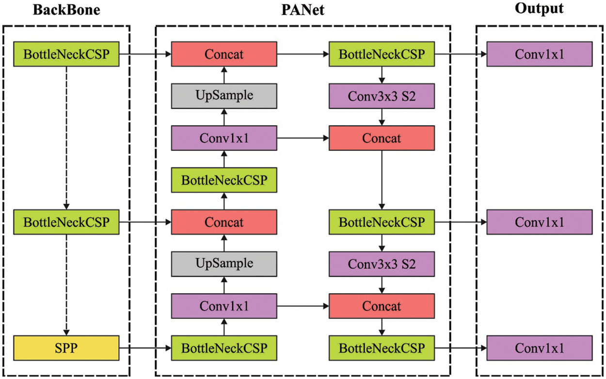
Figure 1: Structure of CapsNet

Varied CapsNet utilizes three level caps layers to learn dissimilar features and focus on multi-dimension vectors. DeepCaps exploits 3-D convolution layers and exceeds the advanced outcome in the region of CapsNet. CapsNet has been extensively applied in several fields. The attention method has accomplished a tremendous growth in the field of CV. It assists the model in emphasizing the relationship amongst regions of images and encompassing long range dependency via image region. SENet uses channel-wise importance to get considered for the technique that places more weight on the network with real significance. GCNet collectively fuses the benefits of Squeeze Excitation (SE) and Non-local blocks to attain better global context blocks.

3.2 Vehicle Classification Module

After vehicle detection process, vehicle classification is carried out using LSA with MLP model. Perceptron is a basic Artificial Neural Network (ANN) architecture based on slight distinct artificial neurons in the name of Threshold Logic Unit (TLU) or the Linear Threshold Unit (LTU) [22]. TLU assesses the weighed amount of the input as follows:

z=w1x1+w2x2+…+wnxn=xτW(7)

Then, a step function is applied for the sum and the outcomes are regarded as output.

hw(x)=step(z)(8)

But, z=xτW. Perceptron is composed of a single layer of TLU linked with all the input values. When the neurons in a layer are connected together, it is called Fully-Connected (FC) layer or a dense layer. The resulting ANN is also known as MLP. In order to train the MLP, Back Propagation training method is applied for automatic computation of the gradients.

In order to adjust the parameters related to MLP approach, LSA is employed. LSA is a metaheuristic approach that simulates the natural phenomenon of lightning [23]. LSA depends upon Step Leader (SL) approach in which the projectiles are considered as individuals and are quicker particles. The primary stage of LSA is to determine the projectile that signifies the population. Conversely, the solution of populations refers to the tip of present SL. There are different phases of LSA exist and the particulars of all of them are provided in the subsequent section.

When a projectile travels in normal criteria within the atmosphere, its kinetic energy gets reduced during collision with atoms and molecules present in the air. The velocity of the projectiles is expressed as follows

vp=[1−(1/1−(v0/c)2−s×Fi/m×c2)−2]−1/2(9)

Here, vp and v0 imply the primary velocity and present velocity of the projectiles correspondingly. c and Fi signify the speed of lights and rate of ionizations respectively. While the rate of ionization can be constant as well. But m stands for mass of the projectiles, and s demonstrates the length of the path. In Eq. (9), it can be experiential that the velocity is dependent upon the mass of projectiles and the place of leader tips. Therefore, both exploration and exploitation of LSA are controlled through the comparative energies of SLS.

SL is another property named ‘forking’ which happens if two symmetrical and simultaneous branches have occurred. Forking is inspired based on two approaches, (1) utilizing the opposite number to represent the design of symmetrical channels in nuclei collision from the subsequent formula:

P¯i=UB+LB−pi(10)

whereas pi and p¯i denote the projectiles and their opposites correspondingly. But, UB and LB signify the restrictions of search space.

A group of three kinds of the projectiles is executed for Transition Projectiles (TP) procedure and it is utilized to construct the First-Step Leader (FSL) population, N. Besides, it can be utilized to create the Space Projectiles (SP) that attempt at determining the place of an optimum leader. Similarly, an individual’s varieties are utilized to build the Lead Projectiles (LP) that signify the entire optimum place, N SL. For clarification, the particulars of all these types are provided subsequently.

Then, the leader tip is created at primary stage, because the ejected projectile is arbitrarily generated in thunder cell with the help of transitions. Therefore, it is signified by creating an arbitrary number in a uniform distribution which is determined using Eq. (11).

f(xT)={1b−afora≤xT≤b0x<aorx>b(11)

Here, a and b denote the restricted searching spaces. xT defines the solution or tip energy (Esl,i) of SL (sli). For the population i.e., N SL (that is, SL=[sl1,sl2,…slN]), a set of N projectiles PT=[p1T,p2T,…,pNT] is desired. Fig. 2 demonstrates the flowchart of LSA.

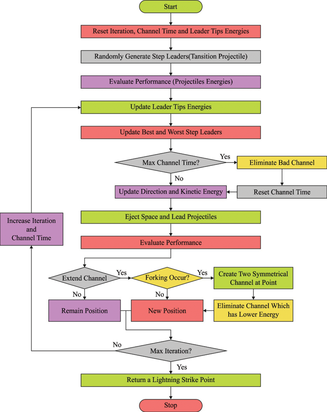
Figure 2: Flowchart of LSA

In LSA, SP is demonstrated as an arbitrary number that is created with the help of exponential distribution as determined herewith.

f(xS)={1μe−xSμxS≥00otherwise(12)

Here, μ refers to the shape of distribution which can be utilized for controlling SP PS=[p1S,p2S,…,pNS] at step+1. The μ for ith SP is determined as the distance between (i.e., piS) and its leader project, pL. In line with this description, the value of piS is updated using the subsequent equation:

pinewS=piS±exprand(μi)(13)

whereas exprand denotes the exponential arbitrary number with shape, μi. In case of piS<0 before exprand is subtracted, Eq. (13) offers a value superior to 0. But, pinewS promises a stepped leader propagation, if the projectile energy EpiS>Esli. In this scenario, it is possible still to achieve an optimum solution. Both piS and sli are extended pinewS and slinew correspondingly, if their equivalent pinewS at step +1 attains the optimum solution. Then, each other (i.e., piS and sl) remains unchanged until the step completes.

With regards to SP, LP gets upgraded to a predictable formula with the help of arbitrary number that is created in normal distribution as given below.

f(xL)=1σnπe−(xL−μ)2/2σ2(14)

whereas σ and μ signify the scale and shape of the distributions correspondingly. The place of LP (p) is upgraded using a normal random number normrand as determined in Eq. (15).

pinewL=pi|±normrand(μL,σL)(15)

LSA approach resolves a Fitness Function (FF) to achieve high classification efficiency. It defines a positive integer so as to signify the optimal efficiency of candidate outcomes. In this case, the minimum classifier error rate is assumed to be the FF as offered in Eq. (16).

fitness(xi)=ClassifierErrorRate(xi)=numberofmisclassifiedvehiclesTotalnumberofvehicles∗100(16)

4  Performance Validation

The current section validates the vehicle classification performance of the proposed LSADTL-VCITS model using Veri dataset [24]. The dataset holds images under six classes namely bus, Multi-Purpose Vehicle (MPV), pickup, sedan, truck, and van. The details, related to the dataset, are shown in Table 1.

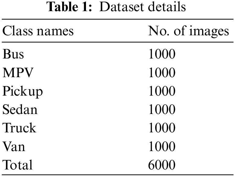
Fig. 3 illustrates the confusion matrices generated by the proposed LSADTL-VCITS model on the applied test dataset. The figure indicates that the proposed LSADTL-VCITS approach gained effectual outcomes under all classes. On 70% of training (TR) data, LSADTL-VCITS model categorized 654 images under bus, 700 images under MPV, 684 images under pickup, 673 images under Sedan, 683 images under truck, and 674 images under van class respectively. Also, on 30% of testing (TS) data, the proposed LSADTL-VCITS system categorized 332 images as bus, 284 images as MPV, 287 images as pickup, 295 images as Sedan, 276 images as truck, and 284 images as van respectively. In addition to these, on 90% of TR data, the presented LSADTL-VCITS approach classified 907 images under bus, 888 images under MPV, 894 images under pickup, 892 images under sedan, 896 images under truck, and 900 images under van respectively. At last, on 10% of TS data, the proposed LSADTL-VCITS algorithm segregated 90 images into bus, 110 images into MPV, 104 images into pickup, 100 images into Sedan, 100 images into truck, and 94 images into van classes correspondingly.

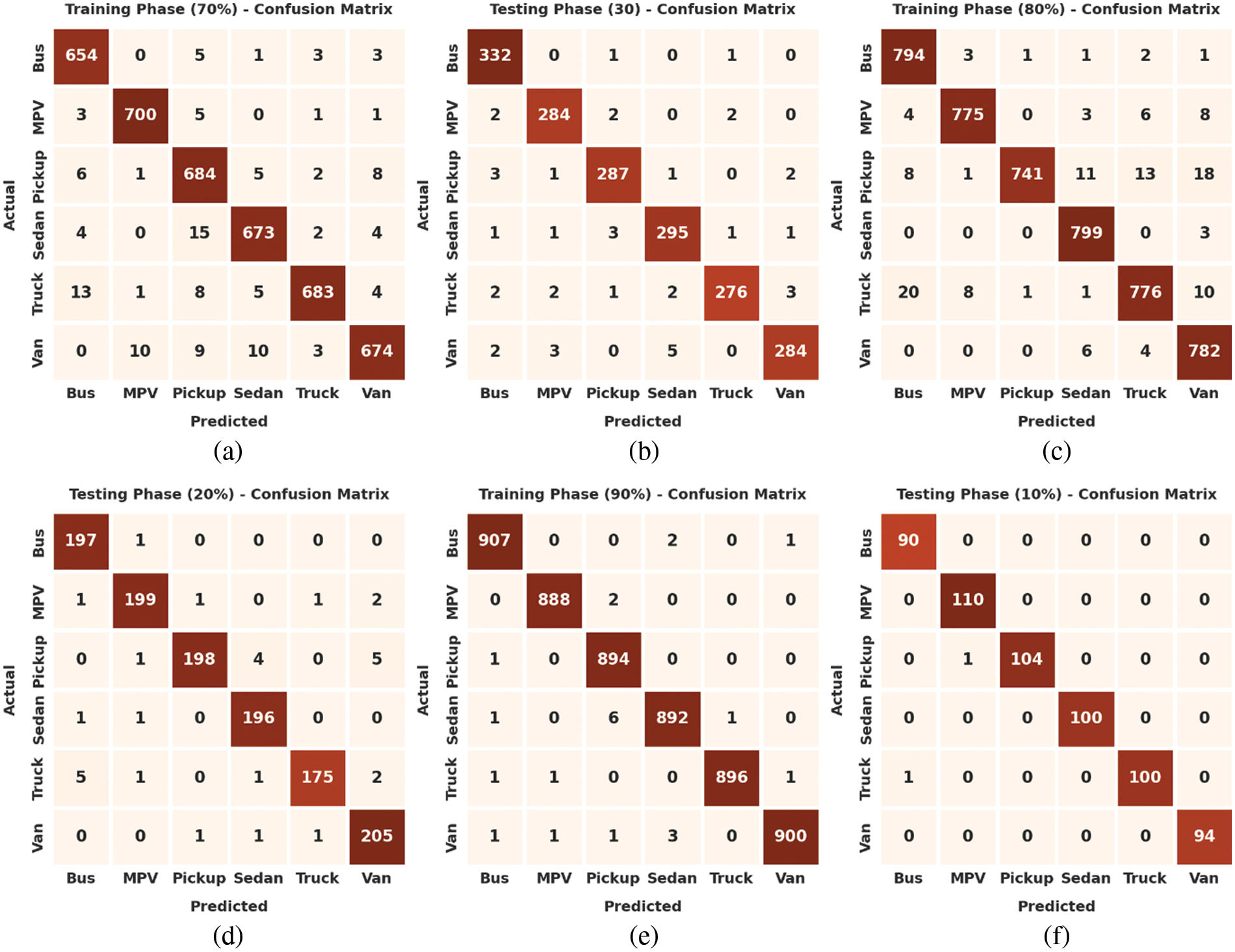
Figure 3: Confusion matrices of LSADTL-VCITS technique (a) 70% of TR data, (b) 30% of TS data, (c) 80% of TR data, (d) 20% of TS data, (e) 90% of TR data, and (f) 10% of TS data

Table 2 offers a detailed view on vehicle classification results accomplished by the proposed LSADTL-VCITS model under distinct aspects. Fig. 4 shows the comprehensive vehicle classification performance accomplished by the proposed LSADTL-VCITS model on 70% of TR data. The figure indicates that the proposed LSADTL-VCITS model achieved the maximum performance under all classes. For sample, LSADTL-VCITS model recognized the bus images with an accuy of 99.10%, precn of 96.18%, recal of 98.20%, and an Fscore of 97.18% respectively.

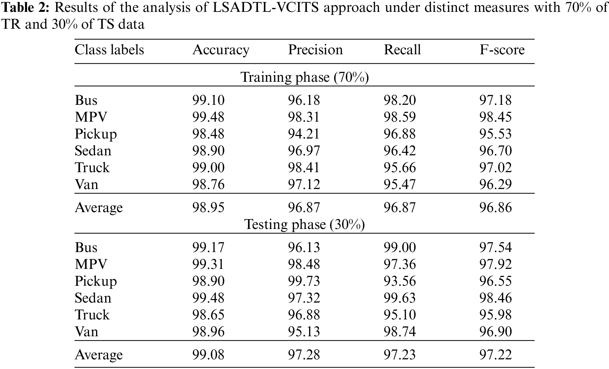
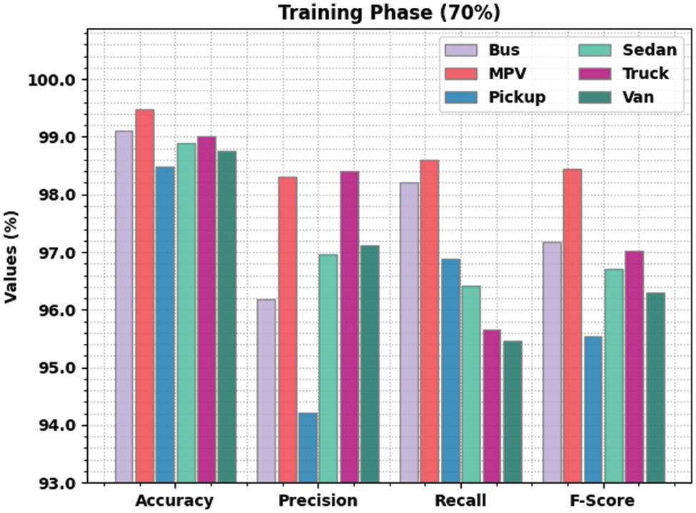
Figure 4: Results of the analysis of LSADTL-VCITS approach under 70% of TR data

The proposed LSADTL-VCITS system recognized the sedan images with an accuy of 98.90%, precn of 96.97%, recal of 96.42%, and an Fscore of 96.70% correspondingly. Moreover, LSADTL-VCITS algorithm recognized the van images with an accuy of 98.76%, precn of 97.12%, recal of 95.47%, and an Fscore of 96.29% correspondingly.

Fig. 5 shows the comprehensive vehicle classification performance achieved by the proposed LSADTL-VCITS approach on 30% of TS data. The figure exposes that the proposed LSADTL-VCITS algorithm achieved the maximal performance under all the classes. For sample, LSADTL-VCITS model recognized the bus images with an accuy of 99.17%, precn of 96.13%, recal of 99%, and an Fscore of 97.54% correspondingly. Similarly, LSADTL-VCITS model recognized the sedan images with an accuy of 99.48%, precn of 97.32%, recal of 99.63%, and an Fscore of 98.46% respectively. Moreover, the proposed LSADTL-VCITS method recognized the van images with an accuy of 98.96%, precn of 95.13%, recal of 98.74%, and an Fscore of 96.90% correspondingly.

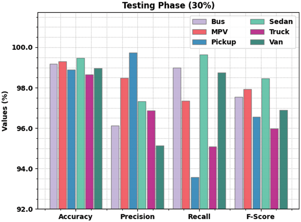
Figure 5: Results of the analysis of LSADTL-VCITS approach with 30% of TS data

Table 3 provides a detailed view on the vehicle classification outcome attained by the proposed LSADTL-VCITS system under distinct aspects. Fig. 6 shows the comprehensive vehicle classification performance achieved by the proposed LSADTL-VCITS model on 80% of TR data. The figure infers that the proposed LSADTL-VCITS model achieved the maximum performance under all the classes. For instance, LSADTL-VCITS model recognized the bus images with an accuy of 99.20%, precn of 97.48%, recal of 97.80%, and an Fscore of 97.64% correspondingly. Followed by, LSADTL-VCITS model recognized the sedan images with an accuy of 99.33%, precn of 98.87%, recal of 97.22%, and an Fscore of 97.93% correspondingly. Furthermore, LSADTL-VCITS methodology recognized the van images with an accuy of 99.26%, precn of 98.22%, recal of 97.35%, and an Fscore of 97.78% respectively.

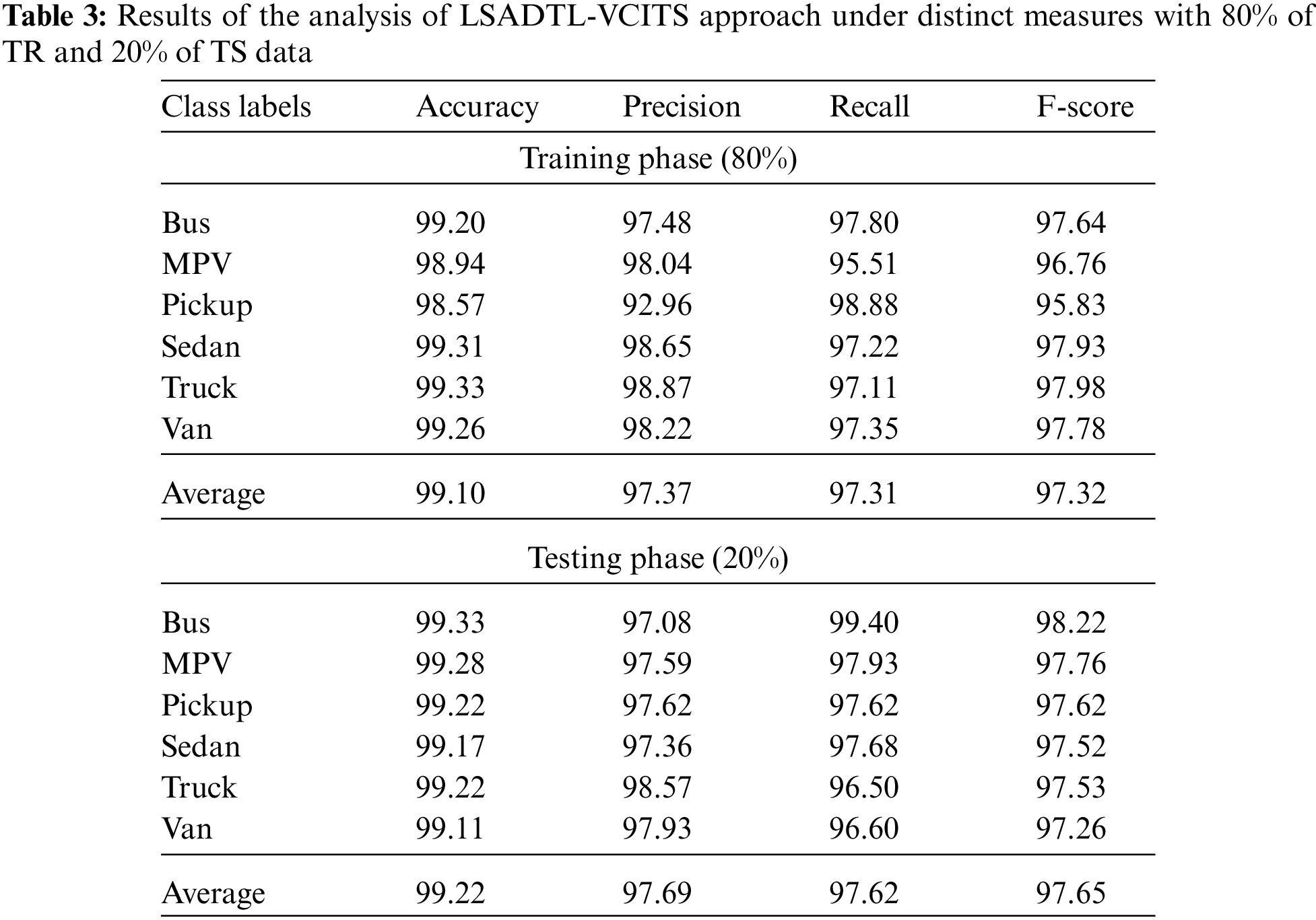
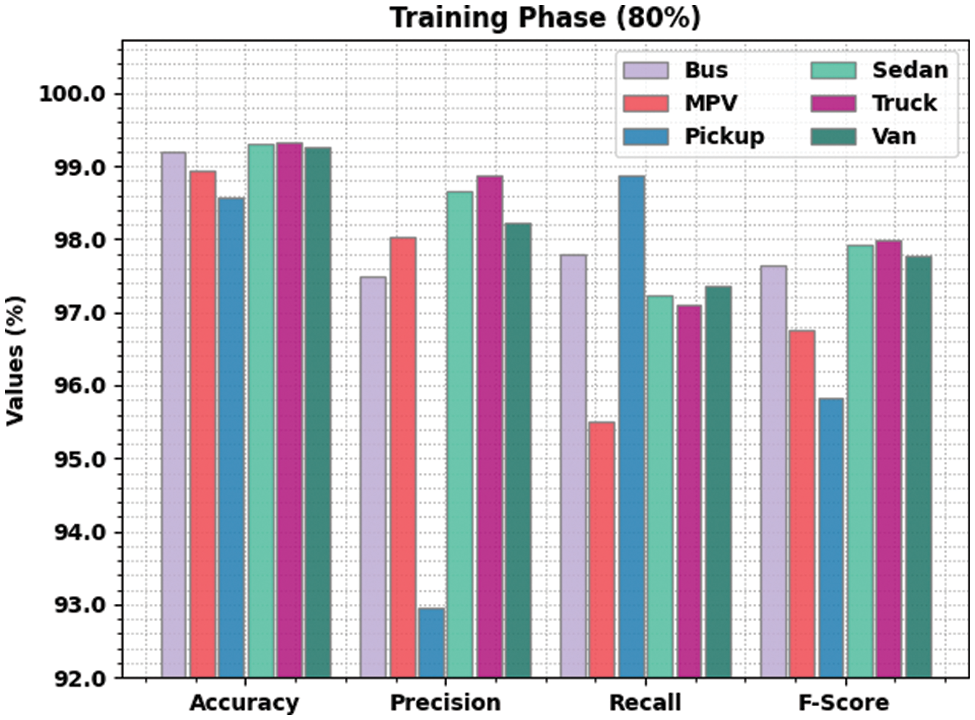
Figure 6: Results of the analysis of LSADTL-VCITS approach under 80% of TR data

Fig. 7 illustrates the comprehensive vehicle classification performance achieved by the proposed LSADTL-VCITS model on 20% of TS data. The figure reveals that the proposed LSADTL-VCITS approach attained the maximum performance under all the classes. For sample, the proposed LSADTL-VCITS technique recognized the bus images with an accuy of 99.33%, precn of 97.08%, recal of 99.40%, and an Fscore of 98.22% respectively. Likewise, LSADTL-VCITS system recognized the sedan images with an accuy of 99.17%, precn of 97.36%, recal of 97.68%, and an Fscore of 97.52% correspondingly. Additionally, the proposed LSADTL-VCITS methodology recognized the van images with an accuy of 99.11%, precn of 97.93%, recal of 96.60%, and an Fscore of 97.26% correspondingly.

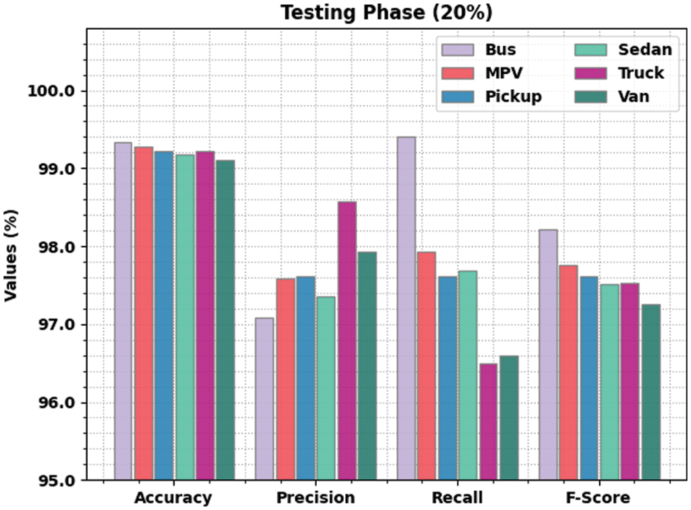
Figure 7: Results of the analysis of LSADTL-VCITS approach under 20% of TS data

Table 4 shows the detailed vehicle classification result yielded by the proposed LSADTL-VCITS methodology under different aspects. Fig. 8 depicts the comprehensive vehicle classification performance produced by the proposed LSADTL-VCITS model on 90% of TR data. The figure indicates that the proposed LSADTL-VCITS methodology reached the maximal performance under all the classes. For instance, the proposed LSADTL-VCITS system recognized the bus images with an accuy of 99.87%, precn of 99.56%, recal of 99.67%, and an Fscore of 99.62% respectively. Along with that, the proposed LSADTL-VCITS model recognized the sedan images with an accuy of 99.76%, precn of 99.44%, recal of 99.11%, and an Fscore of 99.28% respectively. Eventually, LSADTL-VCITS approach recognized the van images with an accuy of 99.85%, precn of 99.78%, recal of 99.34%, and an Fscore of 99.56% respectively.

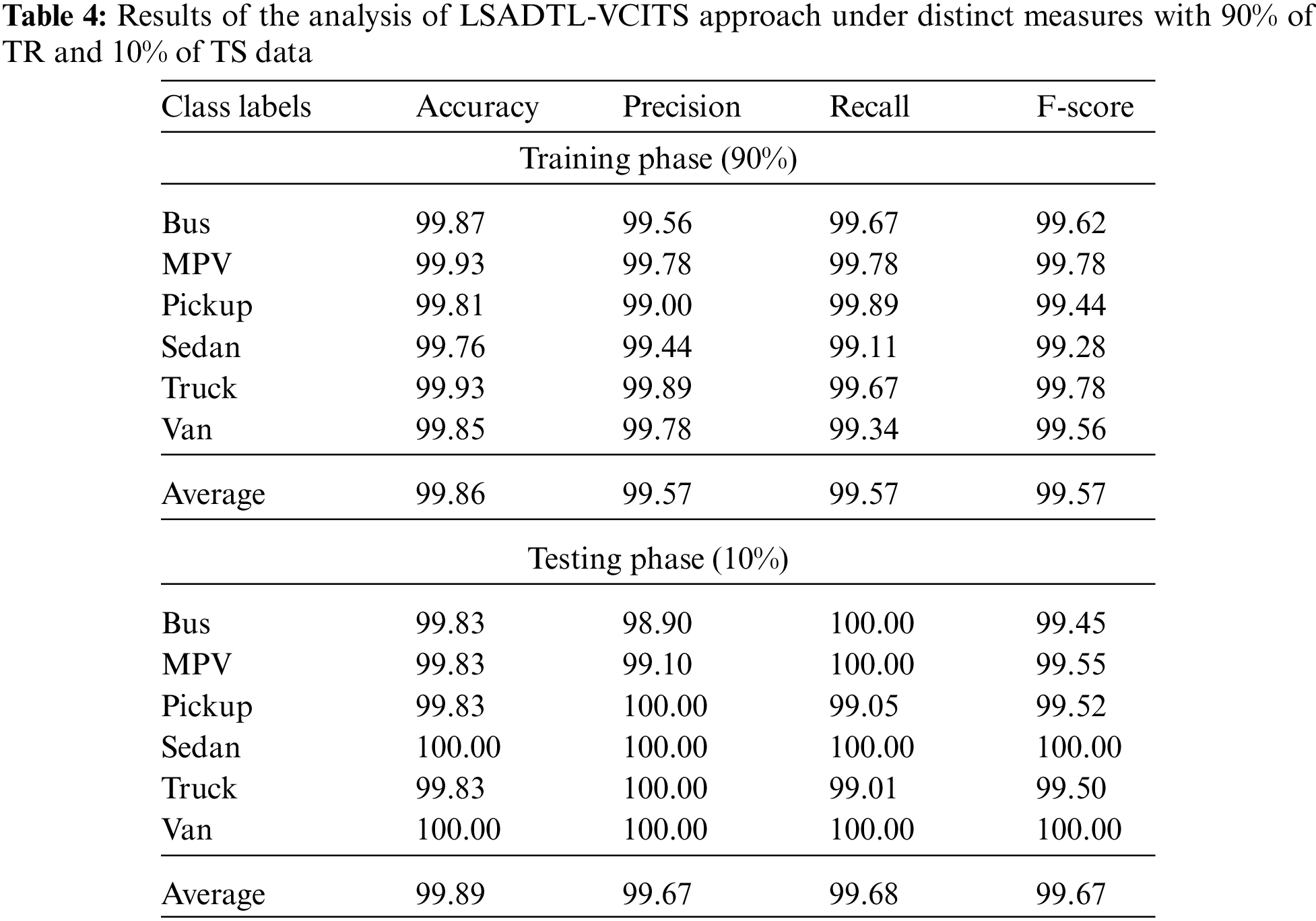
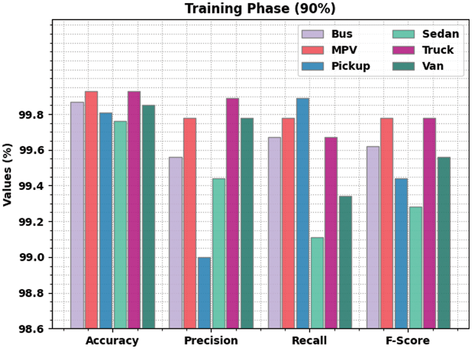
Figure 8: Results of the analysis of LSADTL-VCITS approach under 90% of TR data

Fig. 9 demonstrates the comprehensive vehicle classification performance attained by the proposed LSADTL-VCITS approach on 10% of TS data. The figure reveals that the proposed LSADTL-VCITS algorithm reached high performance under all the classes. For instance, LSADTL-VCITS model recognized the bus images with an accuy of 99.83%, precn of 98.90%, recal of 100%, and an Fscore of 99.45% correspondingly. Besides, the proposed LSADTL-VCITS approach recognized the sedan images with an accuy of 100%, precn of 100%, recal of 100%, and an Fscore of 100% correspondingly. Furthermore, the proposed LSADTL-VCITS method recognized the van images with an accuy of 100%, precn of 100%, recal of 100%, and an Fscore of 100% correspondingly.

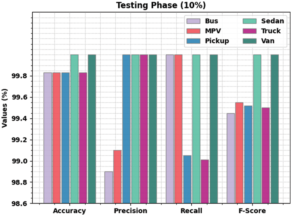
Figure 9: Results of the analysis of LSADTL-VCITS approach under 10% of TS data

Fig. 10 portrays the brief comparative accuracy analysis results accomplished by the proposed LSADTL-VCITS approach and other recent methodologies [11]. The results imply that the proposed LSADTL-VCITS model attained superior performance under all the classes. For instance, in bus class, LSADTL-VCITS model offered a high accuracy of 95.83%, whereas the CCLSTSV-CNN, CNN-Fusion, ensemble, Deep CNN, and CNN-AICITS models reported the least accuracy values such as 95.83%, 92.45%, 87.50%, 90.76%, and 99.55% respectively. In addition, in MPV class, the proposed LSADTL-VCITS technique obtained a superior accuracy of 99.83%, whereas CCLSTSV-CNN, CNN-Fusion, ensemble, Deep CNN, and CNN-AICITS approaches reported the least accuracy values such as 94.07%, 95.72%, 91.02%, 91.23%, and 99.53% correspondingly. Also, under Truck class, the proposed LSADTL-VCITS algorithm achieved an increased accuracy of 99.83%, whereas CCLSTSV-CNN, CNN-Fusion, ensemble, Deep CNN, and CNN-AICITS techniques reported minimal accuracy values such as 95.38%, 93.28%, 89.19%, 94.67%, and 99.57% correspondingly. At the same time, under Van class, the proposed LSADTL-VCITS approach achieved the highest accuracy of 100%, whereas CCLSTSV-CNN, CNN-Fusion, ensemble, Deep CNN, and CNN-AICITS methodologies reported the least accuracy values such as 92.79%, 91.94%, 88.85%, 89.90%, and 99.58% correspondingly.

Figure 10: Comparative analysis results of LSADTL-VCITS algorithm and other existing approaches

Finally, average accuracy analysis was conducted between LSADTL-VCITS model and other recent models and the results are shown in Fig. 11. The figure implies that ensemble model produced the least average accuracy of 88.63%. Simultaneously, deep CNN approach reached somewhat average accuracy of 92.90% whereas VCLSTSV-CNN and CNN-Fusion models reached reasonably closer average accuracy values such as 94.81% and 94.91% respectively. Though CNN-AICITS model reached a reasonable average accuracy of 99.58%, the proposed LSADTL-VCITS model achieved the maximum average accuracy of 99.89%. Based on these results and discussion, it is evident that the proposed LSADTL-VCITS model achieved effectual vehicle type classification performance in ITS environment.

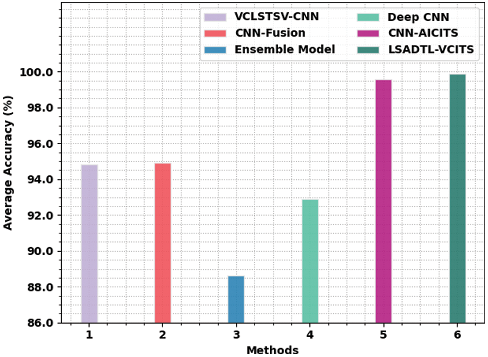
Figure 11: Average accuracy analysis results of LSADTL-VCITS algorithm and other existing approaches

5  Conclusion

In this study, a novel LSADTL-VCITS approach has been designed and developed for vehicle classification in the ITS environment. The presented LSADTL-VCITS approach encompasses two major stages namely vehicle detection and vehicle classification. At the initial stage, the YOLO-v5 model has been applied for vehicle recognition process. Next, in the second stage, LSA is utilized with MLP model for the classification of vehicles under distinct classes. The performance of the proposed LSADTL-VCITS approach is validated utilizing benchmark dataset and the outcomes were inspected under several measures. The experimental outcomes highlighted the better performance of the LSADTL-VCITS model over recent approaches. Thus, the presented LSADTL-VCITS model can be utilized as a proficient tool for vehicle classification in the ITS environment. In future, hybrid DL methods can be utilized to enhance the classification performance in the ITS environment.

Funding Statement: The authors received no specific funding for this study.

Conflicts of Interest: The authors declare that he has no conflicts of interest to report regarding the present study.

References

1. J. T. Lee and Y. Chung, “Deep learning-based vehicle classification using an ensemble of local expert and global networks,” in 2017 IEEE Conf. on Computer Vision and Pattern Recognition Workshops (CVPRW), Honolulu, HI, USA, pp. 920–925, 2017. [Google Scholar]
2. C. Chen, B. Liu, S. Wan, P. Qiao and Q. Pei, “An edge traffic flow detection scheme based on deep learning in an intelligent transportation system,” IEEE Transactions on Intelligent Transportation Systems, vol. 22, no. 3, pp. 1840–1852, 2021. [Google Scholar]
3. H. Nguyen, L. Kieu, T. Wen and C. Cai, “Deep learning methods in transportation domain: A review,” IET Intelligent Transport Systems, vol. 12, no. 9, pp. 998–1004, 2018. [Google Scholar]
4. I. Abunadi, M. M. Althobaiti, F. N. Al-Wesabi, A. M. Hilal, M. Medani et al., “Federated learning with blockchain assisted image classification for clustered UAV networks,” Computers, Materials & Continua, vol. 72, no. 1, pp. 1195–1212, 2022. [Google Scholar]
5. A. Gholamhosseinian and J. Seitz, “Vehicle classification in intelligent transport systems: An overview, methods and software perspective,” IEEE Open Journal of Intelligent Transportation Systems, vol. 2, pp. 173–194, 2021. [Google Scholar]
6. M. Al Duhayyim, H. M. Alshahrani, F. N. Al-Wesabi, M. Abdullah Al-Hagery, A. Mustafa Hilal et al., “Intelligent machine learning based EEG signal classification model,” Computers, Materials & Continua, vol. 71, no. 1, pp. 1821–1835, 2022. [Google Scholar]
7. A. M. Hilal, H. Alsolai, F. N. Al-Wesabi, M. K. Nour, A. Motwakel et al., “Fuzzy cognitive maps with bird swarm intelligence optimization-based remote sensing image classification,” Computational Intelligence and Neuroscience, vol. 2022, no. 4, pp. 1–12, 2022. [Google Scholar]
8. S. Yu, Y. Wu, W. Li, Z. Song and W. Zeng, “A model for fine-grained vehicle classification based on deep learning,” Neurocomputing, vol. 257, no. 2, pp. 97–103, 2017. [Google Scholar]
9. W. Maungmai and C. Nuthong, “Vehicle classification with deep learning,” in 2019 IEEE 4th Int. Conf. on Computer and Communication Systems (ICCCS), Singapore, pp. 294–298, 2019. [Google Scholar]
10. P. Wang, W. Hao and Y. Jin, “Fine-grained traffic flow prediction of various vehicle types via fusion of multisource data and deep learning approaches,” IEEE Transactions on Intelligent Transportation Systems, vol. 22, no. 11, pp. 6921–6930, 2021. [Google Scholar]
11. S. Srivastava, S. Narayan and S. Mittal, “A survey of deep learning techniques for vehicle detection from UAV images,” Journal of Systems Architecture, vol. 117, no. 11, pp. 102152, 2021. [Google Scholar]
12. N. Kavitha and D. N. Chandrappa, “Optimized YOLOv2 based vehicle classification and tracking for intelligent transportation system,” Results in Control and Optimization, vol. 2, no. 3, pp. 100008, 2021. [Google Scholar]
13. Z. Lv, S. Zhang and W. Xiu, “Solving the security problem of intelligent transportation system with deep learning,” IEEE Transactions on Intelligent Transportation Systems, vol. 22, no. 7, pp. 4281–4290, 2021. [Google Scholar]
14. M. A. Butt, A. M. Khattak, S. Shafique, B. Hayat, S. Abid et al., “Convolutional neural network based vehicle classification in adverse illuminous conditions for intelligent transportation systems,” Complexity, vol. 2021, no. 1, pp. 1–11, 2021. [Google Scholar]
15. K. Yu, L. Lin, M. Alazab, L. Tan and B. Gu, “Deep learning-based traffic safety solution for a mixture of autonomous and manual vehicles in a 5G-enabled intelligent transportation system,” IEEE Transactions on Intelligent Transportation Systems, vol. 22, no. 7, pp. 4337–4347, 2021. [Google Scholar]
16. L. Qiu, D. Zhang, Y. Tian and N. Al-Nabhan, “Deep learning-based algorithm for vehicle detection in intelligent transportation systems,” The Journal of Supercomputing, vol. 77, no. 10, pp. 11083–11098, 2021. [Google Scholar]
17. J. Ashraf, A. D. Bakhshi, N. Moustafa, H. Khurshid, A. Javed et al., “Novel deep learning-enabled LSTM autoencoder architecture for discovering anomalous events from intelligent transportation systems,” IEEE Transactions on Intelligent Transportation Systems, vol. 22, no. 7, pp. 4507–4518, 2021. [Google Scholar]
18. C. C. Tsai, C. K. Tseng, H. C. Tang and J. I. Guo, “Vehicle detection and classification based on deep neural network for intelligent transportation applications,” in 2018 Asia-Pacific Signal and Information Processing Association Annual Summit and Conf. (APSIPA ASC), Honolulu, HI, USA, pp. 1605–1608, 2018. [Google Scholar]
19. X. Wang, J. Liu, T. Qiu, C. Mu, C. Chen et al., “A real-time collision prediction mechanism with deep learning for intelligent transportation system,” IEEE Transactions on Vehicular Technology, vol. 69, no. 9, pp. 9497–9508, 2020. [Google Scholar]
20. Q. Xu, Z. Zhu, H. Ge, Z. Zhang and X. Zang, “Effective face detector based on YOLOv5 and superresolution reconstruction,” Computational and Mathematical Methods in Medicine, vol. 2021, no. 4, pp. 1–9, 2021. [Google Scholar]
21. C. Xiang, L. Zhang, Y. Tang, W. Zou and C. Xu, “MS-CapsNet: A novel multi-scale capsule network,” IEEE Signal Processing Letters, vol. 25, no. 12, pp. 1850–1854, 2018. [Google Scholar]
22. M. Ragab, A. Albukhari, J. Alyami and R. F. Mansour, “Ensemble deep-learning-enabled clinical decision support system for breast cancer diagnosis and classification on ultrasound images,” Biology, vol. 11, no. 3, pp. 439, 2022. [Google Scholar]
23. A. S. Hassan, Y. Sun and Z. Wang, “Optimization techniques applied for optimal planning and integration of renewable energy sources based on distributed generation: Recent trends,” Cogent Engineering, vol. 7, no. 1, pp. 1766394, 2020. [Google Scholar]
24. https://www.v7labs.com/open-datasets/veri-dataset. [Google Scholar]
Cite This Article
Copyright © 2023 The Author(s). Published by Tech Science Press.
This work is licensed under a Creative Commons Attribution 4.0 International License , which permits unrestricted use, distribution, and reproduction in any medium, provided the original work is properly cited.
Downloads
Citation Tools