MI-STEG: A Medical Image Steganalysis Framework Based on Ensemble Deep Learning

1  Introduction

Image steganography involves embedding a hidden message into a cover image, with the resulting stego image transmitted to the receiver through a communication channel without third parties noticing [1]. Although the first steganography techniques were mainly aimed at providing imperceptibility, recent studies focus on developing models that will increase imperceptibility, capacity, and robustness against steganalysis attacks [2,3]. Image steganalysis aims to detect the hidden data in a cover image by performing passive or active attacks [4,5]. A passive attack is used to determine the evidence of the hidden data in a cover image, while an active attack decrypts the steganography scheme. In this context, the clairvoyant scenario and the cover-stego mismatch scenario are implemented in steganalysis studies. In the case of the clairvoyant scenario, the steganalyst is assumed to know the embedding algorithm, the payload of the hidden data, the image sizes, and the image database employed. In addition, it is assumed that the same stego key is used in all images [6]. In the mismatch scenario, on the other hand, there is no information at hand about the steganography scheme or the payload of the hidden data to help decide whether an image is a cover or a stego.

Image steganalysis is a binary classification problem. Traditional steganalysis techniques solve this problem using machine learning (ML) or statistical approaches. Earlier steganalysis studies proposed statistical approaches to detect the hidden data embedded with the least significant bit (LSB) method. Essentially there are three techniques to achieve this: chi-square, regular singular (RS), and sample pair analysis (SPA). In the chi-square technique, the image is segmented, and the presence of the message is traced based on the statistical change in the chi-square coefficients of each segmented block. RS steganalysis analyzes the images using spatial correlation. To detect the stego-signal, the pixels in the image are divided into three groups with reference to their neighborhood: regular, singular, and unusable [7]. Finally, in the SPA technique, images (or blocks) are evaluated in pairs using high-order statistical calculations to determine the length of messages embedded with LSB [8]. When RS and SPA procedures are not optimized properly, they cannot be successful in the steganalysis of the LSB technique, which entails random data insertion into a cover image [9].

In recent years, ML techniques have been increasingly applied in image steganalysis. ML is comprised of two stages: feature extraction and classification. Feature analysis seeks and identifies the special features related to the distortion caused by the steganography method. Features are obtained by complex analyzes such as subtractive pixel adjacency matrix (SPAM), spatial-domain rich model (SRM), and max spatial-domain rich model (maxSRM), which are high-dimensional [5,7,10]. The second step involves classification using a decision tree, k-nearest neighbor (kNN), support vector machines (SVM) [9], artificial neural networks (ANN) [9,11–13], or fisher linear discriminants (FLD) [7] with an ensemble classifier and random forest. The performance of the ML classifiers is highly dependent on the selected features. Yet, the features that are more effective remain unknown in classification [5].

Deep learning (DL) architectures have been used recently in image steganalysis because they perform feature analysis within convolutional blocks. In studies employing such architectures, data at different bpp (bit per pixel) ratios were hidden into the images on the break our steganographic system base (BOSSBase) dataset by spatial domain embedding methods such as highly undetectable stego (HUGO), wavelet obtained weights (WOW), and spatial version of the universal wavelet relative distortion (S-UNIWARD).

2  Related Works

Tan et al. [14] proposed the first convolutional neural network (CNN) for image steganalysis in 2014, obtaining a 48% detection error for the HUGO approach with a 0.4 bpp payload. Qian et al. [15] used a 5 × 5 high-pass filter (HPF) in the input layer of the CNN. HPF strengthened the low stego-noise signal caused by data hiding in the cover image and ensured that this information was not forgotten in the deep network. Gaussian activation function after convolution layers followed by average pooling was also introduced in the feature extraction layers of CNN. However, these achieved lower accuracy than that of the SRM technique. In another study [16], CNN architectures were first trained to detect different payload rates of a data hiding method. The network weights trained using cover images and stego images with high bpp rates were transferred downstream to the DL architectures for the same embedding method with lower bpp rates. The obtained results showed that transfer learning improves network performance as expected.

To capture the stego-noise signal in the feature layers of the DL architecture, subsequent studies investigated the effects of specific layers, kernel sizes, and activation function types on steganalysis performance. The model proposed by Xu et al. [17] calculated the absolute values of the features in the first convolution layer and then applied the batch normalization (BN) and tangent hyperbolic (tanH) activation functions. In the deeper convolution layers, a 1 × 1 kernel size was used to obtain the stego-signal. The performance results obtained for the high-pass, low-pass, and low-pass (HILL) and S-UNIWARD techniques competed with those of the SRM classifier. Ye et al. [18] adapted the HPFs set used to calculate residual maps in the SRM classifier technique to the input layer of the CNN model. They used the truncated linear unit (TLU) activation function to capture the stego signal in the deep feature layers. The detection error rates of the model were relatively high compared to those achieved with the SRM classifier technique. These studies [17,18] show that using specific building blocks to learn the features of the stego-signal in the initial convolution layers improves the performance of the deepening network architecture. Therefore, in later studies, it was possible to develop deeper DL architectures using big data.

In the DL architecture [6], augmented BOSSBase and LIRMMBase datasets subjected to cropping were analyzed for clairvoyant and cover-source mismatch scenarios. Qian et al. [15,16] presented the images after HPF preprocessing to the CNN model and then used the rectified linear unit (ReLU) activation function in the feature layers. As stated in [19], pooling layers were not used because the down-sampling process has a denoising effect on the feature maps. In the study, the model’s classification accuracy increased by 8% when the pooling layer was omitted. However, this modification resulted in a higher number of trainable network parameters.

The increasing number of layers in deep models causes catastrophic forgetting. The proposed residual neural network (ResNet) model was also used in image steganalysis to overcome this problem. In this model, which differs from the typical CNN architecture essentially with the cascade layer structure, residual blocks are used, and the inputs of these blocks are directly connected to their outputs in a second way. The literature analyzed the hypothesis that residual learning can distinguish a low stego signal from the image content. Wu et al. [20] used bottleneck and non-bottleneck building blocks to provide learning and increase size after applying HPF to images. In the study, the detection error decreased as the number of convolution layers increased. In another DL architecture [21], RestegNet, connection-based sharpening and smoothing blocks enabled the stego signal detection and the feature maps’ subsampling to decompose the stego signal, respectively. Boroumand et al. [22] designed a residual-learning model with four different feature extraction blocks for noise detection. The first two layers lacked residual connections and pooling, whereas the subsequent seven layers contained residual connections without pooling. The four layers to follow applied residual connections and average pooling. The final layer of features consisted of a global average pooling layer. Even though the model was primarily designed for joint photographic experts group (JPEG) steganalysis, the spatial steganalysis performance levels of the S-UNIWARD, HILL, and WOW methods were high. The Zhu-NET architecture proposed by Zhang et al. [23] used trainable filters with 3 × 3 kernels instead of fixed filters in the preprocessing layer. Feature layers of the model with single residual links had separable convolutions and spatial pyramid pooling instead of global average pooling in the last layer. Reinel et al. [24] used depthwise and separable convolutional layers and two residual connections in their proposed GBRAS-Net model. Another study [25] proposed the SFRNET model with re-parameterization Visual Geometry Group architecture (RepVGG) and squeeze-and-excitation blocks in feature extraction layers. In summary, extracting features without losing low stego-noise is challenging, and using blocks with residual links improves performance.

The proposed CNN models for the steganalysis of spatial or JPEG embedding techniques with 0.1 and 0.2 bpp payloads did not achieve a high level of performance. To overcome this problem, transfer learning has been utilized. Ozcan et al. [26] sequentially down-transferred the weights of the ResNet50 networks trained with cover and stego images containing hidden data with different payloads for the HUGO and WOW methods to find that transfer learning (TFL) increased the performance of stego-signal detection compared to conventional training. Similarly, pre-trained deep models were used for spatial and JPEG image steganalysis to show that TFL improved performance [27]. Another way to improve detection performance in image steganalysis is to ensemble the classifiers. Xu et al. [28] achieved better performance than traditional SVM in steganalysis of three different JPEG hiding techniques with the proposed ensemble model. In the MixNet model proposed by Amrutha et al. [29], the features obtained separately from six distinct CNN architectures were concatenated. Then these features are classified with the SVM classifier. The ensemble CNN model produced high detection accuracy for HUGO, S-UNIWARD, and WOW methods.

The aim of the present study is to perform medical image steganalysis with pre-trained DL models, based on the existing literature on image steganalysis. For this reason, an original dataset containing brain magnetic resonance imaging (MRI) images were prepared for medical image steganalysis. For the cover-source mismatch scenario, random data in the range of 1.0–0.1 bpp payloads were hidden into the cover images using the HUGO, minimizing the power of optimal detector (MIPOD), and S-UNIWARD embedding methods. In the deep DL architecture, the low stego-signal was amplified by first applying HPF to the images. The architectures of medical image steganalysis networks with payload were transferred separately from the dense convolutional network (DenseNet), ResNet, and Inception models. The steganalysis outputs of these networks were determined by assembling TFL models separately for each spatial embedding method with different payload ratios. The actual performances of the networks were compared against the predicted levels using metrics such as detection error, precision, recall, accuracy, and F1-score.

The study set out to achieve the following as contributions to the literature:

(1)   Developing an ensemble-based DL framework for medical image steganalysis for the first time in literature.

(2)   Detecting whether a medical image contains hidden data that can be used for malicious purposes in open networks.

(3)   Adaptation of difficult-to-detect image steganalysis techniques to medical image steganalysis.

(4)   Determining the role of pre-trained DL models to detect medical image steganalysis.

(5)   Contributing to developing new medical image steganography methods against the DL-based steganalysis model.

3  Medical Image Steganalysis Framework

The deep ensemble model proposed for medical image steganalysis comprises three stages: pre-processing, classification, and assembling the TFL-based CNN models, as shown in Fig. 1.

Figure 1: The flowchart of the medical image steganalysis framework

In the study, datasets containing ten different cover-stego image pairs with payloads in the 0.1–1.0 bpp range were prepared for each HUGO, MIPOD, and S-UNIWARD embedding technique. In addition, a base-training dataset was created by hiding 1.0 bpp payload data on cover medical images using the LSB steganography technique. The pre-processing stage involved amplifying the low-stego signal by applying the HPF to distinguish it from the image content, as detailed below [15–18,30]. Secondly, TFL-based CNN models were trained separately using the prepared datasets to detect ten different payload rates carried by three distinct embedding techniques. In the study, feature layers of CNN architectures were transferred from eleven TFL-based models, including three DenseNet models (DenseNet121, DenseNet169, and DenseNet201) [31], six ResNet models (ResNet50, ResNet101, ResNet152, ResNet50V2, ResNet101V2, and ResNet152V2) [32], and two Inception models (InceptionV3, and InceptionResNetV2) [33].

The training strategy for these pre-trained CNN models is as follows:

(1)   Each model was trained separately using the LSB base training set.

(2)   Next, the CNN models to classify the 1.0 bpp ratio of the three embedding methods were trained by initializing with the weights of these pre-trained models.

(3)   For each hiding method, the model weights are sequentially transferred to CNN models that will classify different payloads starting from 1.0 bpp down to 0.1 bpp.

Finally, the classification performance of each embedding technique with a different payload was determined by assembling the results of the eleven models using the test dataset. The obtained outputs of all models and the real outputs were compared using the accuracy, detection error (DE), recall, precision, correlation coefficient (R), and F1-score performance metrics.

3.1 Medical Image Dataset

In this study, axial, coronal, and sagittal slices of T1, T2, and fluid-attenuated inversion recovery (FLAIR) weighted MRI images, which are in two different data sets, were combined for medical image steganalysis. The first dataset contains images of 15 epilepsy patients and 15 healthy individuals obtained from Gazi University Faculty of Medicine, Department of Neurology [1]. The second dataset contains brain images of 30 patients with focal epilepsy obtained from the Department of Neurology and Radiology at Cumhuriyet University [34]. The dataset combining 5961 images was divided into training and validation sets, which contained 90% and 10% of all images, respectively. As the study adopted a cover-stego mismatch scenario, a different dataset containing 3064 T1-weighted brain MR images was used as a testing set [35]. The “.dcm” images of different sizes in the training and test set were resized to 224 × 224.

S-UNIWARD, HUGO, and MIPOD techniques (http://dde.binghamton.edu/download/) were used to prepare the stego images. These techniques cause low levels of distortion on the image and are difficult to statistical distribution steganalysis. Ten different datasets were created for each data hiding technique with payloads in the range 1.0 to 0.1 bpp. Fig. 2 shows cover and stego image pairs and the difference images obtained between them. Data hiding was found to cause 1-pixel increases or decreases in image sizes potentially. Therefore, as the amount of payload decreases, the distortion caused by the stego signal in the images decreases, as seen in Fig. 2.

Figure 2: Cover, stego, and difference images for 0.2, 0.4, and 1.0 bpp payloads, a) HUGO method, b) MIPOD method, c) S-UNIWARD method

3.2 Pre-Processing Module

The input information to be presented to the network is prepared in the pre-processing image layer. In this layer, filtering is performed using a fixed high-pass filter (KHPF) with a 5 × 5 kernel size, for the high-frequency stego-noise added to the cover image is a weak signal that is significantly affected by the image content. Because of the high-frequency filtering, the weak stego signal is amplified to distinguish it from the content, resulting in an image expressed as a residual image (IR), as given in Eq. (1) [15,16].

IR=KHPF∗Iinput

KHPF=112(−12−22−12−68−62−28−128−22−68−62−12−22−1)(1)

3.3 Transfer Learning Based Deep Learning Models

CNN is a DL method that automates feature extraction in a classification problem, unlike other machine learning (ML) techniques. While the filters used for feature extraction in ML are obtained manually or by optimization techniques, CNN learns its filters without any prior knowledge or human dependency. CNN comprises multiple building blocks such as convolutional layers, pooling layers, and fully connected layers (FCLs). Randomly initialized filter values in convolutional layers are updated by error back-propagation. The features of the input image are learned by preserving the relationships between the pixels. In the CNN, the feature value zi,j,kl at the (i, j) position of the kth feature map and the lth layer is calculated through Eq. (2) [36–39].

zi,j,k=lwklTxi,jl+bkl(2)

where wkl and bkl represent the weight vector and bias vector for the kth filter and lth layer, respectively. xi,jl represents the input at position (i, j) in the lth layer. The feature values (zi,j,kl) obtained by convolution in CNN are made nonlinear (a(zi,j,kl)) by means of an activation function such as sigmoid, tanh, or ReLU [36–39]. In the pooling layer, subsampling ((yi,j,k=lpool(a(.)) is performed to reduce the size of feature maps and the number of trainable parameters of the network.

After the last convolution or pooling layer of feature extraction layers in the CNN, FCLs are used to flatten the feature maps into a one-dimensional vector. Each neuron of the FCL multiplies its inputs by a weight vector and adds a bias vector. The net information is then processed by an activation function such as ReLU. The outputs of FCL are connected to all inputs of the subsequent fully connected layer [36–39].

The classification layer, which is the final layer, often uses the softmax function to calculate the probabilities of the network’s outputs. The learnable parameters of the CNN (θ={W,B}, W: weights, B: biases) are updated iteratively using an objective function that minimizes the difference between the actual and calculated outputs of the network, as shown in Eq. (3).

L=1N∑n=1Nl(θ;y(n),o(n))(3)

where y(n) and o(n) represent the nth real output and the predicted output of the CNN, respectively [39].

Deep networks designed to achieve high-performance values in medical steganalysis need to overcome two main challenges. The first of these is to extract features without losing low stego-noise information, and the second is the vanishing gradient problem. To overcome these problems, residual connections have been proposed [31,32]. In traditional CNN architecture, xℓ, which is the output of the lth layer, is the input of the following (ℓ+1)th layer. This transition between layers is expressed by the formula xℓ=Hℓ(xℓ−1). Nonlinear transformation Hℓ(⋅) includes convolution, pooling, BN, ReLU, etc. In the ResNet network, a transition link is added to nonlinear transformation (Hℓ(⋅)) with an identity function, which transfers the gradients between the layers, as illustrated in Eq. (4) and Fig. 3 [31,32].

xℓ=Hℓ(xℓ−1)+xℓ−1(4)

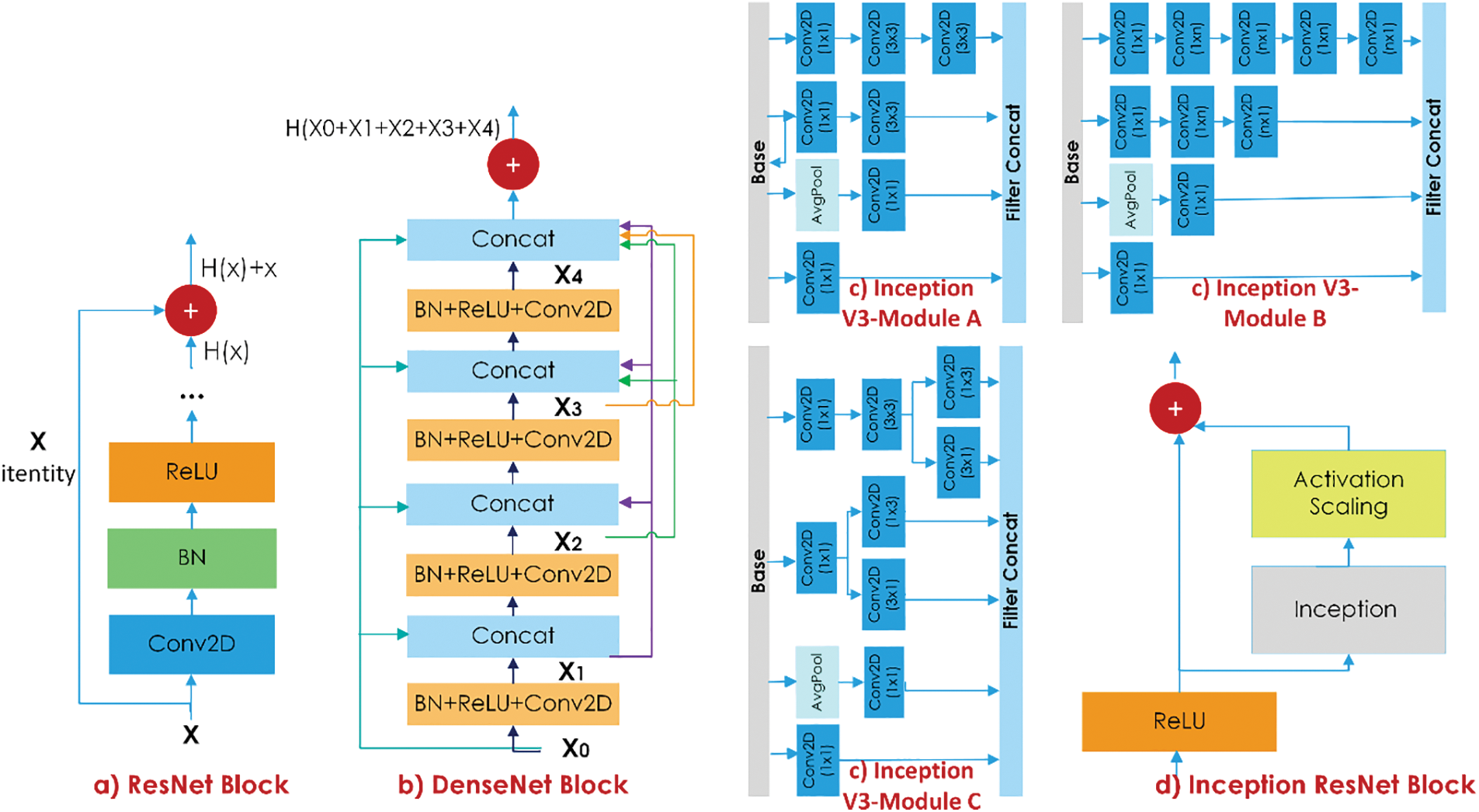
Figure 3: The representation of ResNet, DenseNet, Inception V3, and Inception ResNet blocks

Combining the identity function and the output of Hℓ(⋅) by summarizing each layer causes the information flow problem. In DenseNet architecture, each layer is directly connected with other subsequent layers to solve this problem [31]. The lth layer in the network with inputs x0,…,xℓ−1 receives the features of the previous layers, as shown in Eq. (5) and Fig. 3.

xℓ=Hℓ([x0,x1,…,xℓ−1])(5)

In deep networks, the vanishing gradient problem is accompanied by the computational cost issue as well. As a solution, inception modules, which enable parallel network extension, have been proposed [33]. In a basic inception module, convolution with 1 × 1, 3 × 3, and 5 × 5 filter kernels and maximum pooling are performed in parallel. Nonetheless, there is still a computational cost in this parallel expansion. The network’s size and convergence speed were proved by adding 1 × 1 convolution layers to the beginning of the inception modules [33]. In the Inception-ResNet model, a mix of inception modules and residual connections is used, as shown in Fig. 3.

In the MI-STEG model proposed in this study, ResNet, DenseNet, and Inception architectures were trained separately for three hiding techniques with each payload, and the results of the TFL-based models for each method were assembled using an average layer.

3.4 Experiment Setup

The proposed MI-STEG model was implemented using the Tensorflow-based Keras library in Python. Experiments were performed on a computer equipped with an NVIDIA Tesla K80 24 gigabyte (GB) graphics processing unit (GPU), an Intel Xeon ES-2680 V4 @ 2.40 gigahertz (GHz) central processing unit (CPU), and 128 GB random access memory (RAM). The trainable parameters of the CNNs were optimized with the stochastic gradient descent (SGD) optimization technique. The momentum, learning rate, and weight decay were respectively set to 0.99, 0.0001, and 0.00001. Dropout and Ridge regression (L2) regularization were implemented to prevent the overfitting problem in training CNNs. In addition, the weights of non-overfitting networks with the best validation accuracy were recorded, and CNN models were tested using these weights. The training epoch and batch size are 20 and 32, respectively. Five-fold cross-validation was used to repeat training for each CNN.

3.5 Evaluation Methods

In the study, MI-STEG’s performance in detecting hidden messages in medical images was measured using the specificity, accuracy, DE (1-accuracy), precision, recall, F1-score, and R values. The confusion matrix is used to evaluate the classification performance in the ML, and it calculates true positive (TP), false positive (FP), true negative (TN), and false negative (FN) values that indicate true positive, false positive, true negative, and false negative, respectively. Specificity indicates the ratio at which a classifier predicts true negative samples (Specificity=TN/(TN+FP)). The accuracy shows the percentage of the inputs predicted correctly (Accuracy=(TP+TN)/(TP+TN+FP+FN)).

Precision indicates how many medical images in stego class are correctly predicted, as illustrated in Eq. (6).

Precision=TP/(TP+FP)(6)

Recall shows the ratio of positives correctly categorized, as given in Eq. (7).

Recall=TP/(TP+FN)(7)

F1-score indicates the harmonic average of precision and recall values, as represented in Eq. (8).

F1=2Precision.RecallPrecision+Recall=2TP2TP+FP+FN(8)

R calculates the relationship between the real outputs (x) and predicted outputs (y) using Eq. (9).

R=∑(x−x¯)(y−y¯)∑(x−x¯)2∑(y−y¯)2(9)

where x¯ is the mean of real outputs and y¯ is the mean of predicted outputs.

4  Results and Discussion

This section presents the performance results from the three TFL-based models and the proposed MI-STEG model. The results were compared to previous DL-based image steganalysis studies in the literature.

4.1 Experiment Results

Table 1 shows the performance results of the DL models used in the study, detecting the HUGO technique with 0.2 and 0.4 bpp payloads. While all models are successful in detecting 0.4 bpp, it can be said that deeper DL networks are more successful in detecting 0.2 bpp payload. On the other hand, the MI-STEG model achieved the highest performance values in detecting both payloads.

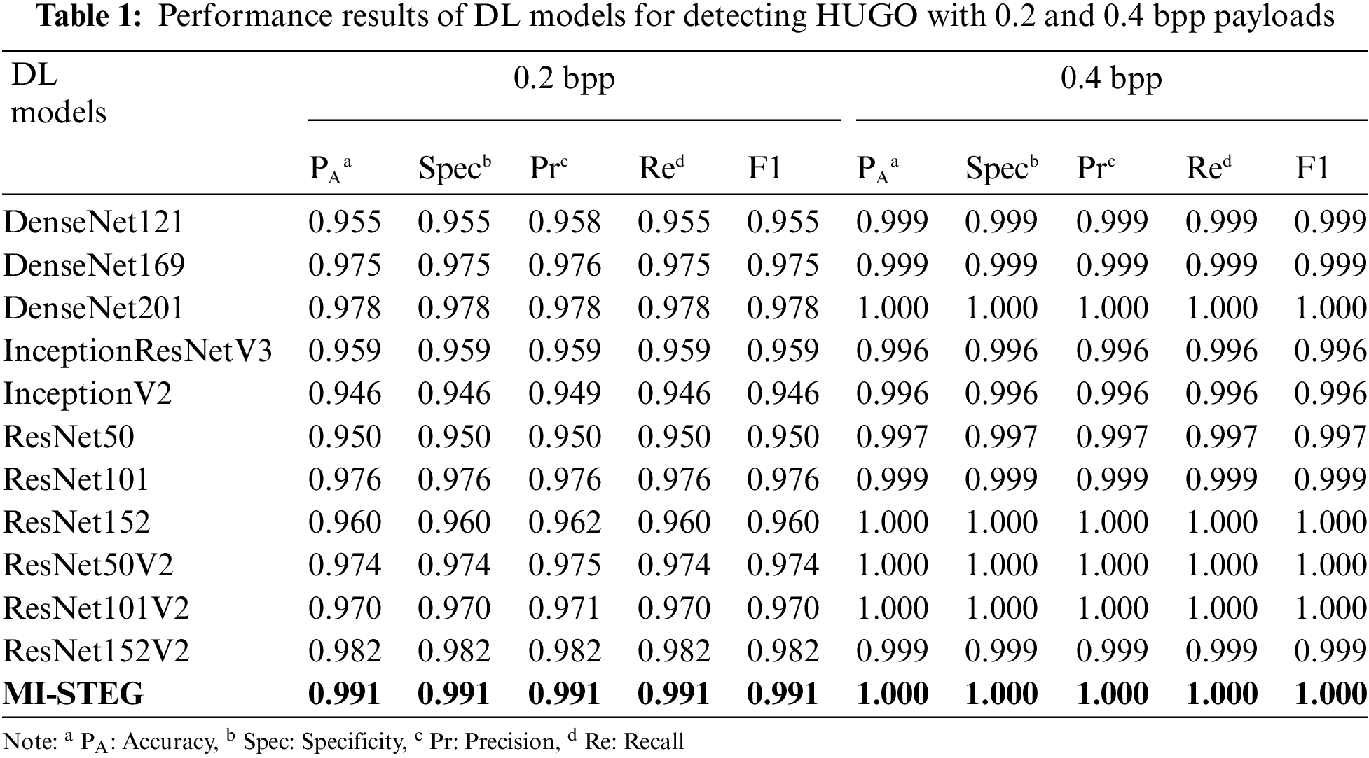
Fig. 4 shows the detection error and R values obtained by the DL models for detecting the HUGO method at different loads. The detection errors of the models for 0.1 and 0.2 bpp range from 0.106 to 0.193 and 0.009 to 0.054, respectively. The R values of the CNNs for 0.1 and 0.2 bpp range from 0.616 to 0.791 and 0.895 to 0.982, respectively. As expected, as the payload increased, the steganalysis error values of the networks decreased, and the R values approached 1. On the other hand, the MI-STEG method stood out with the lowest error and highest R values for all payloads.

Figure 4: Performance values of DL models for the HUGO method, a) detection errors, b) R values

Table 2 shows the detection performance results of DL models for the S-UNIWARD method with 0.2 and 0.4 bpp payloads. While all models were successful in 0.4 bpp detection, ResNet architectures achieved slightly better results in detecting 0.2 bpp payloads. The MI-STEG model led to the highest performance values in detecting both payloads.

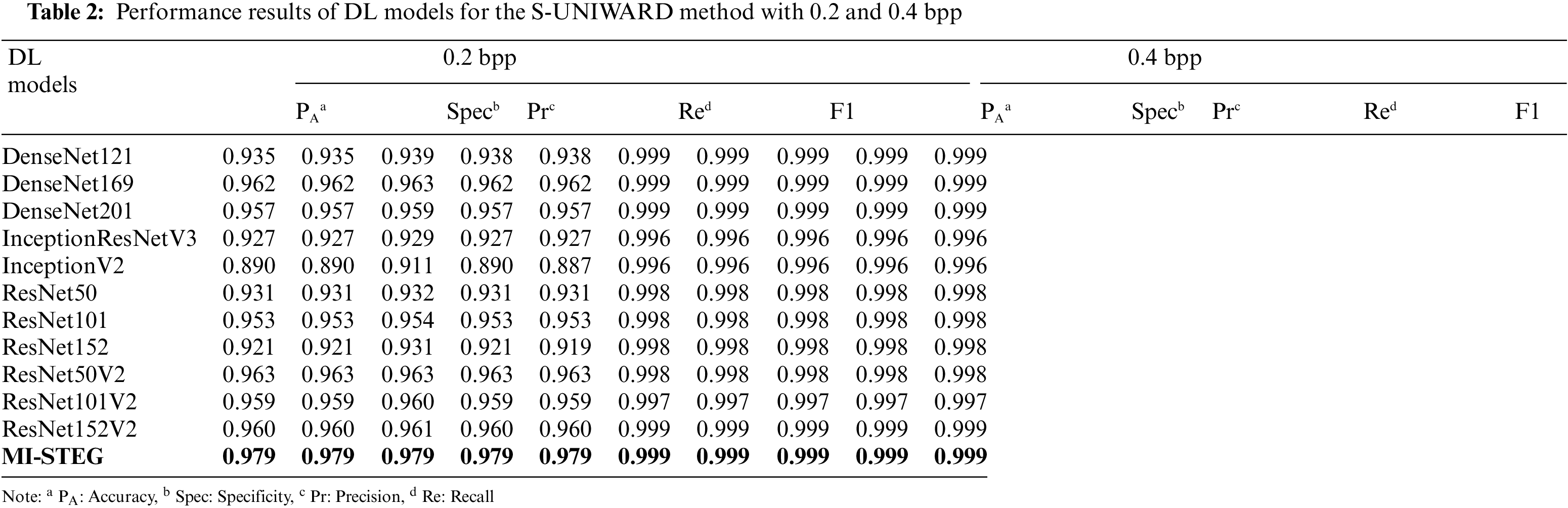
Fig. 5 shows the detection error and R values obtained by the DL models for detecting the S-UNIWARD method at various payloads. The detection error-values of the models for 0.1 and 0.2 bpp range from 0.193 to 0.366 and 0.021 to 0.214, respectively. The R values of the models for 0.1 and 0.2 bpp range from 0.456 to 0.634 and 0.800 to 0.958, respectively. The MI-STEG method achieved the lowest error and highest R values for all payloads.

Figure 5: Performance values of DL models for the S-UNIWARD method, a) detection errors, b) R values

Table 3 shows the detection performance results of DL models for the steganalysis MIPOD method with 0.2 and 0.4 bpp payloads. All models were successful in 0.4 bpp detection. ResNet architectures achieved slightly better results in detecting 0.2 bpp payload, while Inception models had the worst results. The MI-STEG model achieved the highest performance values.

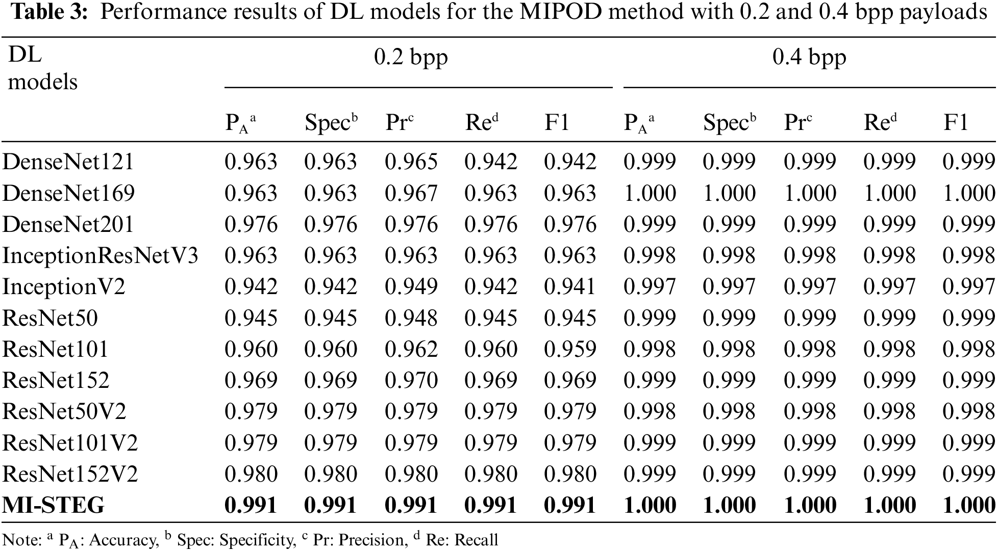
Fig. 6 presents the detection error and R values obtained by the DL models for detecting the MIPOD method at different payloads. The error values of the models for 0.1 and 0.2 bpp are in the 0.111 to 0.199 and 0.009 to 0.169 ranges, respectively. The R values of the models for 0.1 and 0.2 bpp range from 0.614 to 0.779 and 0.890 to 0.981, respectively. The MI-STEG method achieved the lowest error and highest R values for all payloads. These results clearly show that the study is highly innovative in the field of medical image steganography.

Figure 6: Performance values of DL models for the MIPOD method, a) detection errors, b) R values

4.2 Literature Comparison and Discussion

The literature is rich in studies on medical image steganography. However, studies focusing specifically on medical image steganalysis are rather rare. Ozcan et al. [40] developed an SVM classifier for the steganalysis of the hidden message in radiological images using the sequential LSB method. The inputs for SVM classification are obtained using the discrete cosine transform (DCT) proposed by Liu [41] and include 216 features. Although the study’s accuracy rate is 0.993, the feature extraction is quite costly. In another study [2], a CNN model with four convolution layers was developed for the steganalysis of the sequential LSB technique. The model’s accuracy was found to be 0.964. Even though these previous studies [2,40] have shown that medical image steganalysis can be performed with ML techniques, steganalysis based on the sequential LSB method is not compelling. In addition, as these studies employed the clairvoyant scenario, the images in the training and test datasets were produced on the same MR device. In contrast, the BOSSBase dataset used for image steganalysis includes images captured by seven different cameras.

The present study analyzed the LSB algorithm with a 1.0 bpp payload to create a base pre-trained model for the CNN models. All models detected the LSB method with 100% accuracy. In my previous work [10], the WOW technique, which is a difficult method of steganalysis, was adapted to medical images. The steganalysis performance levels of the Inception and Efficient models other than DenseNet, and ResNet, were examined. It was found that weight transfer between DL models for steganalysis with different payloads improved the detection accuracy. The DenseNet model’s partially maximum accuracy values for 0.2 and 0.4 bpp payloads were 0.876 and 0.992, respectively. However, the steganalysis performances of the TFL-based DL models were very close, except for the Efficient model. For this reason, this study evaluated the steganalysis of three distinct spatial embedding techniques with different payloads with an ensemble model combining eleven CNNs, leading to high-performance values for all three methods, as shown in Table 4.

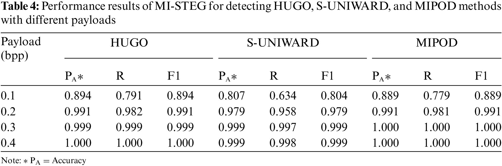
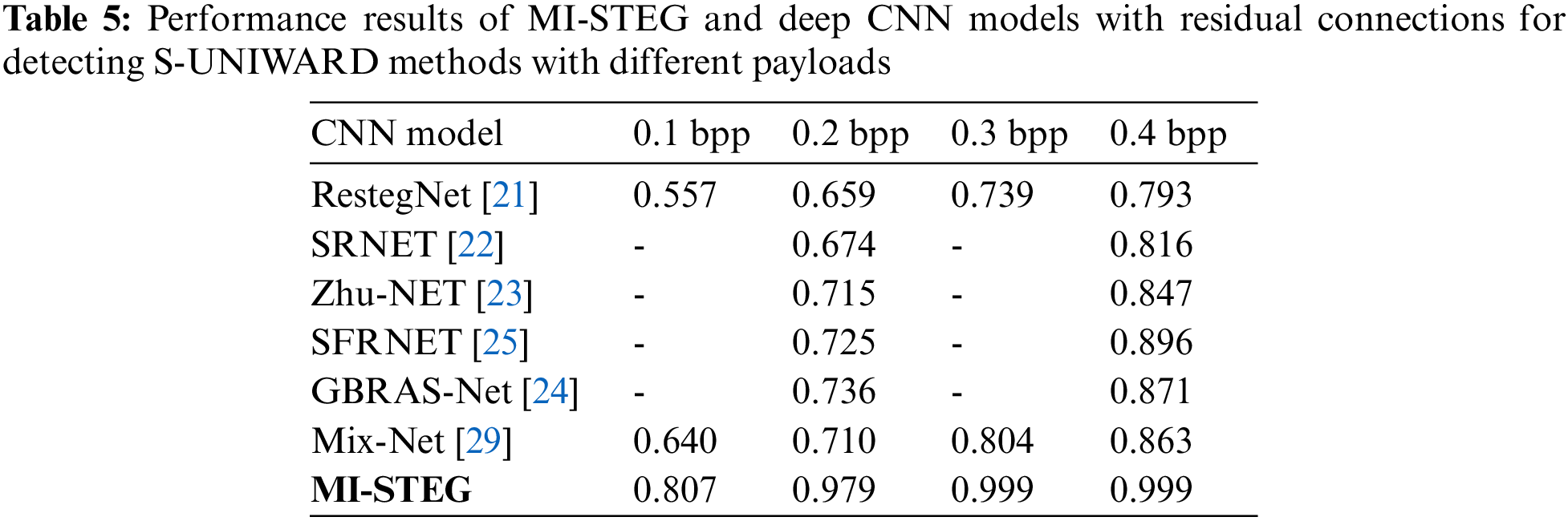
Table 5 shows the performance values of the MI-STEG and the deep CNN models suggested for the steganalysis of the S-UNIWARD method with 0.2 and 0.4 bpp payloads. These CNN models used the BOSSBase dataset for training and testing CNNs [21–24,29]. Although the same data sets are not used, the results given in Table 5 clearly show the steganalysis success of models using residual connections. In addition, an ensemble of the features of CNN models improved the steganalysis performance [29]. In this study, ResNet, DenseNet, and Inception models with residual connections were used. The results of these models were combined into an ensemble model to ensure that low-level stego noise is separated from the image content in deep layers. The model developed here is highly successful in medical image steganalysis with different payloads. However, while it is generally challenging to detect payloads below 0.4 bpp in image steganalysis, it appears particularly difficult to detect a 0.1 bpp payload in medical image steganalysis.

5  Conclusion

In light of previous studies on image steganalysis, this study establishes the limits of medical image steganalysis for the first time. In recent years, low stego noise in images has been detected using DL models, avoiding the costly feature analysis required by ML techniques for image steganalysis. In the literature, deep networks and ensemble models with residual links are recommended for the steganalysis problem. Against this background, this study proposes an ensemble CNN model, MI-STEG, which combines TFL-based ResNet, DenseNet, and Inception models for medical image steganalysis. A dataset comprised of axial, coronal, and sagittal slices of T1, T2, and FLAIR-weighted brain MR images obtained from three different centers were developed for the experiments. Doing so introduced a range of diversity of images, which were taken by seven distinct cameras at different angles and light settings as included in the BOSSBase dataset of medical images. Since the cover-stego mismatch scenario was adopted in the study, pre-trained models were evaluated using a different MR dataset. The proposed MI-STEG model detected HUGO, S-UNIWARD, and MIPOD embedding techniques with high accuracy, for each payload between 1.0 and 0.1 bpp. In this context, it was demonstrated that data maliciously hidden in medical images could be detected with DL models. Additionally, these DL models can contribute to developing new medical image steganography techniques.

Acknowledgement: I owe gratitude to Prof. Inan Guler from Gazi University, Ankara, Turkey, and Assoc. Prof. Burhanettin Cigdem from Cumhuriyet University, Sivas, Turkey, for sharing the data used in this article. I also would like to thank Kali Gurkahraman (Ph.D.) from Cumhuriyet University, Sivas, Turkey, for insightful discussions on the use of DL.

Funding Statement: The author received no specific funding for this study.

Conflicts of Interest: The author declares that they have no conflicts of interest to report regarding the present study.

References

1. R. Karakis, I. Guler, I. Capraz and E. Bilir, “A novel fuzzy logic based image steganography method to ensure medical data security,” Computers in Biology and Medicine, vol. 67, pp. 172–183, 2015. [Google Scholar]
2. R. Karakis and K. Gurkahraman, “Steganalysis with deep learning on medical images,” Journal of Information Technologies, vol. 14, no. 2, pp. 151–159, 2021. [Google Scholar]
3. J. Hussain, J. Zeng, Xinhong and S. Tan, “A survey on deep convolutional neural networks for image steganography and steganalysis,” KSII Transactions on Internet and Information Systems, vol. 14, no. 3, pp. 1228–1248, 2020. [Google Scholar]
4. K. Karampidis, E. Kavallieratou and G. Papadourakis, “A review of image steganalysis techniques for digital forensics,” Journal of Information Security and Applications, vol. 40, pp. 217–235, 2018. [Google Scholar]
5. A. Selvaraj, A. Ezhilarasan, S. L. J. Wellington and A. R. Sam, “Digital image steganalysis: A survey on paradigm shift from machine learning to deep learning based techniques,” IET Image Processing, vol. 15, pp. 504–522, 2021. [Google Scholar]
6. L. Pibre, J. Pasquet, D. Ienco and M. Chaumont, “Deep learning is a good steganalysis tool when embedding key is reused for different images, even if there is a cover source mismatch,” Electronic Imaging, vol. 2016, no. 8, pp. 1–11, 2016. [Google Scholar]
7. J. Fridrich and J. Kodovsky, “Rich models for steganalysis of digital images,” IEEE Transactions on Information Forensics and Security, vol. 7, no. 3, pp. 868–882, 2012. [Google Scholar]
8. S. Dumitrescu, X. Wu and Z. Wang, “Detection of LSB steganography via sample pair analysis,” IEEE Transactions on Signal Processing, vol. 51, no. 7, pp. 1995–2007, 2003. [Google Scholar]
9. S. Ge, Y. Gao and R. Wang, “Least significant bit steganography detection with machine learning techniques,” in Proc. DDDM, San Jose California, USA, pp. 24–32, 2007. [Google Scholar]
10. R. Karakis, “Medical image steganalysis using deep convolutional neural network,” in Proc. ICENTE’21, Konya, Turkey, pp. 88–92, 2021. [Google Scholar]
11. R. Benton and H. Chu, “Soft computing approach to steganalysis of LSB embedding in digital images,” in Proc. ITRE 2005, Hsinchu, Taiwan, pp. 105–109, 2005. [Google Scholar]
12. L. Shaohui, Y. Hongxun and G. Wen, “Neural network based steganalysis in still images,” in Proc. ICME ‘03 (Cat. No.03TH8698), Baltimore, MD, USA, vol. 2, pp. II–509, 2003. [Google Scholar]
13. L. Shaohui, Y. Hongxun and G. Wen, “Steganalysis based on wavelet texture analysis and neural network,” in Proc. WCICA (IEEE Cat. No.04EX788), Hangzhou, China, vol. 5, pp. 4066–4069, 2004. [Google Scholar]
14. S. Tan and B. Li, “Stacked convolutional auto-encoders for steganalysis of digital images,” in Proc. APSIPA, Siem Reap, Cambodia, pp. 1–4, 2014. [Google Scholar]
15. Y. Qian, J. Dong, W. Wang and T. Tan, “Deep learning for steganalysis via convolutional neural networks,” Media Watermarking, Security, and Forensics, SPIE, vol. 9409, pp. 171–180, 2015. [Google Scholar]
16. Y. Qian, J. Dong, W. Wang and T. Tan, “Learning and transferring representations for image steganalysis using convolutional neural network,” in Proc. ICIP, Phoenix, AZ, USA, pp. 2752–2756, 2016. [Google Scholar]
17. G. Xu, H. Wu and Y. Shi, “Structural design of convolutional neural networks for steganalysis,” IEEE Signal Processing Letters, vol. 23, no. 5, pp. 708–712, 2016. [Google Scholar]
18. J. Ye, J. Ni and Y. Yi, “Deep learning hierarchical representations for image steganalysis,” IEEE Transactions on Information Forensics and Security, vol. 12, no. 11, pp. 2545–2557, 2017. [Google Scholar]
19. M. Salomon, R. Couturier, C. Guyeux, J. F. Couchot and J. M. Bahi, “Steganalysis via a convolutional neural network using large convolution filters for embedding process with same stego key: A deep learning approach for telemedicine,” European Research in Telemedicine/La Recherche Européenne en Télémédecine, vol. 6, no. 2, pp. 79–92, 2017. [Google Scholar]
20. S. Wu, S. Zhong and Y. Liu, “Deep residual learning for image steganalysis,” Multimedia Tools and Applications, vol. 77, pp. 10437–10453, 2018. [Google Scholar]
21. W. You, X. Zhao, S. Ma and Y. Liu, “RestegNet: A residual steganalytic network,” Multimedia Tools and Applications, vol. 78, pp. 22711–22725, 2019. [Google Scholar]
22. M. Boroumand, M. Chen and J. Fridrich, “Deep residual network for steganalysis of digital images,” IEEE Transactions on Information Forensics and Security, vol. 14, no. 5, pp. 1181–1193, 2019. [Google Scholar]
23. R. Zhang, F. Zhu, J. Liu and G. Liu, “Depth-wise separable convolutions and multi-level pooling for an efficient spatial CNN-based steganalysis,” IEEE Transactions on Information Forensics and Security, vol. 15, pp. 1138–1150, 2019. [Google Scholar]
24. T. S. Reinel, A. A. H. Brayan, B. O. M. Alejandro, M. R. Alejandro, A. G. Daniel et al., “GBRAS-net: A convolutional neural network architecture for spatial image steganalysis,” IEEE Access, vol. 9, pp. 14340–14350, 2021. [Google Scholar]
25. G. Xu, Y. Xu, S. Zhang and X. Xie, “SFRNet: Feature extraction-fusion steganalysis network based on squeeze-and-excitation block and RepVgg block,” Security and Communication Networks, vol. 2021, no. 3676720, pp. 1–11, 2021. [Google Scholar]
26. S. Ozcan and A. F. Mustacoglu, “Transfer learning effects on image steganalysis with pre-trained deep residual neural network model,” in Proc. Big Data, Seattle, WA, USA, pp. 2280–2287, 2018. [Google Scholar]
27. J. Butora, Y. Yousfi and J. Fridrich, “How to pretrain for steganalysis,” in Proc. IH&MMSec’21, Brussels, Belgium, pp. 143–148, 2021. [Google Scholar]
28. G. Xu, H. Z. Wu and Y. Q. Shi, “Ensemble of CNNs for steganalysis: An empirical study,” in Proc. IH&MMSec’16, Vigo, Galicia, Spain, pp. 103–107, 2016. [Google Scholar]
29. E. Amrutha, S. Arivazhagan and W. Sylvia Lilly Jebarani, “MixNet: A robust mixture of convolutional neural networks as feature extractors to detect stego images created by content-adaptive steganography,” Neural Processing Letters, vol. 54, no. 2, pp. 853–870, 2022. [Google Scholar]
30. V. Holub and J. Fridrich, “Designing steganographic distortion using directional filters,” in Proc. WIFS, Costa Adeje, Spain, pp. 234–239, 2012. [Google Scholar]
31. G. Huang, Z. Liu, L. Van Der Maaten and K. Q. Weinberger, “Densely connected convolutional networks,” in Proc. CVPR, Honolulu, HI, USA, pp. 4700–4708, 2017. [Google Scholar]
32. K. He, X. Zhang, S. Ren and J. Sun, “Deep residual learning for image recognition,” in Proc. CVPR, Las Vegas, NV, USA, pp. 770–778, 2016. [Google Scholar]
33. C. Szegedy, V. Vanhoucke, S. Ioffe, J. Shlens and Z. Wojna, “Rethinking the inception architecture for computer vision,” in Proc. CVPR, Las Vegas, NV, USA, pp. 2818–2826, 2016. [Google Scholar]
34. R. Karakis, K. Gurkahraman, B. Cigdem, I. Oztoprak and A. S. Topaktas, “Evaluation of segmented brain regions for medical image steganography,” Journal of the Faculty of Engineering and Architecture of Gazi University, vol. 36, no. 4, pp. 2301–2314, 2021. [Google Scholar]
35. Internet: “Figshare brain tumor dataset,” [Online]. Available: https://doi.org/10.6084/m9.figshare.1512427.v5. (accessed on 27 September 2022). [Google Scholar]
36. I. Goodfellow, Y. Bengio and A. Courville, “Convolutional networks,” in The Deep Learning (Adaptive Computation and Machine Learning), 1st ed., vol. 1, Cambridge, Massachusetts, USA: MIT Press, pp. 326–366, 2016. [Google Scholar]
37. A. Krizhevsky, I. Sutskever and G. Hinton, “ImageNet classification with deep convolutional neural networks,” in Proc. NIPS’12, Nevada, USA, vol. 1, pp. 1097–1105, 2012. [Google Scholar]
38. K. Gurkahraman and R., Karakis, “Brain tumors classification with deep learning using data augmentation,” Journal of the Faculty of Engineering and Architecture of Gazi University, vol. 36, no. 2, pp. 997–1011, 2021. [Google Scholar]
39. J. Gu, Z. Wang, J. Kuen, L. Ma, A. Shahroudy et al., “Recent advances in convolutional neural networks,” Pattern Recognition, vol. 77, pp. 354–377, 2018. [Google Scholar]
40. F. B. M. Ozcan, R. Karakis and I. Guler, “Steganalysis on medical images with support vector machine,” in Proc. SIU, Gaziantep, Turkey, pp. 1–4, 2020. [Google Scholar]
41. Q. Liu, “Steganalysis of DCT-embedding based adaptive steganography and YASS,” in Proc. MM&Sec ‘11, Buffalo, New York, USA, pp. 77–86, 2011. [Google Scholar]
Cite This Article
Copyright © 2023 The Author(s). Published by Tech Science Press.
This work is licensed under a Creative Commons Attribution 4.0 International License , which permits unrestricted use, distribution, and reproduction in any medium, provided the original work is properly cited.
Downloads
Citation Tools