Data Augmentation and Random Multi-Model Deep Learning for Data Classification

1  Introduction

In the data science community, classification and categorization using complex data of images, video and documents are crucial challenges. In recent years, there has been a growing interest in applying DL structures and architectures to such problems.

However, popular deep architectures are intended specifically for data type or domain. Therefore, there is an essential need to improve further information handling approaches for categorization and classification through an extensive variety of data types.

Even though DL has been successfully utilized to solve classification problems [1] the key issue is deciding which DL architecture such as Deep Neural Network (DNN), Convolutional Neural Network (CNN) or Recurrent Neural Network (RNN) to use for a given task. Several nodes (units) and hidden layers are also very useful for varied data kinds and application structures. Hence, the best way to solve this issue is by trial and error method for the application or dataset.

The difficulty of deploying ensembles of deep architectures is addressed in this paper with a method known as RMDL [2]. In short, RMDL is a method that incorporates three DL architectures: CNN, DNN and RNN. Experiments with numerous sorts of data have shown that this method is accurate, dependable and efficient.

For their input layers, the three basic DL designs use various feature space techniques. DNN, for example, extracts features from the text using frequency-inverse document frequency (TF-IDF) [3]. RMDL uses randomly generated hyper-parameters to find the number of both hidden layers and nodes (density) in each DNN hidden layer. By using random feature maps and random numbers of hidden layers, RMDL selects hyper-parameters in CNN.

The CNN structures used by RMDL are 1-dimensional CNN (Conv1D) which only moves along a single axis so it used for text, a 2-dimensional CNN (Conv2D) which works by applying kernels that strides along 2-dimensional space so it used for picture. In 3-dimensions CNNs (Conv3D) the kernels move in three dimensions so it is suitable for video processing [1]. Text classification is primarily accomplished using RNN architectures. The RMDL model employs two RNN structures: Gated Recurrent Units (GRUs) and Long Short-Term Memory (LSTM). As a result, the RMDL’s number of GRU or LSTM and the hidden layers are determined through a search of randomly generated hyper-parameters [1].

The rest of the paper is organized as follows; Section 2 gives the related works. The proposed approach for data augmentation using GANS is described in Section 3. Section 4 discusses an approach for text augmentation. Section 5 presents an overview for RMDL that used for classification. The experimental results are elaborated in Section 6, Finally, Section 7 is the Conclusion of the paper.

2  Related Works

Generally, for the validation and test sets, the model does not generalize well if trained using a small set of samples. Therefore, such models may suffer from the overfitting problem. Numerous approaches have been proposed to reduce overfitting [4]. The simplest method is to add a regularization term on the weight’s norm. An additional common technique employed is a dropout.

Probabilistically, dropout is a workaround in case the lesser computation is the target as such the neurons (units) are dropped randomly in the training process. It enables neurons to be independent as units are randomly dropped. At test time, this has the averaging effect on the predictions over several networks [5,6]. In [7], the authors show that dropout attains superior results on various test datasets.

Batch normalization is another common technique to avoid the model’s overfitting; it normalizes layers and permits training of the normalization weights. Within the network, batch normalization can be applied on any layer and therefore it works effectively. Particularly when it is utilized in GANs [8] such as CycleGAN in [9]. Furthermore, transfer learning is a method of efficiently solving an issue by training neural net pre-trained weights on some relevant or more broad data and suitable parameters.

Previous research to systematically understand the benefits and limitations of data augmentation demonstrate that data augmentation can act as a regularizer in preventing overfitting in neural networks [10].

Data augmentation is not a novel field and several data augmentation methods have been applied to explicit problems. Data augmentation is the procedure of increasing the training dataset by creating more samples taking advantage of the training data.

There are several approaches to augment data. Geometric transformations and color augmentation are famous approaches when using images to increase dataset size. Smart Augmentation (SA) [11] and Neural Augmentation (NA) [12] have been proposed in recent years for similar tasks. During the training of the target network, smart augmentation creates a network that is learned to generate augmented data such that the loss of the target networks is minimized.

NA behaves like SA such that they separate networks to perform data augmentation which improves the classifier. However, NA uses pair of images randomly selected from the same class as an input. Manual data augmentation and data augmentation through training neural networks are the two main types of data augmentation approaches. Different neural network topologies, on the other hand, can be employed in data augmentation by training neural networks. The focus of this paper is on GANs.

Artificially, augmentation in image classification methods generates training images by altering available images [13]. Classification tasks take benefit of the augmentation of many images. The structure of images is changed to enhance the number of samples available to the ML algorithm, while flexibility is included in the final model [14].

As such, data augmentation techniques belong to the category of data warping, a method that searches directly to augment the input data to the data space. The idea of augmentation was accomplished on the MNIST dataset in [15]. A very common and conventional method to augment image data is to achieve geometry and augmentations of color, such as image reflecting, translating, cropping of the image, and changing the palette of image color as in [13,16]. The performance of classifiers on the MNIST database has been improved over elastic deformation’s introduction in [17], additionally using the existing affine transformations.

In [18], a method called neural augmentation is proposed to allow a neural net to learn augmentations which improve the ability to correctly classify images. They proposed two different approaches to data augmentation. The first approach is generating augmented data before training the classifier by applying GANs and basic transformations to create a larger dataset. The second approach attempts to learn augmentation through a prepended neural net. AutoAugment [19], developed by Cubuk et al., is a much different approach to meta-learning than Neural Augmentation or Smart Augmentation. AutoAugment is a Reinforcement Learning algorithm that searches for an optimal augmentation policy amongst a constrained set of geometric transformations with miscellaneous levels of distortions.

Data augmentation techniques generally fall under two categories: Firstly, data augmentation by manual approaches, and secondly, using neural networks. In this paper, we particularly emphasize using GANs. In this approach, new data samples are generated from the distribution, which is learned from already available data. Therefore, we believe that it is a good alternative compared to manual augmentation.

3  Generative Adversarial Networks (GANs)

In fields like Computer Vision (CV), the GANs have been excessively employed to generate new images for training. Moreover, even with relatively insignificant sets of data, GANs have been effective by learning techniques as in [20]. Single neural net produces better counterfeit examples from the original distribution of the data using a min-max strategy to trick the other net. Subsequently, the other net is trained to differentiate the counterfeits better. For style transfer in CycleGAN, GANs are used as image transferring from one setting to another. Furthermore, at augmenting datasets, GANs have shown to be very effective such as in increasing the input images resolution [21]. Infrequent instances, GANs have accomplished a lot of success.

The framework in [22] attains good overall performance on the datasets MNIST [23], CIFAR-10 [24] GANs have also proven effective in instance paragraph generation [25]. The proposed system in [26] has achieved good results using CNN. CNNs can effectively extract and learn a huge number of features. The superior performance of the CNNs is related to the sparse connections between neurons with several variables in these networks being low.

A generator G model and a discriminator D model are common in GANs. The generator learns the dataset G distribution gap. The discriminator D determines if the data comes from a true distribution or a gap. The discriminator D distinguishes between actual and synthetic images when it comes to visuals. The generator G aids in the creation of natural-looking photographs. While the generator is attempting to deceive the discriminator, the discriminator is attempting to avoid being deceived by the generator. GANs have been found to be particularly unstable for training, resulting in generators that produce insufficient outputs.

To overcome this problem, in this paper, we introduce the advantage of using Deep Convolutional Generative Adversarial Networks (DCGAN). Based on these generative models, a hierarchy of abstract features can be learned from parts of objects in the scene. As such, the learned features can characterize the distribution of underlying data and samples, which have been generated from these features, are common in real-world scenarios. Significantly, DCGAN achieves good results mostly because of the stability of its architecture in training which affects the quality of the samples. Both the generator and discriminator models in DCGAN are CNNs rather than multilayer perceptron.

In this paper, we describe a method for augmenting data using DCGAN. Through a range of datasets, the proposed framework trains GANs which leads to stable training. Mainly, our proposed framework relies on three modifications in the architecture of CNN. Traditionally in every layer of CNN, a pooling layer follows convolutional layers. Practically, applying pooling is to down-sample the previous input. Nonetheless, later, it is validated that getting all convolutional layers and getting the network to train its spatial downsampling improves the performance of CNNs. Thus, this is the first interesting contribution to the proposed architecture.

Generally, neural network architecture is achieved by creating CNN layers block, followed by stacked fully connected layers. With each node in the layer, the latest layer is fully connected which has a Softmax activation function specifying the image probability of a specific class. As such, the fully connected layers have abundant parameters resulting in overfitting. Thus, dropout is used to avoid overfitting.

Recently, to reduce overfitting global average pooling is proposed in which parameters number in the network is reduced. Global average pooling reduces spatial dimensions in a similar manner as the max-pooling technique, but the global average-pooling technique reduces the dimensions very efficiently. Simply, by taking an average of WH values, W×H×d tensor is converted to 1×1×d. To calculate the probability on this layer, the soft-max activation function is applied. This will be the second contribution to our architecture.

Nevertheless, the stability of the model is increased by global average-pooling which hits the speed of convergence. In [22], the authors proposed to connect the maximum features to the generator and the discriminators’ input and output respectively. Commonly while GANs training, the generator collapses to generate samples from the same point. Hence, to avoid this problem we suggested using batch normalization. To achieve unit-variance and zero-mean, the batch normalization approach normalizes the input for each unit. Thus, this allows treating with poor initialization problems and similarly reliefs vanishing addressing, explosion and further gradient descent problems. This is the third contribution to our architecture.

As mentioned already, the generation of high-resolution images by GANs modeling is an unstable procedure. Consequently, selecting the same architecture for generator and discriminator for diverse datasets by varying images resolutions is illogical. Therefore, our architecture is modeled in such a manner that CNN layers’ number in generator and discriminator are contingent on images resolution. Several convolutional layers in the generator are calculated as:

num_of_layers=(heightofimage)−2(1)

Contrariwise, the number of the convolutional layers in the discriminator is calculated as (num_of_layers)+1. A vector drawn from the normal or uniform distribution is used as the generator input. As a result, the initial layer in a generator architecture can be a completely connected layer with a matrix multiplication. As a result, the layer’s output is reformed into a four-dimensional tensor. Batch-normalization was previously used on the 4-dimensional tensor. The tensor obtained works as a surprise of the convolution stack having size m×4×4×c where m represents the number of images in batch size heuristically, c is the features of the convolutional number which is computed as:

c=128∗(num_of_layers−1)(2)

It is expected for each convolutional layer to take a tensor of the following form for the last layer in the stack:

n×[4∗layer_number]×[4∗layer_number]×[c/2^(layer_number−1)](3)

where the tensors’ input and outputs are of the form:

n×[4∗(layer_number+1)]×[4∗(layer_number+1)]×[f/2^(layer_number)](4)

where: layer_number=1…((num_of_layers)−1). Noticeably, in each layer, the height and width are up-sampled by factor two such that the features number is also down-sampled by factor two. The transpose of a convolution layer is upscaled for each convolutional NN, with a kernel of size 5-by-5 by two strides for vertical and horizontal directions.

Subsequently, it is required to carry out batch-normalization for the output of each convolutional layer before taking it as the following CNN layer input. Thus, the last layer in the convolutional stack yields an output of size m×s×s×f where f is the channels number inside the image and s is the image size. Hence, batch-normalization is not carried out on the final layer so that oscillation of the sample can be avoided, and stability of the model is maintained. Lastly, tanh activation-function is applied to the output which is handled as generated models.

An image is taken as input to discriminator which has size m×s×s×f. Additionally, the discriminator only has one more convolutional layer rather than the layers’ number in the generator. In the proposed architecture, the first layer is a convolutional layer. So, instead of decreasing dimensions in this layer of input, further feature maps are produced. More accurately, this layer output is represented of size m×s×s×64.

To avoid overfitting, dropout is applied to this layer output. Finally, the remaining convolutional layers are stacked taking input of the form: n×[s/(2∗(layer_number−1))]×[s/2∗(layer_number−1)]×64∗(layer_number−1)

where input and outputs yield a tensor of the form:

n×[s/(layer_number∗2]×[s/(2∗(layer_number−1)))]×[layer_number∗64](5)

where layer_number=2…(num_of_layers+1). For each layer, the generator height and width are up-sampled with factor two and the features number is down-sampled with a factor two. Furthermore, in each layer, the height and width of the discriminator are down-scaled by two and the features number is up-scaled with factor two.

Considerably, the proposed architecture is exhibited such that the convolutional layers’ highest number are connected respectively to generators’ and discriminators’ input and output. Convolution is applied in the vertical and horizontal directions from second convolutional layer to downscale using a 3 × 3 kernel with a step of two. In case of generator batch-normalization is carried out for each convolutional layer output. Moreover, dropout is applied in the last convolutional layer for all layers before been passed as input to CNN layer. In the convolutional stack, the last layer yields an output which has the following size representation 64×m×4×4∗(num_of_layers+1).

From last convolutional layer, for the resulting output, global average-pooling is applied in of size m×1×1×64∗(num_of_layers+1). In the proposed architecture, the final layer is a fully connected layer and this layer output is a matrix representation that has size m×(k+1). Finally, on output from this layer, soft-max activation function is applied which estimates an image probability to belong k+1 different classes. Algorithm 1 describes the proposed data augmentation using GANs.

At training time, training batch is generated from a batch of images then this image is fed into RMDL to do classification. Subsequently, randomly from the same class, two images are sampled and served as an input to augmentation network to generate the successive augmented image.

4  Text Augmentation

Text augmentation approaches have different factors associated with them for creating robust models. Some of the text augmentation techniques are more dependent on the details of the language [27] while other techniques do not require much detail if a model based on language is provided [28].

The models of semantic data have improved over the past few years with the aid of distributed word embedded representations [29]. New approaches for text understandability have been created such as text classification approaches as deployed in this research. The text augmentation techniques can be deployed for improving classification accuracy and creating robust models. This way, the classification models can be trained with a lesser requirement for labeled data.

The process of data labeling is very time and efficiency costly. Scenarios such as identification of fake news [30], getting the context of political news, public response on administration services [31], or crucial scenarios such as emergencies where better coordination is required, aptly labeled data is very difficult to attain. ML techniques require a huge amount of data to perform well and give optimal results. Such big data are available and accessible to big organizations along with the resources for labeling such data, but small organizations do not have such resources or access to data.

The changes in input data affect the performance of the classifier but for a robust classifier, it is required to have an ability to handle the data changes and have a learned model that gives a good response to input distribution changes. The reason for data changes in the evolution of language and changes in geographical aspects. Another use is semi-supervised learning, in which we use the few labels we must generate a noisy classifier that labels more unlabeled data before feeding it back to train another classifier.

This work introduces a text augmentation system that replaces terms that are used similarly from a global perspective rather than a context-specific perspective. So, rather than focusing on what the ideal word to replace in this sentence in this paper is, consider how similar words are utilized throughout texts. We further assess the proposed technique on various classification data.

Limited data is an issue when it comes to acquiring well-labeled data for supervised learning tasks [32], and it is even more of a problem for low-resource languages [33]. The augmentation effect on learning for DNN models is demonstrated here.

We employ pre-trained word vector representations from Glove [34] for the DNN. For the AG News dataset, the pre-trained Wikipedia model is utilized, and for the social media datasets, the pre-trained Twitter model is used. We augment the data five times across all the datasets in this experiment. We also incorporate the original dataset, resulting in a six-fold enlarged dataset. When no augmentation is used, we simply rerun the original dataset six times to make the findings similar.

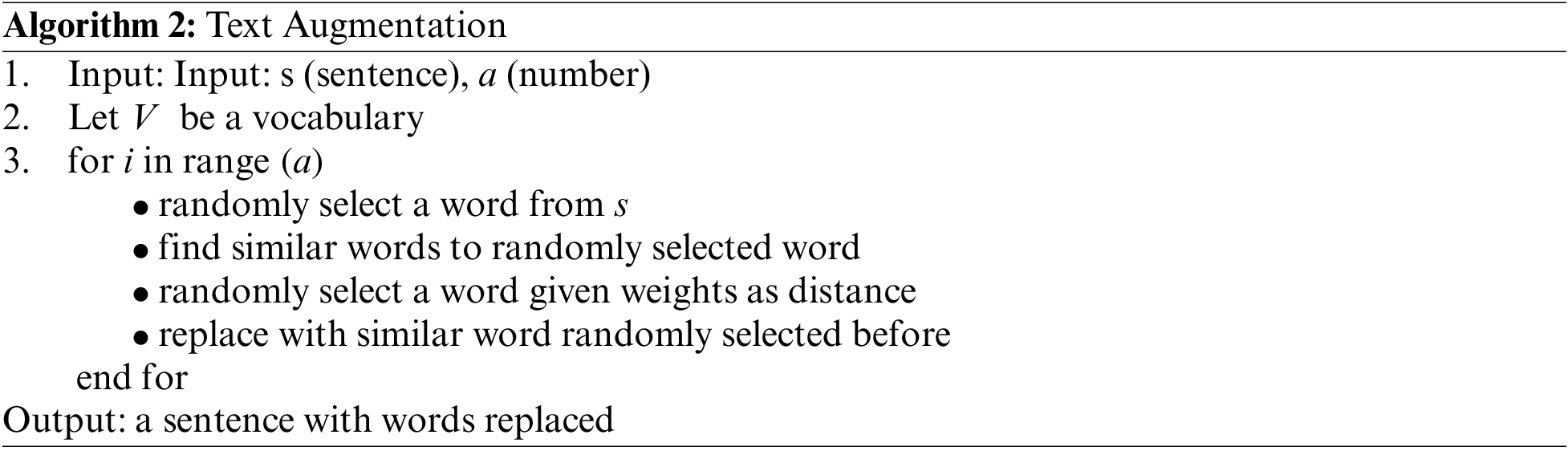
Word2vec-based augmentation (learned semantic similarity) Word2vec is a strong augmentation method that uses a word embedding model [29] trained on the public dataset to locate words that are mostly similar to a particular input word. We use a pre-trained Wikipedia Word2Vec model for formal text. To convert a Glove model pre-trained on Twitter data to Word2vec format for social media data, we employ Gen-sim [35]. The updated models are used in the proposed strategy to augment data by randomly assigning a word in a sentence and utilizing cosine similarity to determine the distributed representations of words and phrases as well as their compositionality. When selecting a comparable phrase, we use the cosine similarity as a relative weight to find a term that replaces the input word.

We are provided with a string and an integer in Algorithm 2, where the string represents the input data and the integer represents the number of repeats to supplement that data. Word2vec has the advantage of producing more contextually connected vectors, which means that words with similar meanings can be expressed accordingly.

We send the updated data (picture or text) into RMDL, which does categorization.

5  Random Multi Model Deep Learning

Multi random DL models [2] including DNN, RNN, and CNN techniques (or GRU) are used for text and image categorization. We’ll go over RMDL first, followed by the three DL architecture techniques (DNN, RNN, and CNN). The usage of multi optimizer methods in various random models will next be examined.

Multi-model random DL is a one-of-a-kind technique that involves training a large number of DNN, Deep CNN, and Deep RNN at the same time. The number of layers and nodes are produced for all of these deep learning multi-models (for instance, nine random models in RMDL consist of three CNNs, three RNNs, and three DNNs, such that all of them are unique owing to the random creation).

M(yi1,yi2,…,yin)=[12+(∑j=1nyij)−12n](6)

where n is random models’ number, and yij is the prediction of model output for data point i in model j Output space employs majority vote for final y^i. Hence, y^i can be expressed as follows:

y^i=[y^i1.…y^ij…y^in](7)

where n is random models’ number, and y^ij illustrates the document prediction of label either for document or data point of Diϵ{xi,yi} for model j and y^ij is defined as follows:

y^ij=[softmax(yij)](8)

After all of RDL’s models (RMDL) have been trained, the final forecast is made using the majority vote of these models.

5.1 Deep Learning in RMDL

The RMDL model structure contains three basic techniques of DL in parallel. In what follows, every individual model will be described separately. Consequently, the final model consists of d random DNNs, RNNs, and CNNs models.

5.2 Deep Neural Network

Layer multiconnection is used to learn the structure of DNNs, where each layer receives only connections from the preceding layer and only grants connections to the subsequent layer in hidden layers. This layer input is a link between feature space and all random models’ initial hidden layer. As a result, the output layer for multi-class classification is the number of classes, whereas for binary classification it is individual output.

In this paper, DNNs are trained several times for different purposes. In our proposed technique, multi-classes DNNs learned models are generated randomly. For instance, nodes number in each layer and furthermore layers’ number are entirely random assigned.

In our approach, DNNs are discriminative trained models that use sigmoid Eq. (9) and ReLU [36] as activation functions in a typical back-propagation algorithm. Finally, Softmax (11) should be used in output layer for classification of multi-class.

f(x)=11+e−xϵ(0,1)(9)

f(x)=max(0,x)(10)

σ(z)j=ezj∑k=1Kezkjϵ{1,…,K}(11)

Mainly, the goal is to learn from a set of example pairs (x, y), xϵX, yϵY, and target spaces using hidden layers. On the other hand, in classification of text, the input is string that is created by text vectorization.

5.3 Recurrent Neural Networks

Additional neural network architecture which contributes in RMDL model is RNNs. Practically, RNNs assign extra weights to the earlier sequence data points. Consequently, this procedure is a worthy method for classification of text, string and sequential data. Furthermore, in this work this procedure could be used for classification of images. RNN the neural net cogitates the previous nodes information which allows improved analysis of semantic for dataset structures. At step t, the formulation of this notion is given in Eq. (12) such that xt is the state on time t and ut denotes the input.

xt=F(xt−1,ut,θ)(12)

More explicitly, weights can be used to formulate Eq. (12) with specified parameters in Eq. (13):

xt=Wrecσ(xt−1)+Winut+b(13)

where Wrec indicates recurrent matrix weight, Win refers to weights of the input, b is the bias and σ denotes an element-wise function. Once more, the basic architecture for RMDL model is modified. Even though benefits of RNN, it has two major problems, first, when the gradient descent algorithm error is back propagated over the network and the second problem is vanishing gradient and exploding gradient [37].

In this paper, we have used the Gated hidden unit proposed by Choet al. (2014a), for RNN activation function σg. Simply, as an elementwise tanh, the gated concealed unit is an alternative to ordinary units. The gated unit is like Hochreiter and Schmidhuber’s (1997) long short-term memory (LSTM) unit, which can learn and model with long-term dependencies more effectively. Probably, this can be done by taking paths of computation within the unfolded RNN such that the derivatives product is close to one. By the way, these paths permit gradients to easily flow backward deprived of excessively suffering from the vanishing effect (Pascanu et al., 2013a). Consequently, it is potential to use LSTM units as an alternative to the gated hidden unit described but with some modification to the new state. The RNN new state si taking on n gated hidden units is calculated as follows:

si=σg(si−1,yi−1,ci)=(1−zi)∘si−1+zi∘si(14)

where σg is an element-wise multiplication, and zi is the update gates output. We have used the following updated state si which is computed by:

s~i=tanh tanh(We(yi−1)+U[ri∘si−1]+Cci)(15)

where e(yi−1)ϵn is an n-dimensional word yi−1 embedding, and ri is the retuned gates output. Such that yi is represented as a 1−of−M vector, simply e(yi) is a column of an embedding matrix E ϵ Rn×M. Occasionally, bias terms are omitted to get equations which are less muddled. The update gate zi allows each hidden unit to keep its preceding activation, such that the reset gate ri which controls the information quantity which should be rest from the previous state. This is computed as follows:

zi=σ(Wze(yi−1)+Uzsi−1+Czci)(16)

ri=σ(Wre(yi−1)+Ursi−1+Crci)(17)

where W,U represent parameter matrices and σ(.) is a logistic sigmoid function.

5.4 Convolutional Neural Networks (CNN)

The final DL technique that contributes to RMDL is CNNs developed for hierarchical document or picture classification. The basic CNN convolves a tensor of the image with a set of kernels of size dd for image processing. The feature maps are convolutional layers that can be stacked to offer different input filters. Pooling is a technique used in CNN to decrease computational complexity by lowering output size from one layer to the next. We employ global average pooling to reduce overfitting by lowering the number of parameters in the network. The maps are converted to columns so that the output from the stacked featured maps can be fed into the next layer.

The final layers of a CNN are usually fully connected. During the backpropagation step of a CNN, not only the weights but also the feature detector filters are modified. The channels number, which reflects the feature area size, is, on the other hand, a major challenge for CNN when it comes to text. Practically, the CNN dimensionality for text is high.

5.4.1 Optimization

In this paper, we used two stochastic gradient optimizers in implementation of NNs that are Adagrad and Adadelta. Adagrad is addressed in [38] which are sub gradient methods, dynamically it absorbs geometry data knowledge to achieve more helpful the gradient based on learning. In iteration k, define:

G(k)=diag[∑i=1kg(i)(g(i))T]12(18)

Diagonal matrix:

Gjj(k)=∑i=1k(gi(i))2(19)

Update rule:

x(k+1)=argargminxϵX{<∇f(x(k)),x>+12αk‖x−x(k)‖G(k)2}(20)

=x(k)−αB−1∇f(x(k))(ifX=Rn)(21)

AdaDelta is introduced by MD. Zeiler [39] as an updated version of Adagrad. This method uses decaying average of gt exponentially as 2nd gradient moment. In fact, this method depends on only first order. For Adadelta, the update rule is as follows:

gt+1=γgt+(1−γ)∇L(θ)2(22)

xt+1=γxt+(1−γ)vt+12(23)

vt+1=−xt+ϵδL(θt)gt+1+ϵ(24)

5.4.2 Multi Optimization Rule

Practically, if one optimizer does not offer a good fitting for an explicit dataset, the RMDL using multi model has n random models. Such that some of them might utilize various optimizers which could disregard k models that are not effective if and only if n > k. In this paper, we only utilized two optimizers (Adagrad, and Adadelta) for the model evaluation, however the RMDL model can utilize slightly other optimizer.

6  Experimental Results

This section provides comprehensive experiments on the efficacy of classification using data augmentation techniques. The results indicate that using neural augmentation is more precisely using GANs. At training time, the MNIST [23] and CIFAR-10 [24] datasets are used experimentally with GANs. On CIFAR-10 and MNIST, GANs were trained for 200 and 140 k iterations, respectively. Alternatively, at each iteration, the generator and discriminator losses are fixed. For training, Adagrad and Adadelta optimizers are employed, which incorporate shifting parameter averages, allowing for larger effective steps and hence faster convergence.

In order to improve performance and reduce training time, the learning rate should be reduced when training grows. As a result, the learning rate will be based on an exponential decay. The exponential decay is calculated as:

decayedlearningrate=learningrate∗decayrate∗(globalstepdecaysteps)(25)

where initial learning rate, rate of decay, iteration number, and decay number steps are starting learning rate, rate of decay, global step, and decay steps, respectively.

Initial learning is set to 0.01, number of decay steps to 20000, and decay rate to 0.1 in our model. In both generator and discriminator, a used batch size is 128. To avoid overfitting, dropout is used in discriminator architecture. In our experiments, a dropout probability employed is 0.05. Input to the generator is a latent space variable of 100.

6.1 Evaluation

In this paper, the accuracy and Micro F1-Score are given as follows:

Precisionmicro=∑l=1LTPl∑l=1LTPl+FPl(26)

Recallmicro=∑l=1LTPl∑l=1LTPl+FNl(27)

F1−Scoremicro=∑l=1L2TPl∑l=1LTPl+FPl(28)

The performance of the proposed model is assessed in terms of F1-score and error rate for accuracy evaluation. Formally, given I={1,2,…,k} a set of indices, we define the ith class as Ci. We denote TPi_true positive of Ci,TPi_false positive, TNi_false negative, TNi_true negative counts respectively.

6.2 Experimental Setup

For testing and evaluating the performance of our approach, two datasets type one for text and the other for image have been used. Nevertheless, the model has ability to solve problems of classification using different data such as video, images, and text.

6.2.1 Image Datasets

For all these experiments, we used MNIST [23] and CIFAR-10 [24] datasets. We briefly describe characteristics of the datasets before proceeding to experiments. The CIFAR-10: The tagged photos are a subset of the 80 million Tiny labeled images dataset. The data collection contains images from ten different classes. Automobile, Airplane, Bird, Cat, Dog, Deer, Frog, Truck, Horse and Ship are the categories in which all the images fall. Interestingly, the groups are mutually exclusive.

Each class has 6000 images in the CIFAR-10 dataset, which has 60000 32 × 32 color images. In practice, this dataset is split into two parts: training data with 50000 images and testing data with 10000 images. Contrariwise, MNIST dataset comprises handwritten digits’ images. In the MNIST database, there are 70000 handwritten digits. The photos are 28 × 28 in size and are divided into ten categories. There are 50000 images in the training data and 10,000 images in the testing data in this dataset. Because all the photos in both datasets are the same size, data pre-processing was minimal, except for normalizing the images.

6.2.2 Text Datasets

Practically, four different datasets have been used for text classification, namely; WOS, Reuters, IMDB and 20 newsgroups. A collection of academic articles’ abstracts named Web of Science (WOS) [40] dataset consists of three corpora (5736, 11967, and 46985 documents) for (11, 34, and 134 topics). The Reuters-21578 news dataset includes 10,788 documents distributed into 7,769 documents used for training and 3,019 for validation through 90 classes totally.

IMDB dataset comprises 50,000 reviews divided into 25,000 highly widely set held reviews of movie used for training, and a set 25,000 for validation. 20 NewsGroup dataset contains 19,997 documents which its maximum length is 1,000 words. For this dataset, there are 15,997 used for training and 4,000 for testing.

6.2.3 Framework

The suggested framework is implemented in Python using a parallel computing platform and Application Programming Interface (API) paradigm established by Nvidia known as Compute Unified Device Architecture (CUDA). Finally, TensorFlow and Keras library have been used for the neural network creation [41].

6.3 Empirical Results

In this paper, execution of all shown results are performed on Central Process Units (CPU) and Graphical Process Units (GPU). Correspondingly, RMDL can run on either GPU, CPU, or composed. The processing unit used in these experiments is intel on Xeon E5-2640 (2.6 GHz) with 12 cores and 64 GB memory. Moreover, three graphical cards have been used which are two NVidia GeForce GTX 1080 Ti and NVidia Tesla K20c.

Before proceeding to experiment results, it is required to generate training batches. We only used a subset of the datasets as training data in practice. More specifically, the training data for CIFAR-10 and MNIST contains 5000 images, 500 of which belong to each of the 10 classes, while the testing data, which contains 10,000 images, remains unchanged. The experimental results of RMDL are shown in text categorization and image classification.

6.3.1 Image Classification

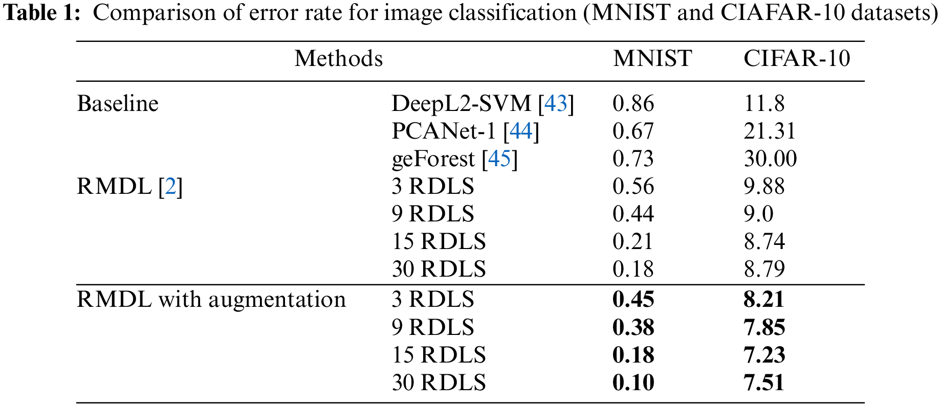
The baselines used for image classification are: Deep L2-SVM [42], PCANet-1 [43], gcForest [44] and RMDL with no augmentation. Table 1 shows the RMDL error rate for images classification generated by neural augmentation. The comparison between the RMDL with augmentation and RMDL with baselines, explicit that the RMDL error rate with augmentation for MNIST and CIAFAR-10 datasets has been decreased with different random models.

6.3.2 Text Categorization

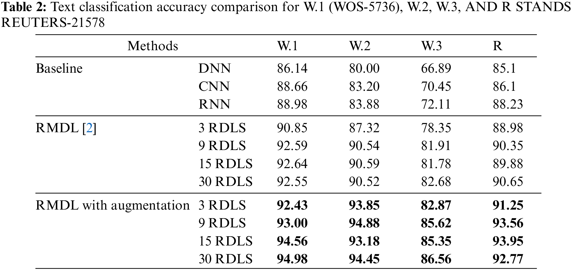
As Table 2 shows, RMDL with augmentation the accuracy has been enhanced comparing with the baselines. The empirical results in Table 2 are evaluated using four RMDL models (using 3, 9, 15, and 30 RDLs). The accuracy for Web of Science (WOS-5,736) is increased to 92.43, 93.00, 94.56 and 94.98 respectively. The accuracy for Web of Science (WOS-11,967), is improved to 93.85, 94.88, 93.18 and 94.45 respectively, and finally the accuracy for Web of Science (WOS-46,985) has improved to 82.87, 85.62, 85.35 and 86.56 correspondingly. The accuracy of Reuters-21578 is 91.25, 93.56, 93.95 and 92.77 respectively. As it is mentioned, the accuracy has been improved with all datasets.

Other datasets, such as the Large Movie Review Dataset (IMDB) and 20 NewsGroups, also have results. Table 3 shows how RMDL with augmentation improves accuracy for two ground truth datasets.

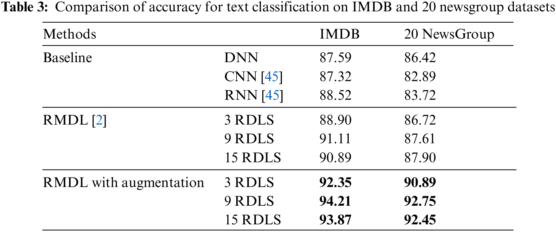
The accuracy of IMDB dataset is 92.35%, 94.21% and 93.87% respectively for 3, 9, and 15 RDLs, where the accuracy of DNN is 87.59%, CNN [45] is 87.32%, and RNN [45] is 88.52%. The accuracy of 20 NewsGroup dataset is 90.89%, 92.75% and 92.45% for 3, 9, and 15 random models respectively, where the accuracy of DNN is 86.42%, CNN [45] is 82.89%, and RNN [45] is 83.72%.

7  Conclusion and Discussion

In ML, to generalize findings of a classification task, we normally need to increase the training data amount, however, that causes the model to be overfitted and hence poorly performs on the testing set. In this work, an alternative mean of data augmentation problem using GANs has been introduced to overcome such a challenge. In particular, the proposed framework forces the convolutional architecture’s ability to learn low features for data capturing. By using these architectures, the data which is more meaningful and accurate can be collected. For classification, we used the RMDL model that solved the problem of choosing best technique in DL. The results show that combining RMDL with neural augmentation network provides improvements for classification for both images and text. The proposed approach has capability of improving model efficiency and accuracy and also can be used through a widespread variety of types of data.

Funding Statement: The researchers would like to thank the Deanship of Scientific Research, Qassim University for funding the publication of this project.

Conflicts of Interest: The authors declare that they have no conflicts of interest to report regarding the present study.

References

1. J. Chung, C. Gulcehre, K. Cho and Y. Bengio, “Empirical evaluation of gated recurrent neural networks on sequence modeling,” arXiv preprint arXiv:1412.3555, 2014. [Google Scholar]
2. K. Kowsari, M. Heidarysafa, D. E. Brown, K. J. Meimandi and L. E. Barnes, “Rmdl: Random multimodel deep learning for classification,” in Proc. of the 2nd Int. Conf. on Information System and Data Mining, NY, United States, pp. 19–28, 2018. [Google Scholar]
3. S. Robertson, “Understanding inverse document frequency: On theoretical arguments for IDF,” Journal of Documentation, vol. 60, no. 5, pp. 503–520, 2004. [Google Scholar]
4. B. Wang and D. Klabjan, “Regularization for unsupervised deep neural nets,” in Thirty-First AAAI Conf. on Artificial Intelligence, San Francisco, California, USA, pp. 2681–2687, 2017. [Google Scholar]
5. Y. Kubo, G. Tucker and S. Wiesler, “Compacting neural network classifiers via dropout training,” arXiv preprint arXiv:1611.06148, 2016. [Google Scholar]
6. Y. Gal and Z. Ghahramani, “A theoretically grounded application of dropout in recurrent neural networks,” in Proc. of the Advances in Neural Information Processing Systems, California, USA, pp. 1019–1027, 2016. [Google Scholar]
7. N. Srivastava, G. Hinton, A. Krizhevsky, I. Sutskever and R. Salakhutdinov, “Dropout: A simple way to prevent neural networks from overfitting,” The Journal of Machine Learning Research, vol. 15, no. 1, pp. 1929–1958, 2014. [Google Scholar]
8. S. Ioffe and C. Szegedy, “Batch normalization: Accelerating deep network training by reducing internal covariate shift,” in Int. Conf. on Machine Learning, PMLR, Lillie, France, pp. 448–456, 2015. [Google Scholar]
9. S. Xiang and H. Li, “On the effects of batch and weight normalization in generative adversarial networks,” arXiv preprint arXiv:1704.03971, 2017. [Google Scholar]
10. P. Y. Simard, D. Steinkras and J. C. Platt, “Best practices for convolutional neural networks applied to visual document analysis,” in Proc. of the Seventh Int. Conf. on Document Analysis and Recognition, Edinburgh, UK, pp. 958–962, 2003. [Google Scholar]
11. J. Lemley, S. Bazrafkan and P. Corcoran, “Smart augmentation learning an optimal data augmentation strategy,” IEEE Access, vol. 5, no.1, pp. 5858–5869, 2017. [Google Scholar]
12. J. Wang and L. Perez, “The effectiveness of data augmentation in image classification using deep learning,” Convolutional Neural Networks Vis. Recognit., vol. 11, no. 1, pp. 1–8, 2017. [Google Scholar]
13. S. C. Wong, A. Gatt, V. Stamatescu and M. D. McDonnell, “Understanding data augmentation for classification: When to warp?,” in 2016 Int. Conf. on Digital Image Computing: Techniques and Applications (DICTA), Gold Coast, Australia, IEEE, pp. 1–6, 2016. [Google Scholar]
14. C. Shorten and T. M. Khoshgoftaar, “A survey on Image Data Augmentation for Deep Learning,” Journal of Big Data, vol. 6, pp. 1–48, 2019. [Google Scholar]
15. G. Nagy, “Twenty years of document image analysis in pami,” IEEE Transactions on Pattern Analysis and Machine Intelligence, vol. 22, no. 1, pp. 38–62, 2000. [Google Scholar]
16. D. C. Cireşan, U. Meier, L. M. Gambardella and J. Schmidhuber, “Deep, big, simple neural nets for handwritten digit recognition,” Neural Computation, vol. 22, no. 12, pp. 3207–3220, 2010. [Google Scholar]
17. G. Loosli, S. Canu and L. Bottou, “Training invariant support vector machines using selective sampling,” Large Scale Kernel Machines, vol. 2, no. 1, pp. 301.320, 2007. [Google Scholar]
18. L. Perez and J. Wang, “The effectiveness of data augmentation in image classification using deep learning,” arXiv preprint arXiv:1712.04621, 2017. [Google Scholar]
19. E. D. Cubuk, B. Zoph, D. Mane, V. Vasudevan and Q. V. Le, “Autoaugment: Learning augmentation policies from data,” arXiv preprint arXiv:1805.09501, 2018. [Google Scholar]
20. S. Gurumurthy, R. Kiran Sarvadevabhatla and R. Venkatesh Babu, “Deligan: Generative adversarial networks for diverse and limited data,” in Proc. of the IEEE Conf. on Computer Vision and Pattern Recognition, Honolulu, HI, USA, pp. 166–174, 2017. [Google Scholar]
21. M. Marchesi, “Megapixel size image creation using generative adversarial networks,” arXiv preprint arXiv:1706.00082, 2017. [Google Scholar]
22. T. Salimans, I. Goodfellow, W. Zaremba, V. Cheung, A. Radford et al., “Improved techniques for training GANs,” Advances in Neural Information Processing Systems, vol. 29, no. 1, pp. 1–10, 2016. [Google Scholar]
23. L. Deng, “The mnist database of handwritten digit images for machine learning research [best of the web],” IEEE Signal Processing Magazine, vol. 29, no. 6, pp. 141–142, 2012. [Google Scholar]
24. A. Krizhevsky, V. Nair and G. Hinton, “The CIFAR-10 dataset,” 2014. [Online]. Available: http://www.cs.toronto.edu/kriz/cifar.Html. [Google Scholar]
25. X. Liang, Z. Hu, H. Zhang, C. Gan and E. P. Xing, “Recurrent topic-transition gan for visual paragraph generation,” in Proc. of the IEEE Int. Conf. on Computer Vision, Venice, Italy, pp. 3362–3371, 2017. [Google Scholar]
26. Y. Yu, Z. Gong, P. Zhong and J. Shan, “Unsupervised representation learning with deep convolutional neural network for remote sensing images,” in Int. Conf. on Image and Graphics, Shanghai, China, Springer, pp. 97–108, 2017. [Google Scholar]
27. Y. Li, T. Cohn and T. Baldwin, “Robust training under linguistic adversity,” in Proc. of the 15th Conf. of the European Chapter of the Association for Computational Linguistics, Short Papers, Valencia, Spain, vol. 2, pp. 21–27, 2017. [Google Scholar]
28. S. Kobayashi, “Contextual augmentation: Data augmentation by words with paradigmatic relations,” arXiv preprint arXiv:1805.06201, 2018. [Google Scholar]
29. T. Mikolov, I. Sutskever, K. Chen, G. S. Corrado and J. Dean, “Distributed representations of words and phrases and their compositionality,” Advances in Neural Information Processing Systems, vol. 26, no. 1, pp. 3111–3119, 2013. [Google Scholar]
30. S. Krishnan and M. Chen, “Identifying tweets with fake news,” in 2018 IEEE Int. Conf. on Information Reuse and Integration (IRI), Utah, USA, pp. 460–464, 2018. [Google Scholar]
31. Y. Sano, K. Yamaguchi and T. Mine, “Automatic classification of complaint reports about city park,” Information Engineering Express, vol. 1, no. 4, pp. 119–130, 2015. [Google Scholar]
32. M. Dundar, Q. Kou, B. Zhang, Y. He and B. Rajwa, “Simplicity of kmeans versus deepness of deep learning: A case of unsupervised feature learning with limited data,” in 2015 IEEE 14th Int. Conf. on Machine Learning and Applications (ICMLA), Miami, Florida, USA, pp. 883–888, 2015. [Google Scholar]
33. A. Das, D. Ganguly and U. Garain, “Named entity recognition with word embeddings and wikipedia categories for a low-resource language,” ACM Transactions on Asian and Low-Resource Language Information Processing (TALLIP), vol. 16, no. 3, pp. 1–19, 2017. [Google Scholar]
34. J. Pennington, R. Socher and C. D. Manning, “Glove: Global vectors for word representation,” in Proc. of the 2014 Conf. on Empirical Methods in Natural Language Processing (EMNLP), Doha, Qatar, pp. 1532–1543, 2014. [Google Scholar]
35. R. Rehurek and P. Sojka, “Software framework for topic modelling with large corpora,” in Proc. of the LREC 2010 Workshop on New Challenges for NLP Frameworks, Citeseer, Valetta, Malta, pp. 45–50, 2010. [Google Scholar]
36. V. Nair and G. E. Hinton, “Rectified linear units improve restricted boltzmann machines,” in Int. Conf. on Machine Learning, Haifa, Israel, pp. 807–814, 2010. [Google Scholar]
37. Y. Bengio, P. Simard and P. Frasconi, “Learning long-term dependencies with gradient descent is difficult,” IEEE Transactions on Neural Networks, vol. 5, no. 2, pp. 157–166, 1994. [Google Scholar]
38. J. Duchi, E. Hazan and Y. Singer, “Adaptive subgradient methods for online learning and stochastic optimization,” Journal of Machine Learning Research, vol. 12, no. 7, pp. 2121–2159, 2011. [Google Scholar]
39. M. D. Zeiler, “Adadelta: An adaptive learning rate method,” arXiv preprint arXiv:1212.5701, 2012. [Google Scholar]
40. K. Kowsari, D. E. Brown, M. Hei-darysafa, K. J. Meimandi, M. S. Gerber et al., Web of Science Dataset, 2018. https://doi.org/10.17632/9rw3vkcfy4.6. [Google Scholar]
41. F. Chollet, “Keras: Deep learning library for theano and tensorflow,” vol. 7, no. 8, pp. T1, 2015, URL: https://keras.io/k. [Google Scholar]
42. Y. Tang, “Deep learning using linear support vector machines,” arXiv preprint arXiv:1306.0239, 2013. [Google Scholar]
43. T. H. Chan, K. Jia, S. Gao, J. Lu, Z. Zeng et al., “Pcanet: A simple deep learning baseline for image classification?,” IEEE Transactions on Image Processing, vol. 24, no. 12, pp. 5017–5032, 2015. [Google Scholar]
44. Z. H. Zhou and J. Feng, “Deep forest: Towards an alternative to deep neural networks,” in Proc. of the Twenty-Sixth Int. Joint Conf. on Artificial Intelligence, Melbourne, Australia, pp. 3553–3559, 2017. [Google Scholar]
45. Z. Yang, D. Yang, C. Dyer, X. He, A. Smola et al., “Hierarchical attention networks for document classification,” in Proc. of the 2016 Conf. of the North American Chapter of the Association for Computational Linguistics: Human Language Technologies, San Diego, California, USA, pp. 1480–1489, 2016. [Google Scholar]
Cite This Article
Copyright © 2023 The Author(s). Published by Tech Science Press.
This work is licensed under a Creative Commons Attribution 4.0 International License , which permits unrestricted use, distribution, and reproduction in any medium, provided the original work is properly cited.
Downloads
Citation Tools