Federated Learning Based on Data Divergence and Differential Privacy in Financial Risk Control Research

1  Introduction

In the finance field, risk control has always been the most important link of the credit business of banks. Due to the increase in big data, machine learning has been widely applied to all aspects of life [1,2]. Namely, using big data to conduct risk control modeling has become the mainstream method in the finance field. This method mostly relies on the integration and sharing of loan data between banks. However, the increasingly strict domestic regulations on privacy protection have brought the problem of data silos, so a federal learning framework is necessary [3]. One research direction has been to reduce communication time and improve the risk control level of enterprises under the premise of ensuring data privacy [4]. However, there is a lack of effective means for non-id data [5]. Another research direction has been to optimize the convergence by optimizing the resource allocation of terminals, but this can cause problems of slow convergence speed and poor optimal solution accuracy [6,7]. To solve these problems, a classifier-based loan analysis model was proposed in [8], where a classifier based on min-max normalization (Min-Max) and k-nearest neighbor (KNN) method was used to predict loans. However, this method cannot guarantee data privacy. In reference [9], a system based on blockchain and intelligent contracts was developed to solve the problem of data center unreliability.

In the field of distributed machine learning, federated learning has been used to enable deep learning models to benefit from interrelated multi-node data [10,11]. However, it is necessary to explore more possibilities for federated learning, particularly the cooperation between multiple devices. Federal learning based on the SGD has been proven to have good performance in training deep networks, but the problem is that customer groups are different while their characteristics are basically the same. Therefore, this study selects horizontal federated learning [12,13]. In reference [14], a federated learning model with blockchain, which used the consensus mechanism of blockchain exchange learning, was presented; therefore, there was no need to process data. Currently, a federated averaging (FedAvg) algorithm [15], which can achieve high accuracy for iid data by model training on the MNIST and CIFAR-10 datasets, has been commonly used in the industry.

However, how to improve the convergence speed and accuracy of a model while ensuring data privacy has been the main challenge. In reference [16], a sparse ternary compression (STC) method, which uses a compression framework to improve federal learning under resource constraints, was proposed to overcome this challenge. The problems of model convergence and data heterogeneity in joint learning can be addressed by improving the FedAvg algorithm [17–19]. At present, federal learning has been applied to many fields, including health care, car driving, and communication. In addition, joint learning has been used to optimize the complexity of non-iid medical data [20,21].

Data privacy can be ensured by using differential privacy, but this method can affect model accuracy [22,23]. According to the analyses of the impact of differential privacy on machine learning-based models and application scenarios [24,25], there are two methods protects data privacy. The first method is to achieve local differential privacy while preserving graph accuracy, and this method protects data privacy through data splitting and combining [26,27]. Another method is to adopt a strategy that combines privacy-preserving data publishing with principal component analysis optimization (PPDP-PCAO) [28] to disturb local data and encrypt the reduced-dimensional data using homomorphic encryption to ensure data privacy.

The main contributions of this paper can be summarized as follows:

(1)   To handle scenes with non-iid data, a federated learning scheme based on global data sharing is proposed to overcome the problems of divergence explosion and slow convergence caused by data imbalance;

(2)   To ensure privacy in the data transmission process, a noise algorithm based on the commonly-used differential privacy is developed to improve model accuracy while ensuring data privacy by imposing different privacy budgets according to the contribution;

(3)   To overcome the problem of a certain difference between the fusion algorithm on the server side and the traditional asynchronous updating method, global and local models are assigned different weights according to the contribution degree algorithm based on the Bayesian theorem.

2  Related Work

In this section, an overview of recent studies on federated learning and differential privacy is provided, and a federated learning-based framework that uses differential privacy for local data sharing is proposed to address the risk control problem in the banking and credit industry so that each client can keep customer data confidential. The model is trained on the premise.

2.1 Federated Learning

The FedAvg algorithm is the basis of the federated learning-based algorithm. Recently, many studies have achieved certain improvements using the FedAvg algorithm. The FedAvg algorithm aims to increase the number of local updates while reducing the communication amount between a client and a server. In reference [29,30], it has been proven that the FedAvg algorithm converges under both iid and non-iid data sets, but the convergence speed is slower for non-iid data. Since each FedAvg client shares a fusion model, for non-independent same-distributed data, the gradient deviation of a locally-trained model is large, so the needs of each client cannot be met. This is demonstrated by the data comparison presented in Table 1. The global model has poor prediction performance on the client side due to data distortion [31].

The learning process is illustrated in Fig. 1.

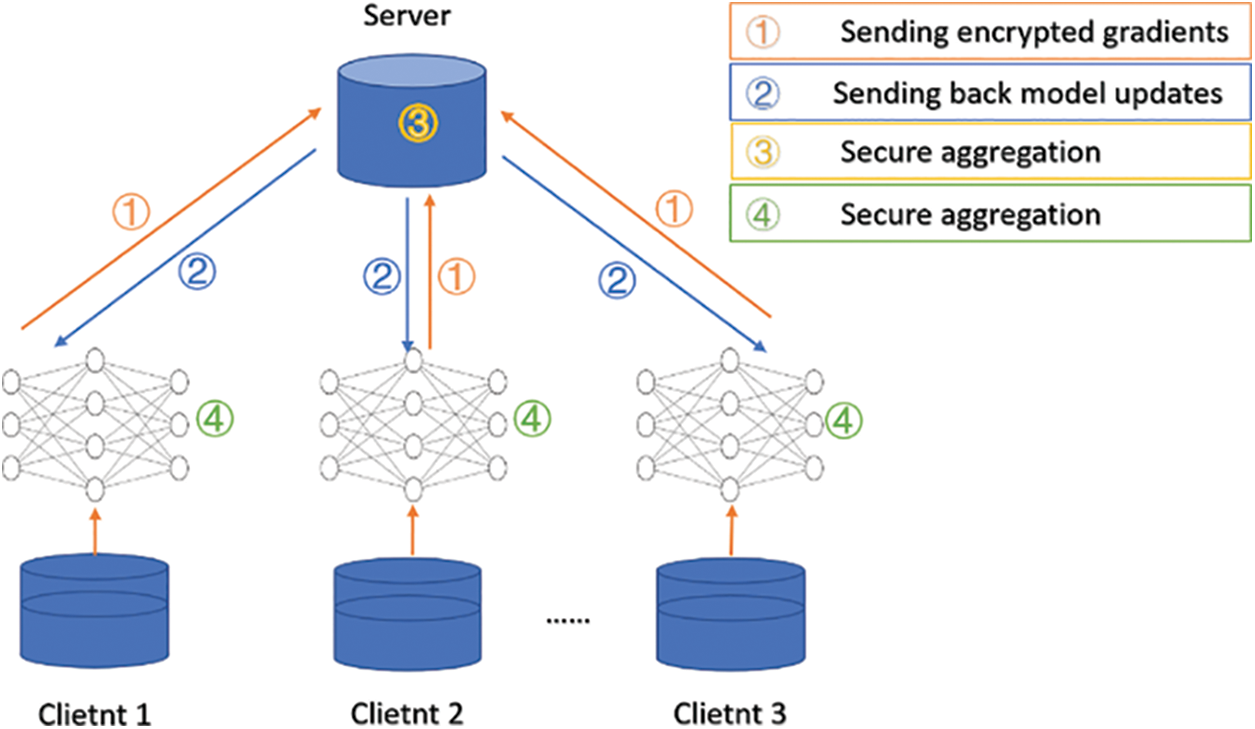
Figure 1: The architecture of the FedAvg algorithm

Step 1: A client downloads the original data model from server A;

Step 2: The client uses local database data to train the model, employs the mini-batch (small batch gradient descent) to minimize the local loss function of the model, and uploads the updated gradient to server A;

Step 3: Server A selects different clients according to contribution and uses average or weighted aggregate gradients to update the model parameters;

Step 4: The client downloads the updated model for personalization training, where the client cost function is given by

fj(ϕ)=12(ϕ−1ns∑i=1nsxj,i)2(1)

where ϕ is changed with the updated parameters of each client, and ϕj = ϕ + pj, and pj is the added Gaussian noise; training samples of each client are represented by xi,j.

The pseudo-code of the FedAvg algorithm is shown in Fig. 2.

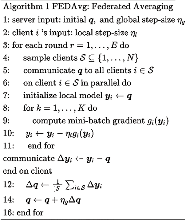
Figure 2: The pseudo-code of the FedAvg algorithm

Assume that there are N clients and each customer has a local dataset. During each iteration, a server sends the initial model to the client, which generates a small sample gradient descent according to the global state and local data. Generally, the optimization process for the d-dimensional data is as follows:

minw∈Rdf(q), wheref(q)=1n∑i=1nfi(q)(2)

Assuming that data of client I is denoted by Dk and n = |Dk|, the optimization goal can be reached for:

f(q)=∑k=1KnknFk(q), where Fk(q)=1nk∑i∈𝒫kfi(q)(3)

2.2 Differential Privacy Attack

The definition of differential privacy is as follows. For two datasets x, x′∈X with the Hamming distance of one, if x and x′ are adjacent datasets with only one element difference in input, then a randomization algorithm A: X → R for a subset S can be defined by:

x,x′∈D:Pr[f(x)∈S]≤eϵPr[f(x′)∈S]+δ(4)

Then, (ε, δ) differential privacy is satisfied.

One typical differential privacy attack principle is shown in Fig. 3.

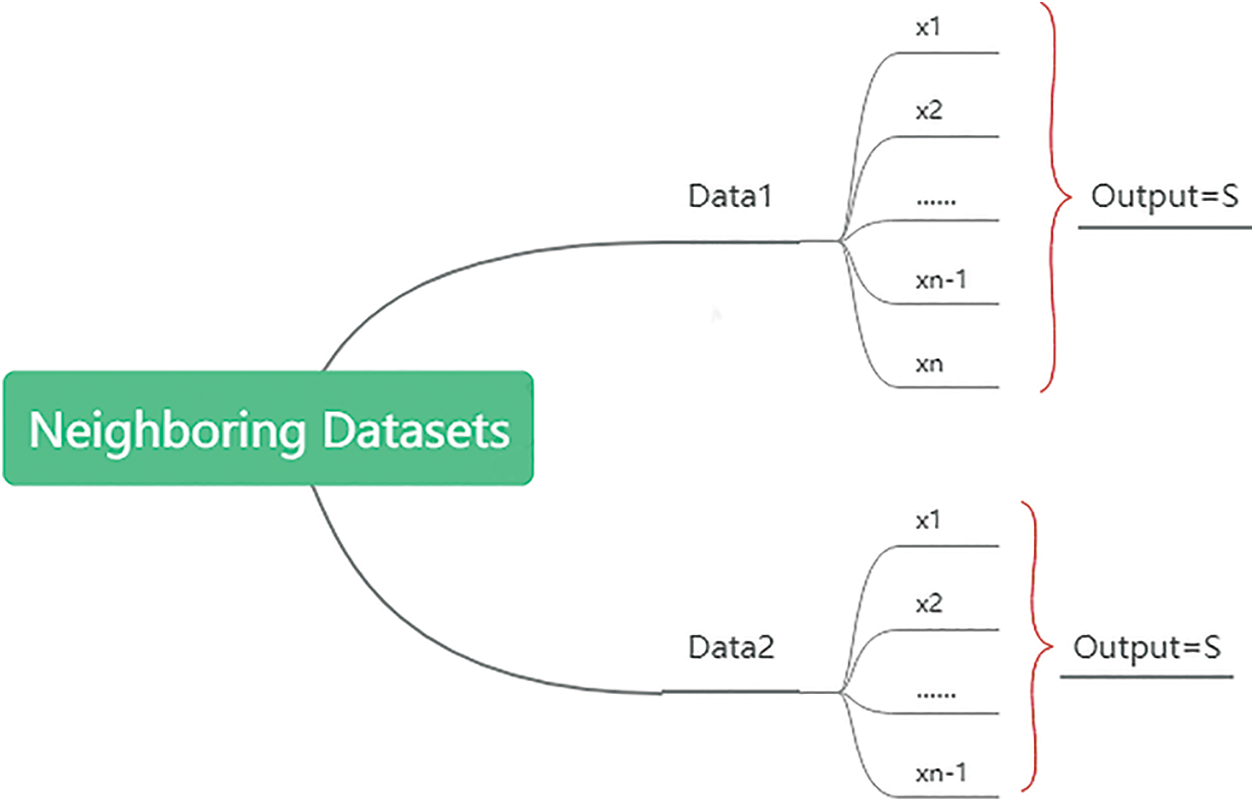
Figure 3: Obtaining dataset privacy using differential attacks

To deal with this attack, the basic idea of differential privacy is used to add the disturbance noise to data so that a single difference in the data does not generate a significant difference in the output results, thus preventing the loss of data availability. However, it is challenging to ensure the global model performs well on all customers’ local datasets. To reduce the performance degradation of joint learning caused by differential privacy, this study adopts optional differential privacy to solve this problem and enhances the performance of the improved model on the local dataset by 12% compared to the original model.

Definition 1: Differential privacy (ε, δ)

If x and x′ are adjacent datasets with only one-element difference in input, for two datasets x, x′ ∈D with a Hamming distance of one as input, and S as output, a randomization algorithm A: X→R, R for a subset S is defined as follows:

x,x′∈D:Pr[f(x)∈S]≤eϵPr[f(x′)∈S]+δ(5)

The differential privacy (ε, δ) is satisfied; the smaller the privacy budget ε is, the better the privacy protection will be, and the larger the added noise will be at the cost of the decline in data availability; δ is the probability of accidental disclosure that violates differential privacy under normal circumstances. As a relaxation term, it is usually defined as a small number, and in this paper, it is set to 0.02. The theorem has been proved in [22].

Definition 2: Sensitivity mechanism

Sensitivity represents the maximum variation range of two data sets x and x′ with a one-element difference. A query function f (·) is used to output the result, and it is defined by Eq. (6), where ||x||p represents the Lp-norm. The smaller the sensitivity is, the less noise needs to be added.

δf=maxX,X′∥f(X)−f(X′)∥1(6)

Definition 3: Noise mechanism

The common method of adding the noise is to randomize the query results without affecting the data output and adding the noise with a certain distribution. One of these methods is the Gaussian mechanism, where the noise with the Gaussian distribution is added to the query results; this method is suitable for numerical output. Another method is the exponential mechanism, where the exponential distribution is used to adjust the probability of query results, and this method is suitable for non-numerical output. This study introduces two variables: clipping and noise. Suppose that in each update, a client with a probability P is selected among M clients, and the clipping of the selected client is the norm. Then, after the average value of the update gradient values of the clients is calculated, the sum of the mean covariance and the Gaussian noise satisfying the distribution is taken as a variation range of difference privacy (ε, δ).

σ2I=z2(SPM)2I(7)

3  Formulation Methodology

3.1 System Architecture

The architecture of the data sharing-based FL algorithm (DSFL) includes two main layers, a data encryption layer and a data transmission layer, as shown in Fig. 4. The former is deployed locally on the client side, and the gradient is encrypted by adding the differential privacy noise after data alignment; meanwhile the latter consists of a server and M clients. The data encryption layer is used for gradient transmission between the central server and a client to update the federation model, and the data transmission layer is used for the central server to deploy a subset of the global data to a client to reduce the independence of local and global data distributions.

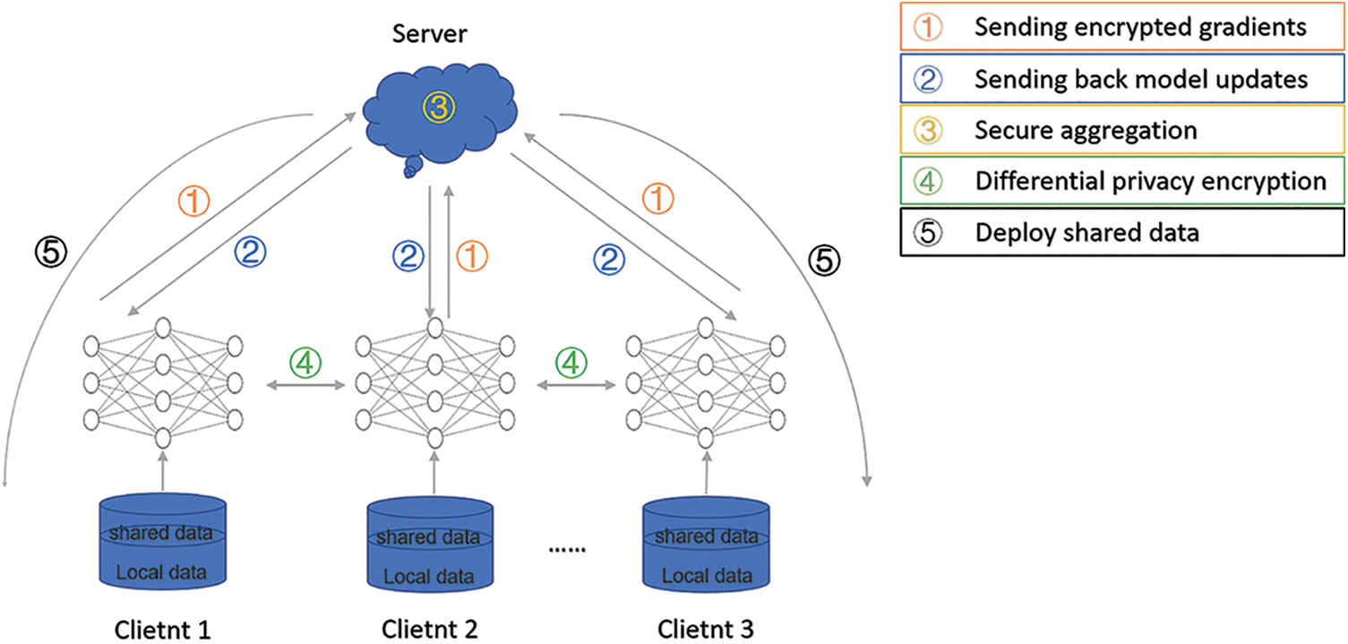
Figure 4: The DSFL architecture

In each update model iteration, m clients are selected from all clients by contribution, and the optimal gradient of the loss function J(f(qik−1,xj) is solved on the dataset consisting of the current client database and shared data.

∇g(qik−1;Di)=1|Di|∑j=1|Di|∂J(f(qik−1,xj),yj)∂qik−1(8)

Step 1: After a server receives a batch of clients, one part of desensitized data is sampled from all clients to form a global dataset S, and its subset is randomly deployed to the client according to proportion β;

Step 2: The client uses a small-batch SGD algorithm to update the gradient according to the local dataset Di and random subset Si of dataset S, and the loss function f(·) and step α to determine the local optimal gradient;

Step 3: The sampling is performed for different privacy to obtain the number of gradients n, and contribution degree function u(∇gj(qit−1;Di),Di) is used to obtain the gradient of the m largest contribution degrees and the smallest one to impose noise of different privacy budgets;

Step 4: After receiving the gradient uploaded by multiple clients, the server performs the weighted averaging according to the error function and updates the machine learning-based parameters;

Step 5: After downloading the latest model from the client, the server updates the local model with the global optimal gradient for the next training iteration.

3.2 Algorithm

Innovation 1: Data tilt in non-iid data

Based on the classical FedAvg algorithm proposed by Google, this study proposes a strategy to balance highly-skewed non-iid data using one part of the shared public data. The proposed method can be used to reduce data divergence between the client and server sides and improve the overall training accuracy of a model. The globally shared dataset is denoted by S, and it represents a uniformly distributed dataset that includes all categories of data. Dataset S is used to train the global initial model, and a random subset of S with a ratio of β is deployed to customers. Finally, the local and shared data are used jointly to train local models. The ratio β is given by:

β=∥S∥∥N∥×100% (9)

Innovation 2: Shared data collection and client update

Each client is defined according to its local data distribution {xit,j,yit,j}j=1m; select a random distribution dataset with a data ratio β and all local classes for updating S.

A client i receives the initial model q0 and a random subset of the globally shared dataset S and uses GSD (f(·), B + S, α) to update the local gradient because function f is strongly convex. The client can update a local gradient to make it close to the global loss minimum, with a time complexity O(log1/α).

fj(ϕ)=12(ϕ−1ns∑i=1nsxj,i)2(10)

Innovation 3: Server update gradient

Nodes are assigned weights according to the contribution of the global and local models.

After the updated gradient qt of a client is sent to a server, the model weight distribution of the global client is initialized. Next, the client gradient weight distribution is updated according to the error function, and finally, a weighted average classifier model is obtained. The client model weight update process is as follows. Weight αt of this model should be set such that αtqt minimizes the exponential loss function.

ιexp(αtqt|𝒟t)=Ex∼𝒟t[e−f(x)αtqt(x)]=Ex∼𝒟t[e−αtI(f(x)=qt(x))+eαtI(f(x)≠qt(x))]=e−αtPx∼𝒟t(f(x)=qt(x))+eαtPx∼𝒟t(f(x)≠qt(x))=e−αt(1−ϵt)+eαtϵt(11)

where the exponential loss function is derived so that it equals zero.

∂ιexp⁡(αtqt|𝒟t)∂αt=−e−αt(1−ϵt)+eαtϵt(12)

Further, αt is the weight update coefficient of the local gradient function, and it is given by:

αt=12ln⁡(1−ϵtϵt)(13)

Innovation 4: Data privacy concerns

This paper proposes using decentralized differential privacy. According to the contribution difference between the gradient values of different dimensions of the local model and the contribution function, different privacy budgets are used to add the noise. When a local gradient is calculated, data samples are divided into a small batch of data Di, which corresponds to the local gradient model obtained by the SGD algorithm, where J(f(qik−1,xj),yj) is the loss function.

The gradient is calculated by:

∇g(qik−1;Di)=1|Di|∑j=1|Di|∂J(f(qik−1,xj),yj)∂qik−1(14)

Client P updates the gradient using the local model as follows:

qik=qik−1−ηi∇g(qik−1;Di)(15)

Based on the small batch of data Di, the local gradient model ∇gj(qit−1;Di) is obtained, and the availability of gradients of different dimensions is calculated using the contribution function R as follows:

u(∇gj(qit−1;Di),Di)=|∇gj(qit−1;Di)|,j=1,2,…,n(16)

Then, the exponential mechanism is used to sample n model gradient values to obtain the total privacy budget εi as follows:

Pr[∇gl∈∇g(qit−1;Di)]∝exp⁡(εiu(∇gl,Di)2nΔu),l=1,2,…,n(17)

The higher the contribution degree of a gradient value of the local model is, the greater its chance to be selected will be. The Laplacian noise with a privacy budget of ε2 is added to the gradient with the largest contribution value for the first m; the Laplacian noise with a privacy budget of ε3 is added to the last (n – m) gradients.

∇g^l(qit−1;Di)=∇gl(qit−1;Di)+Lapl(Δqεi)(18)

When L is in the range of [1, m], i = 2 is the Laplacian noise with a privacy budget of ε2, and when L is in the range of [m, n], then i = 3, and the local optimal gradient model is generated after many local iterations. After the weighted average is obtained, it is uploaded to the server to update the model.

4  Experimental Results

4.1 Dataset Definition

Two public datasets 1, Loan (https://www.kaggle.com/itsmesunil/bank-loanmodelling) and Abank credit department (BANK data set), were used to classify personal loan behavior.

After obtaining a total of 12,047 samples with a total of 31 user features, the problem of missing dimensions in the samples was addressed as follows. Data scaling and data discretization were adopted for digital fields. According to the width, frequency, and clustering features, the features such as age were mapped to the interval, and the interval id instead of the specific value was used to perform the numerical mapping.

The string-type data were used for hot coding. Data of different structures were unified and converted into a Hive table for subsequent calculation. Considering the missing degree of samples, features with a missing degree of more than 50% were discarded. As shown in Fig. 5, Based on the principle of IV statistics, feature vectors were selected continuously by boxes. Finally, the remaining 10 features were trained.

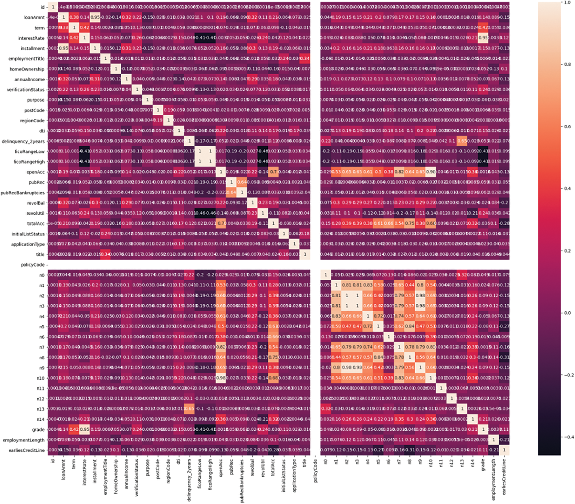
Figure 5: The correlation between features obtained based on the covariance matrix

The data were divided into training and test sets according to the proportion of 8:2. The training set was divided between 12 clients on average, and the training samples were divided into 10 classes. Next, 1,000 data samples, including 10 classes, were selected to form a shared dataset as a global shared data subset S; the number of clients was set to five. The training set was randomly and unequally deployed at the client as a local database.

Two commonly-used indicators were selected to evaluate model quality. The canonical term coefficients of accuracy and loss were set to 0.0005, and the step size was set to 0.001.

4.2 Comparison with FedAvg Algorithm

First, experiments with the proposed method were conducted on the iid and non-iid datasets. The FedAvg algorithm was used as a baseline, and experiments were divided into three groups. The DSFL algorithm was performed on the iid dataset, and the FedAvg and DSFL algorithms were applied to the other two groups of non-IID data. Each client’s local dataset in the iid data was randomly, uniformly distributed across all classes. The non-iid data were arranged according to the class labels into 20 partitions, making the client receive data from only a certain number of classes. The other parameters were set as follows. The number of clients was N, the number of training epochs was E, the local calendar was set to one, and the learning rate of the client was α = 0.02.

As shown in Fig. 6, the accuracy of the DSFL algorithm reached 87.6% after being stabilized on the dataset with the balanced distribution, while for the second type of dataset with data distortion, the non-iid dataset 1, the DSFL algorithm had better performance than on the second non-iid dataset. After stabilization, the convergence round number was decreased by six, and the accuracy rate increased by 7%.

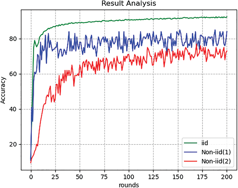
Figure 6: The accuracy result comparison of the algorithms on the iid dataset and two non-iid datasets

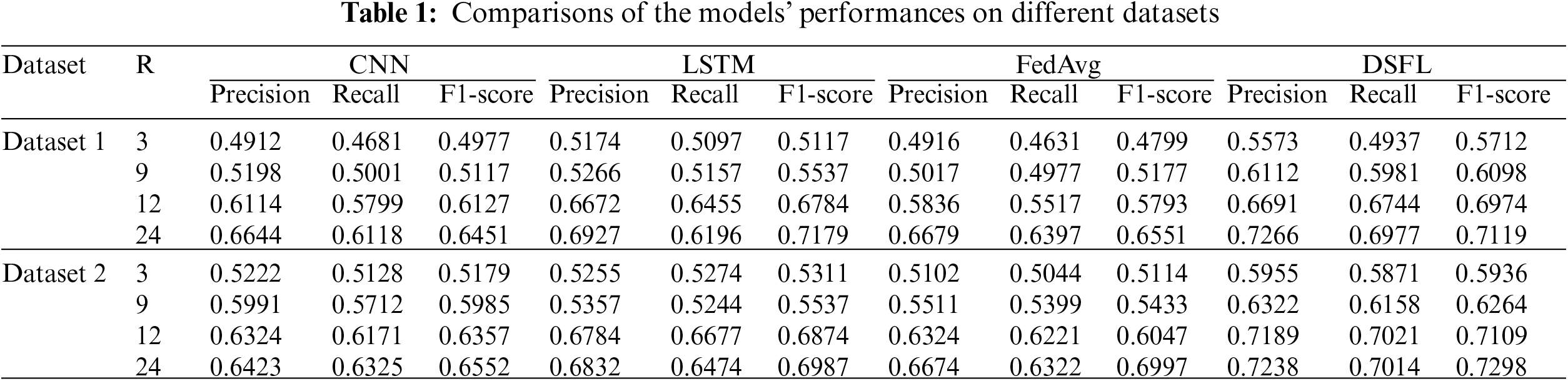
To verify the effectiveness of the proposed DSFL method, comparative experiments were conducted with several mainstream models, including the CNN model (Taheri et al. 2021), LSTM model (Yuwei Sun et al. 2021), and classic FedAvg model, with the same simulation configuration on datasets 1 and 2. The experimental results are shown in Table 1.

As shown in Table 1, for the loan prediction task, the proposed algorithm had a significant advantage in accuracy compared to the CNN, LSTM, and FedAvg models. There were 24 training rounds. The precision, recall, and F1-score of DSFL were 0.7266 model, 0.6977, and 0.7119, respectively. The FedAvg model had the precision, recall, and F1-score values of 0.6679, 0.6397, and 0.6551, respectively. Although the accuracy of the subsequent training performed according to the different privacy budgets was improved, the proposed algorithm had a good performance because using the shared data could more effectively solve the problem of horizontal federation learning data imbalance. Compared with the local models CNN and LSTM, the FedAvg algorithm sacrificed the accuracy to a certain extent compared to the LSTM and CNN algorithms in the process of passing the gradient to ensure data privacy. The DSFL could significantly reduce this impact by using the noise of different privacy budgets in data privacy tasks. The DSFL had a greater advantage.

Next, the following two points were verified in the experiment:

(1) The influence of privacy budget on accuracy and loss function;

(2) The influence of shared data on model accuracy.

4.3 Privacy Budget Effect on Model Accuracy and Loss Function

A feedforward neural network (FFNN) was used to train the model; the hidden layer included three layers and had N input features; the number of neurons was N or 2N, and the N output layer consisted of a single neuron. The mini-batch SGD algorithm was employed for local gradient optimization, using the cross-entropy loss function as a loss function L=−[ylogy^+(1−y)log⁡(1−y^)]. The learning rate of local learning µ was set to 0.01, and the local mini-batch data size D was set to 100.

As shown in Fig. 7, adding the noise reduced the accuracy to a certain extent. According to the Laplacian noise addition formula, the smaller the privacy budget was, the greater the impact of the added noise on the result was. The protection degree was good, and the convergence occurred after approximately 80 epochs. The loss was fixed at nearly 0.5. In this study, an adjustable privacy mechanism was used to achieve a balance between privacy and model availability, providing a certain availability, which is proven below.

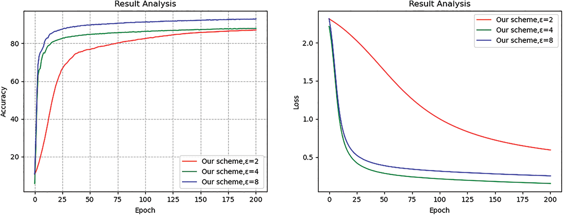
Figure 7: Impact of different privacy budgets on model accuracy and loss

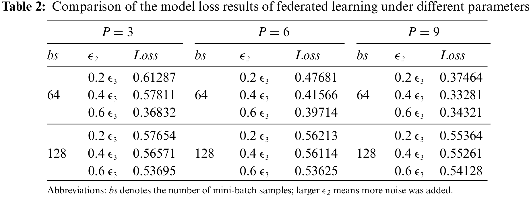
As shown in Table 2, When the mini-batch data size was 64, the accuracy was higher than that when the mini-batch data size was 128. The results indicated that the accuracy of the global model was improved, and the convergence speed of the model was increased at the cost of training time. When ϵ1 and ϵ3 were unchanged, and the proportion of ϵ2 was large, the model accuracy was improved. It is worth noting that the accuracy of the global model differed at different values of ϵ2 (0.25/0.5). Namely, there were obvious changes in accuracy, and the results demonstrated that the adopted differential privacy could provide higher balance accuracy and better privacy.

4.4 Shared Data Effect on Model Accuracy

The divergence of a client and a server with the same initialization was calculated by Eq. (20) Confirmation of changes, and it was affected by the learning rate, the number of synchronizations, and the gradient magnitude. The accuracy decreased with the divergence degree (DD), and the DD could be effectively reduced by global data sharing.

DD=∑i=1C||q(k)(y=i)−q(y=i)||(20)

The proposed method did not change the client dataset but sent a small portion of shared data with uniform data distribution to the server contributed by all clients, which resulted in a random data distribution on the server. After the client model was initialized, it was expected to reduce the DD and improve the accuracy of the global model.

β=||S||||N||×100% (21)

The training data were divided into two parts, one was the client dataset D, and the other was dataset S. This experiment considered more extreme and distorted class 1 non-iid data of the two types of non-iid datasets; namely, the dataset contained only one class. In the data initialization phase, the server deployed a partial subset α of S to each client for initialization, and the client used the two parts of data to train the local model. Then, Eq. (1) was used to evaluate the effect of data scale β of G and S on the model accuracy, and Eq. (2) was used to analyze the effect of the partial subset of S on the model accuracy.

The influence of β in 0%–25% on the model’s accuracy is presented in Fig. 8a, where it can be seen that after 400 training epochs, with the continuous increase in β, the accuracy reached the value of 78.42%. Even when the lower 10% was used, an accuracy rate of 72.86% could be achieved. Under the same settings, the accuracy rate without using the shared data was only 38%. Because the accuracy rate was flattened at only 25%, it was not required to deploy too much data to the client. With the increase in β, the DD first decreased and then stabilized at approximately 25%.

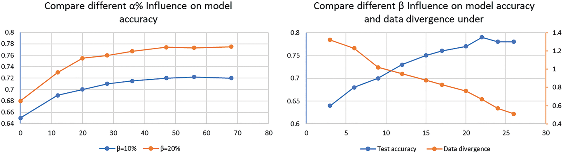
Figure 8: The influence comparison of α and β on data accuracy

The same changing trend can be observed in Fig. 8b. The accuracy of the model first increased rapidly and then stabilized in the range from 76% to 78%. Therefore, based on the experimental results, the amount of data deployed to a client could be reduced. For instance, when 10% of client data were used as the global shared data and α was set to 40%, only 5% of the data was needed to improve the overall model accuracy by 22%.

Consequently, the proposed shared data strategy provided a better solution to the considered federated learning problem, but the error was too large on the non-iid data.

5  Conclusions and Future Work

For data with strong privacy and large distribution differences, this paper uses the data divergence degree and adopts the federated learning algorithm with gradient fusion and Gaussian noise addition, which has a slight influence on model accuracy but can provide good robustness against differential attacks. Differences in the data distribution between clients are quantified, and the training accuracy of the model is improved and verified by sharing 5% of the data.

In future work, the proposed method could be improved to handle highly private data, such as lung CT photos of patients with COVID-19 infection, for medical disease prediction, and the adopted technology could be improved using effective methods and clustering algorithms for clients. In addition, clustering committees could be used to assign each client a different contribution degree, and more complex reinforcement learning-based models could be employed to reduce the number of clients participating in training without reducing model accuracy.

Funding Statement: This research was supported by the National Natural Science Foundation (NSFC), China, under the National Natural Science Foundation Youth Fund program (J. Hao, No. 62101275).

Conflicts of Interest: The authors declare that they have no conflicts of interest to report regarding the present study.

References

1. S. Mussiraliyeva, B. Omarov, P. Yoo and M. Bolatbek, “Applying machine learning techniques for religious extremism detection on online user contents,” Computers, Materials & Continua, vol. 70, no. 1, pp. 915–934, 2022. [Google Scholar]
2. M. Ragab, H. A. Abdushkour, A. F. Nahhas and W. H. Aljedaibi, “Deer hunting optimization with deep learning model for lung cancer classification,” Computers, Materials & Continua, vol. 73, no. 1, pp. 533–546, 2022. [Google Scholar]
3. R. Fantacci and B. Picano, “Federated learning framework for mobile edge computing networks,” CAAI Transactions on Intelligence Technology, vol. 7, no. 3, pp. 2322–2468, (Online2020. [Google Scholar]
4. J. Jiang and L. Hu, “Decentralised federated learning with adaptive partial gradient aggregation,” CAAI Transactions on Intelligence Technology, vol. 5, no. 3, pp. 230–236, 2020. [Google Scholar]
5. Y. R. Chen, J. S. Leu, S. A. Huang, J. T. Wang and J. I. Takada, “Predicting default risk on peer-to-peer lending imbalanced datasets,” IEEE Access, vol. 9, no. 22, pp. 73103–73109, 2021. [Google Scholar]
6. C. Shen, J. Xu, S. Zheng and X. Chen, “Resource rationing for wireless federated learning: Concept, benefits, and challenges,” IEEE Communications Magazine, vol. 59, no. 5, pp. 82–87, 2021. [Google Scholar]
7. S. Wang, T. Tuor and T. Salonidis, “Adaptive federated learning in resource constrained edge computing systems,” IEEE Journal on Selected Areas in Communications, vol. 37, no. 6, pp. 1205–1221, 2019. [Google Scholar]
8. G. Arutjothi and C. Senthamarai, “Prediction of loan status in commercial bank using machine learning classifier,” in 2017 Int. Conf. on Intelligent Sustainable Systems (ICISS), Palladam, India, pp. 416–419, 2017. [Google Scholar]
9. Y. Li, Y. Zhou, Y. Liu and R. N. Nortey, “Design of decentralized personal loaning platform based on blockchain,” in Int. Conf. on Electronic Information Technology and Computer Engineering (EITCE), Xiamen, China, pp. 22–31, 2019. [Google Scholar]
10. D. Rothchild, A. Panda, E. Ullah, N. Ivkin, I. Stoica et al., “FetchSGD: Communication-efficient federated learning with sketching,” in Proc. of the 37th Int. Conf. on Machine Learning, virtual Event, vol. 119, pp. 8253–8265, 2020. [Google Scholar]
11. T. Tieleman and G. Hinton, “Divide the gradient by a running average of its recent magnitude. cours-era: Neural networks for machine learning,” in Conf. and Workshop on Neural Information Processing Systems, Lake Tahoe, Nevada, USA, pp. 26–31, 2012. [Google Scholar]
12. J. Zhang, Y. Wu and R. Pan, “Auction-based ex-post-payment incentive mechanism design for horizontal federated learning with reputation and contribution measurement,” arXiv: 2201.02410, 2022. [Online]. Available: https://arxiv.org/abs/2201.02410. [Google Scholar]
13. Q. Li, X. Wei and H. Lin, “Inspecting the running process of horizontal federated learning via visual analytics,” IEEE Transactions on Visualization and Computer Graphics, vol. 27, no. 47, pp. 1, 2021. [Google Scholar]
14. H. Kim, J. Park, M. Bennis and S. Kim, “Blockchained on-device federated learning,” IEEE Communications Letters, vol. 24, no. 6, pp. 1279–1283, 2020. [Google Scholar]
15. H. B. McMahan, E. Moore, D. Ramage, S. Hampson and B. A. Arcas, “Communication efficient learning of deep networks from decentralized data,” in Int. Conf. on Artificial Intelligence and Statistics, Lauderdale, FL, USA, pp. 1273–1282, 2017. [Google Scholar]
16. F. Sattler, S. Wiedemann, K. R. Müller and W. Samek, “Robust and communication-efficient federated learning from non-iid data,” IEEE Transactions on Neural Networks and Learning Systems, vol. 31, no. 9, pp. 3400–3413, 2020. [Google Scholar]
17. B. Lim, N. C. Luong, D. T. Hoang and Y. Jiao, “Federated learning in mobile edge networks: A comprehensive survey,” IEEE Communications Surveys & Tutorials, vol. 22, no. 3, pp. 2031–2063, 2020. [Google Scholar]
18. S. Zheng and X. Unequal, “Unequal error protection transmission for federated learning,” IET Communications, vol. 16, no. 10, pp. 1106–1118, 2022. [Google Scholar]
19. T. Li, A. K. Sahu, M. Zaheerand and M. Sanjabi, “Federated optimization in heterogeneous networks,” Parts of Proceedings of Machine Learning and Systems, vol. 41, no. 13, pp. 421–441, 2020. [Google Scholar]
20. L. Huang, Y. Yin, Z. Fu, S. Zhang, H. Deng et al., “LoAd-boost: Loss-based adaboost federated machine learning with reduced computational complexity on IID and non-IID intensive care data,” PLoS One, vol. 17, no. 26, pp. 1–16, 2020. [Google Scholar]
21. F. Ongati and E. L. Muchemi, “Big data intelligence using distributed deep neural networks,” arXiv: 1909.02873, 2019. [Online]. Available: https://arxiv.org/abs/1909.02873. [Google Scholar]
22. J. Zhu and M. Blaschko, “Differentially private SGD with sparse gradients,” arXiv: 2112.00845, 2021. [Online]. Available: https://arxiv.org/abs/2112.00845. [Google Scholar]
23. W. Xiang, “An adaptive federated learning scheme with differential privacy preserving,” Future Generation Computer Systems (FGCS), vol. 127, no. 12, pp. 362–372, 2022. [Google Scholar]
24. B. Li and C. Wang, “A comprehensive survey on local differential privacy,” Security and Communication Networks, vol. 42, no. 17, pp. 988–1017, 2020. [Google Scholar]
25. S. dano and T. Murakami, “Degree-preserving randomized response for graph neural networks under local differential privacy,” arXiv: 2202.10209, 2022. [Online]. Available: https://arxiv.org/abs/2202.10209. [Google Scholar]
26. J. Ribes-González and S. Ricci, “Privacy-preserving data splitting: A combinatorial approach,” Designs, Codes and Cryptography, vol. 89, no. 2, pp. 1735–1756, 2021. [Google Scholar]
27. M. L. Erani and D. Croce, “Rings for privacy: An architecture for large scale privacy-preserving data mining,” IEEE Transactions on Parallel and Distributed Systems, vol. 32, no. 6, pp. 1340–1352, 2021. [Google Scholar]
28. W. Li, X. Zhang and X. Li, “An efficient high-dimensional data releasing method with differential privacy protection,” IEEE Access, vol. 7, no. 16, pp. 176429–176437, 2019. [Google Scholar]
29. T. Su, H. Qi and M. Brown, “Measuring the effects of non-identical data distribution for federated visual classification,” arXiv: 1909.06335, 2019. [Online]. Available: https://arxiv.org/abs/1909.06335. [Google Scholar]
30. Y. Hao, M. Li and Lai, “Federated learning with Non-IID data,” arXiv: 1806.00582, 2022. [Online]. Available: https://arxiv.org/abs/1806.00582. [Google Scholar]
31. D. Verma, G. White and S. White, “Approaches to address the data skew problem in federated learning,” Proceedings of SPIE (Proceedings. SPIE-The International Society for Optical Engineering), vol. 11006, no. 7, pp. 110061I–16, 2019. [Google Scholar]
Cite This Article
Copyright © 2023 The Author(s). Published by Tech Science Press.
This work is licensed under a Creative Commons Attribution 4.0 International License , which permits unrestricted use, distribution, and reproduction in any medium, provided the original work is properly cited.
Downloads
Citation Tools