A Novel Contour Tracing Algorithm for Object Shape Reconstruction Using Parametric Curves

1  Introduction

Computer graphics and geometric modeling are based on curves [1,2]. The theory of curves constitutes a very comprehensive field of study in geometry and is widely used in different applications of mathematics, physics, differential equations, and engineering [3]. In addition, curves are widely used in modern image processing and computer vision algorithms [4]. Among these algorithms, those related to defining the object shape use the edges in the image. An edge, which is a part of a boundary, corresponds to points in an image where the intensity value changes significantly from one pixel to the neighbor pixel. Identifying the boundary of an object is a crucial step toward a thorough understanding and analysis of the object. Edges not only carry structural information about the object but also help to significantly reduce the image memory capacity [5–7]. Therefore, in image processing applications, it is important to develop algorithms that find the edge positions of an object in an image with high accuracy and speed. The counter tracing algorithm is one of the many developed methods for this purpose. Most contour tracing algorithms run on binary images. These algorithms include three main steps. The first step is finding the starting point of the tracing. The second step is determining the next direction of the tracing movement. The final step is to terminate the tracing if the stopping criteria occur. There are very few contour tracing methods in the literature. The most widely used traditional counter-tracing algorithms are the worm-following method, raster scan method, and T algorithm [8]. Common problems with these algorithms are that tracing the same counter in some areas causes unnecessary looping, and incomplete tracing can occur if there are multiple discontinuities at the object boundary. Because of these difficulties, only findContours and Moore-Neighbor Tracing algorithms in the OpenCV library have had the chance to become commercially widespread. In order to reconstruct the object shape with parametric curves, the findContours algorithm cannot be used because the points belonging to the outer boundaries of the object must be obtained sequentially. In addition, this algorithm also finds the edge points of structures such as patterns in the object area, which are not required for the reconstruction of the object shape with parametric curves. The Moore algorithm, on the other hand, cannot complete the contours, especially if there are discontinuities in the object boundary lines. Therefore, this study proposes a new tracing algorithm to reveal sequential contour points that parametric curves can use.

Reconstruction of an object in an image, with a different translation, scaling, or orientation can be performed using parametric curves such as Bézier and B-splines. For this, curve equations need to be revealed using the set of points representing the object’s shape. The points that will be used to define the parametric curve that reconstructs the object shape must be sequential. Traditional edge detection algorithms find object edges, but the resulting points are often not sequential. In this study, a novel contour tracing algorithm has been developed that sequentially obtains the object boundary points. The proposed algorithm, unlike the methods in the literature, is implemented using a filter containing weights and a circle surrounding the object in the image. The contributions of this study to the literature can be summarized as follows:

•   Since the control points used in parametric curves such as Bézier and B-splines must be sequential, a new contour tracing algorithm has been developed that sequentially obtains the object boundary points to reconstruct the object shape,

•   The proposed algorithm introduces a new approach by using a filter that generates unique values for the algorithm to determine the boundary points and the next direction of movement,

•   For tracing an entire object boundary consisting of more than one open curve, a circle is used that surrounds the object, providing a starting point for each segment,

•   Bézier and B-spline curves are defined using the sequential outer boundary points obtained with the developed contour tracing algorithm,

•   The performances of Bézier and B-spline curves in reconstructing the object shape with a different translation, scaling, or orientation and the superiority of B-spline have been experimentally demonstrated,

•   It has been shown that the deformations on the outer boundary of the object in the image due to different reasons can be eliminated using parametric curves such as Bézier and B-splines.

•   Our proposed algorithm obtained better tracing results than Moore’s method while close to the findContours algorithm.

2  Parametric Curves

Parametric representations can be considered as the movement of a point in a certain time interval. Therefore, in the definition of such a curve, the curve is a set of positions based on the continuous time variable. Parametric curves do not require much memory as well as provide convenience in manipulating the surface shapes. For these reasons, parametric curves and surfaces are highly preferred in surface modeling, especially in the field of Computer-Aided Design (CAD) and Computer Aided Manufacturing (CAM) [9]. There are many different definitions of curves and surfaces for parametric representations. In this study, Bézier and B-spline curves, which are widely used in computer science, were used.

2.1 Bézier Curves

Bézier curves were first developed by Paul de Faget de Casteljau and Pierre Bézier to obtain smooth surfaces suitable for modeling automobiles [10,11]. The most comprehensive information on Bézier curves and geometries is available in Gerald Farin’s book “Curves and Surfaces for CAGD” [2]. Bézier curves have a wide range of uses, such as computer graphics, CAD, CAM, font design, vector drawing and 3D modeling [12]. In general, the Bézier curve is directly related to the vertices of the polygon that will define the curve shape. Only the first and last vertices of the polygon are on the curve, while the other vertices contribute to determining the degree of the curve and defining its shape. The degree or size of a Bézier curve is determined by the number of control points that form that curve. For example, a line is created from two control points, while a quadratic curve is created with three. More precisely, n + 1 control points are required to construct a Bézier curve of degree n. The Bézier curve with any degree n is expressed as in Eq. (1):

P(t)=∑i=0nPin!i!(n−i)!ti(1−t)n−i(1)

where Pi is the control point, and t is the time in [0, 1] intervals. For example, a Bézier curve with third-degree (n = 3) is defined by 4 (n + 1) control points (P0, P1, P2, and P3). Substituting the value of 3 for n in Eq. (1) yields the commonly used cubic curve Eq. (2) [13], and samples of cubic Bézier curves are given in Fig. 1 [14].

P(t)=(1−t)3P0+3(1−t)2tP1+3(1−t)t2P2+t3P3(2)

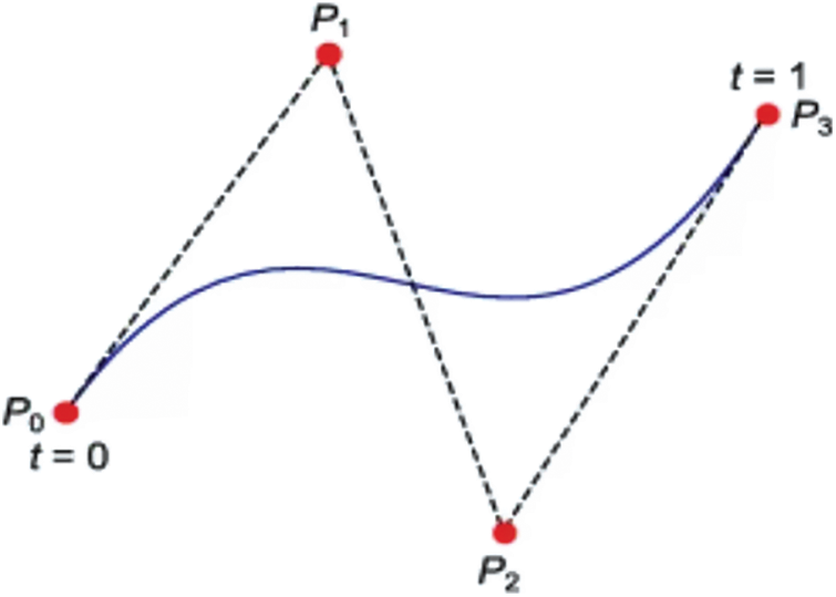
Figure 1: Sample for cubic Bézier curve with control points

2.2 B-spline Curves

The B-spline proposal for curves and surfaces was first introduced by Isaac Jacob Schoenberg and developed by Richard Riesenfeld, pioneering its use in CAD and CAM [15–18]. B-spline curves were developed to solve some of the problems encountered in the Bézier [19]. B-spline generally does not consist of a single segment like Bézier. B-spline consists of at least one or more polynomial segments. Therefore, the Bézier curve provides only global control, while the B-spline curve also allows local control. Since the basis functions used by B-spline are equal to zero except for their respective segments, the shape of the curve depends only on the corresponding control points. In other words, when the position of any control point in the Bézier curve is changed, the entire curve is affected by this change, while only a certain part of the curve is affected in the B-spline curve [20,21]. Despite this advantage, the B spline curves are more challenging and complex to program than the Bézier curves. A B-spline curve sample consisting of two polynomial segments is given in Fig. 2.

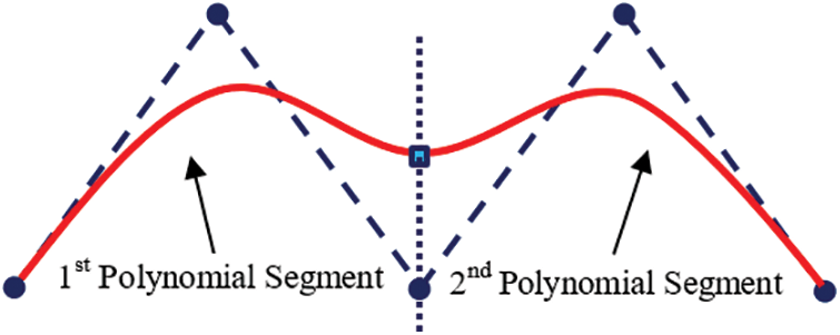
Figure 2: A B-spline curve with two segments

The appropriate order (k) value should be selected in the interval [2, n + 1] to form the desired shape of the B-spline curve defined by n + 1 control points. With the selected k value, both the number of segments (n − k + 2) and the degree of the curve (k − 1) are determined. Fig. 3 shows the effect of the selected k values on the shape of a B-spline curve [22]. As can be seen from the figure, if a small k value is selected, the number of segments increases, and the curve approaches the control points. If the rank is chosen as the lowest value (k = 2), the curve passes through all control points, and each segment consists of a line connecting two control points. If the number and order of control points defining the B-spline curve are equal (k = n + 1), the curve consists of a single segment, which is also a Bézier curve.

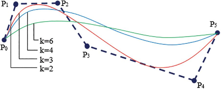
Figure 3: Effect of k value on B-spline curve shape

The mathematical representation of B-spline curves is given in Eq. (3) [23].

P(u)=∑i=0nPiNi,k(u)(3)

B-spline curves are calculated using Cox-de Boor functions. Ni,k(u) in Eq. (4) is the basis function of order k. In order to calculate this function, it is necessary to recursively calculate the basis functions for all orders less than k, including the first order [23].

Ni,k(u)=u−titi+k−1−tiNi,k−1(u)+ti+k−uti+k−ti+1Ni+1,k−1(u)(4)

Eq. (5) is valid for all k = 1 basis functions.

Ni,1(u)={1,  ti≤u<ti+10,  otherwise(5)

3  Contour Tracing Algorithm

In order to define an object shape with a curve equation, the points belonging to the outer boundary must be obtained sequentially depending on the neighborhood relations. Widely used edge detection methods such as Canny, Sobel, and Prewitt [24] do not offer the option of detecting the outer boundary points in a sequential manner. Therefore, in this study, we developed a new contour tracing algorithm in order to detect the outer boundary points of an object sequentially in a binary image. The algorithm uses a filter with weights. A unique value, calculated using the filter weights at a particular location in the binary image, determines the next moving direction and the point to be labeled as the edge pixel within the filter area as the boundary point. We called this process as “scoring method”.

3.1 Scoring Method

In scoring method, the input is a binary image with a background and object consisting of black (value 0) and white (value 1) pixels, respectively. The calculation of the unique T value using the f(i, j) filter with 2 × 2 size at a particular position (Fig. 4) of the binary image g is given in Eq. (6). The filter has coefficients of 32, 128, 8, and 2 as seen in Fig. 4. The filtering at each location gives a unique T value thanks to the filter’s coefficients. The operation consists of moving the filter from one point in a binary image to the next point determined by the tracing method detailed in Section 3.2. For linear spatial filtering, the response of the filter at each location (x, y) on the image is determined using a specified relationship. The response T value is given by the sum of the product of the filter coefficients and the corresponding image pixel values in the area covered by the filter. Depending on this unique numerical value, the location of the pixel to be labeled, the direction of the window used in the tracing, and whether the stopping criterion has been met are decided.

T=∑i=01∑j=01g(x+i,y+j)∗f(i,j)(6)

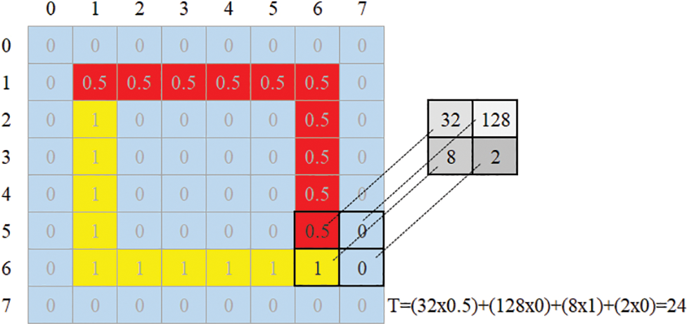
Figure 4: Filter weights and their corresponding image pixels

Contour tracing is basically a morphological image processing concept and deals with tracing the boundaries generally in binary images. In such tracing algorithms, defining start-stop criteria, labeling boundary points, and determining the next moving directions are the main issues to be considered. Problems with identifying neighboring pixels, unnecessary and repetitive movement, and detecting stop criteria are the main challenges in these algorithms. In this study, the binary image to be processed has intensity values of 0 and 1 for the background and object pixels, respectively. While processing the image, an intensity value of 0.5 was assigned to the detected contour points. In a particular filter position, each point at the 2 × 2 region may have one of the three density values as 0, 1, or 0.5. Therefore, 34 = 81 different neighborhood cases occur, some of which are shown in Fig. 5. In the figure, black, white, and labeled pixels are shown in blue, yellow, and red colors for clarity, respectively. When the filter overlaps any neighborhood cases in Fig. 5, the T values obtained by multiplying the corresponding values of the 2 × 2 region and the filter coefficients are also given next to the cases.

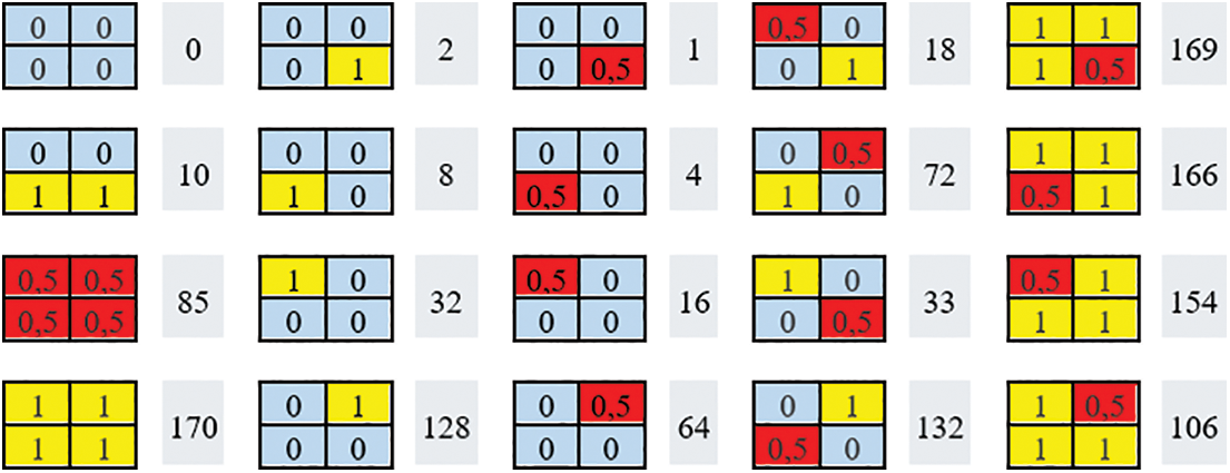
Figure 5: Samples for some neighborhood cases and calculated corresponding T values

3.2 Tracing Direction and Pixel Labeling

There are two terms related to tracing action: tracing direction and tracing movement. Tracing direction refers to the main path of tracing, such as clockwise (CW) and counterclockwise (CCW). Tracing movement, on the other hand, determines the next pixel to be traced in the right, down, left, or up direction while at a certain position in the image. Determining the next movement and the pixel to be labeled depends on the tracing direction. CW and CCW are the two tracing directions. Most neighborhood cases at filter locations were not encountered during contour tracing. Therefore, possible encountered 2 × 2 image pixel values for four tracing movements (right, down, left, and up) and stopping cases in CW and CCW tracing are given in Fig. 6. Our tracing algorithm follows the steps below.

1.    Decide on the tracing direction (CW or CCW).

2.    Search the starting point of the object boundary from the outside of the object in a circular manner with certain angle intervals and position the filter according to the detected starting point as described in Sections 3.3 and 3.4.

3.    Calculate the T value for the filter position determined in step 1.

4.    Determine the pixel to be labeled and the tracing movement of the filter using the calculated T value according to the decided tracing direction (CW or CCW).

5.    Repeat steps 3 and 4 until reaching the starting point or no pixel left to be labeled. If the starting point is reached (closed-loop condition), stop the tracing. If the no-pixel-to-be-labeled condition occurs, go to the starting point, change the tracing direction decided in step 1 and repeat steps 3 and 4 until no pixel is left.

6.    Continue searching for the next starting point in a circular manner by increasing the angle. If all the pixels are already labeled as object points, stop the overall tracing. Otherwise, go to step 3.

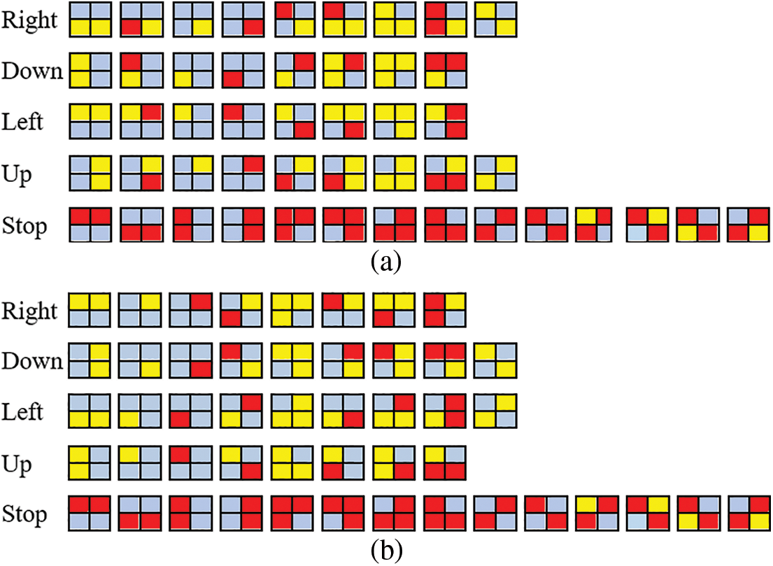
Figure 6: Next tracing movements and corresponding neighborhood cases represented with 2 × 2 image pixel values for (a) CW and (b) CCW tracing

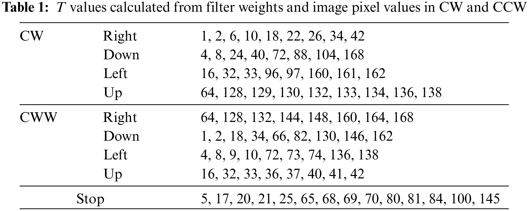
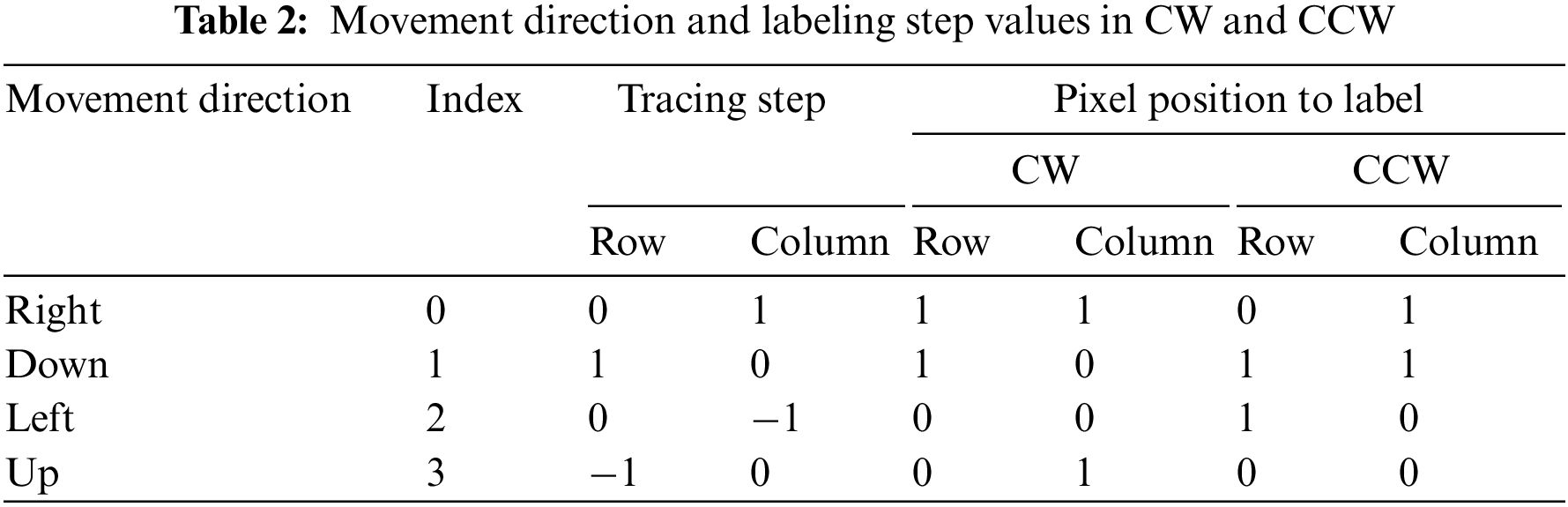
Two arrays, named SCOREandINDEX and DRCandLBL, were used to maximize the computational speed of simultaneous tracing and labeling. The structures of the arrays used in the tracing algorithm are shown in Figs. 7 and 8 SCOREandINDEX has two main sub-arrays, one holding the CW and the other CWW score values. Each main sub-array also consists of 5 separate sub-arrays containing T values, which indicate the right (R), down (D), left (L), and up (U) movement directions and stopping criteria (S). The calculated T values of the movement directions according to Fig. 6 are given in Table 1. The T values of stopping are common for both CW and CWW tracing. The T value produced by the filter at a certain image position is searched in either the first or the second main sub-array in the SCOREandINDEX array, depending on the tracing direction (CW or CWW). Depending on whether the tracing direction is CW or CWW, all possible movement direction and labeling step values are given in Table 2. For example, if the tracing direction is CW and the T value produced by the filter is 97, the first main sub-array (since it is CW tracing) in the SCOREandINDEX array is searched, and this T value is found in the L (left) sub-array. Since the order index for L in the first main sub-array is 2 (order indices are 0, 1, 2, 3, and 4 for R, D, L, U, and S, respectively), the direction of movement and the position of the pixel to be labeled are obtained in the index 2 in the DRCandLBL array including movement direction and labeling row and column step values.

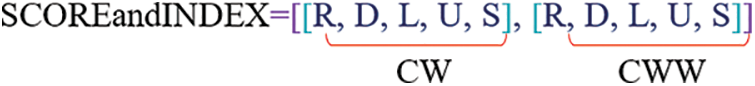
Figure 7: Structure of the SCOREandINDEX array

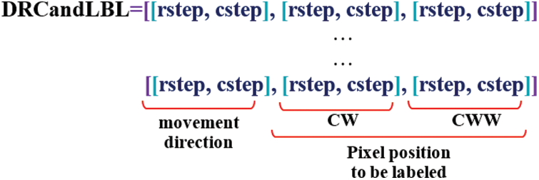
Figure 8: Structure of the direction and labeling array

3.3 Tracing Closed-Loop and Open-Loop Paths

In the closed-loop path case, the tracing is executed CW or CCW along the outer boundary and ends when the starting point is reached. In the open-loop path case, tracing is mostly performed in two steps, as the starting point may not be the first point of the boundary. Therefore, tracing is done for the first part of the path until the stopping criterion is met, and then the remaining part is followed in the reverse direction from the starting point. Thus, in any open-loop case, the boundary points can be obtained sequentially, no matter which point is chosen as the starting point. In Fig. 9, the tracing steps for both closed-loop and open-loop cases are given. Sample tracing results are given in Figs. 10 and 11 [25] for open-loop and closed-loop paths, respectively.

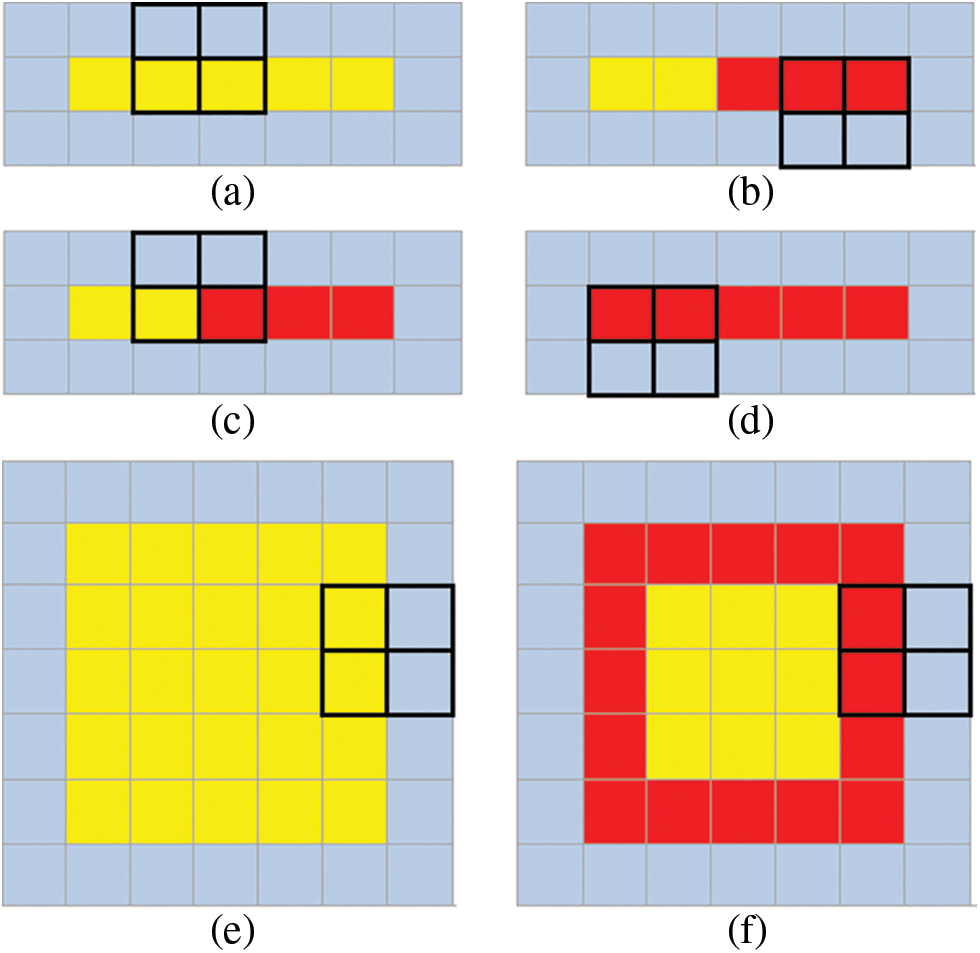
Figure 9: Sample tracing steps for open-loop path (a)–(d) and closed-loop path (e)–(f). In the open-loop case, first, if CW is preferred and then CCW tracing is performed, while in the closed-loop case, only CW or CCW tracing is performed

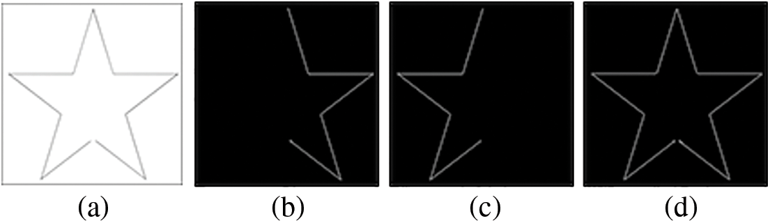
Figure 10: (a) Open-loop sample to be traced, the results of (b) CW tracing for the first part of the boundary, (c) CCW tracing for the remaining part, and (d) overall boundary

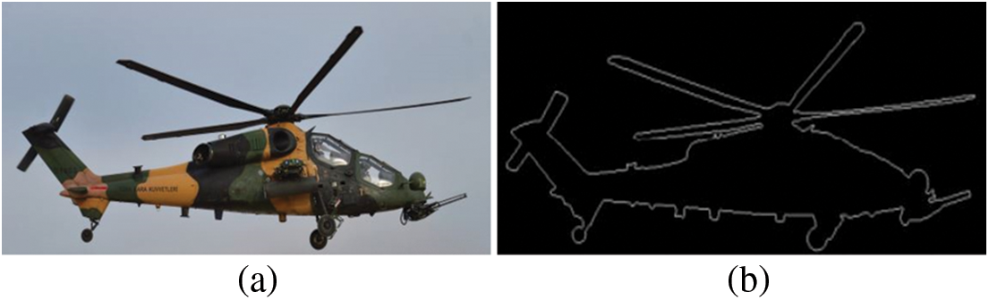
Figure 11: (a) Closed-loop sample to be traced, (b) the results of tracing

3.4 Limitations of the Algorithm and Solution

The scoring algorithm fails in case of more than one discontinuity caused by deformation at the outer boundaries of objects due to reflection or different shooting angles. As seen in the result in Fig. 12b, it cannot follow the entire path in the case with more than one discontinuity (Fig. 12a). As a solution to this deficiency occurs with discontinuity, it is necessary to find the starting point for each split border segment.

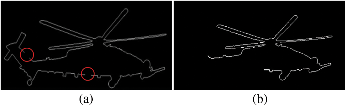
Figure 12: (a) Manually applied deformation (b) tracing result with the scoring method

We suggested that possible starting points of object boundary segments could be reached from the outside of the object in a circular manner with certain angle intervals. The circle surrounding the object and the search directions to find the first edge points are shown in Fig. 13a as a representative drawing. Once the starting point of a segment is determined with the angular approach, the border tracing process starts with the scoring method. Therefore, the number of starting points to be determined using angular search is equal to the number of border segments. For example, if there is no border discontinuity, then using the first starting point will suffice to trace all the paths.

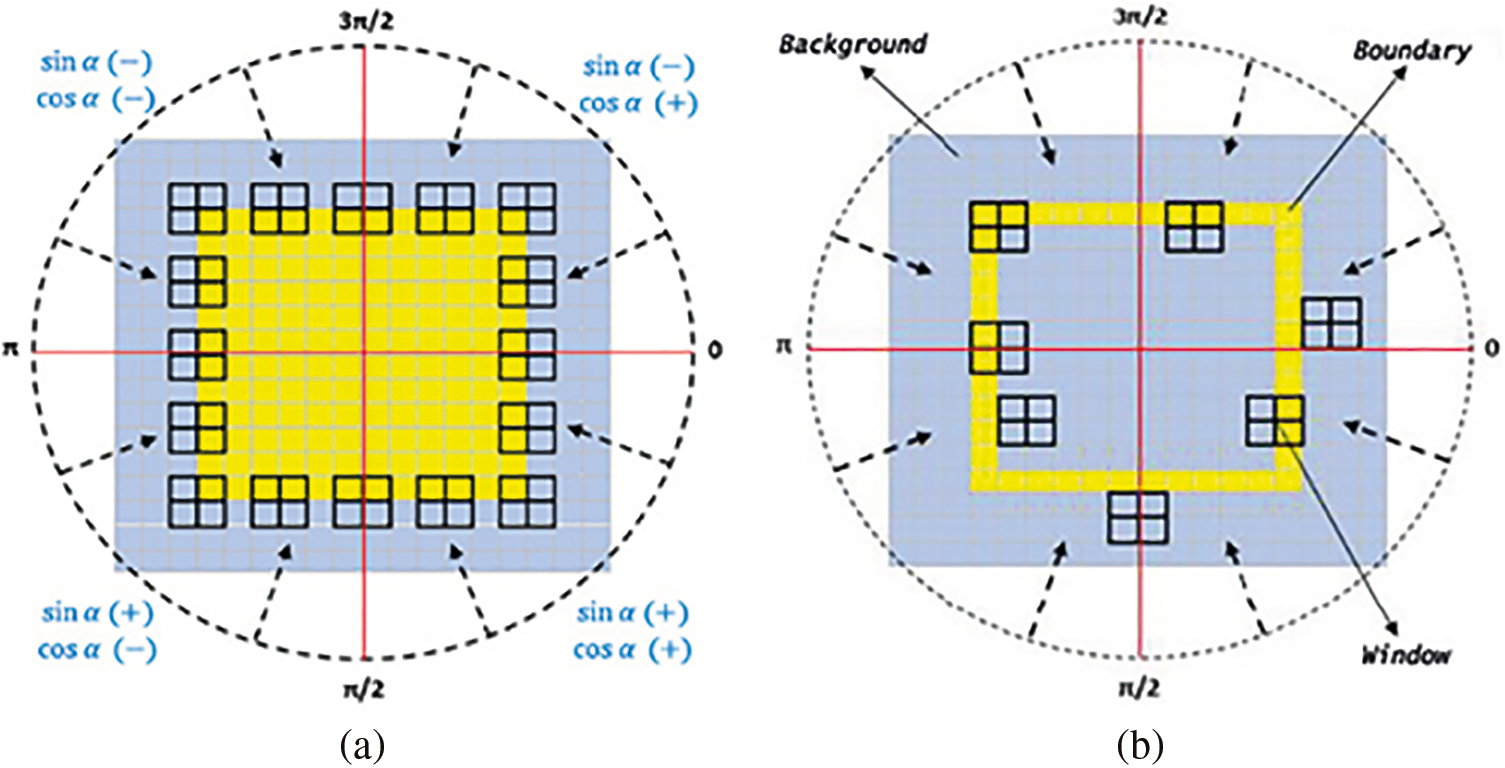
Figure 13: Samples for (a) correct and (b) wrong positioning of the filter window according to the detected tracing starting points

The radius (r) of the circle is calculated according to Eq. (7) where (Ox, Oy) and (Px, Py) are the center of the object and the extreme point position relative to the object center, respectively. c is a margin with at least one-pixel length needed for the border point search algorithm.

rx=Px−Ox,ry=Py−Oy,r=rx2+ry2+c(7)

Correct positioning of the filter window for the starting point is crucial for proper tracing. The leftmost point of the filter window should be located at (x, y), which is calculated as follow:

x=x0+floor(sinα),y=y0+floor(cosα)(8)

where (x0, y0) is the detected starting point, x and y are the vertical (row axis) and horizontal (column axis), and α is the angle that the line joining a point on the circle and the object center makes with the horizontal (y) axis. In Fig. 13a, the signs of the values produced by the sine and cosine functions according to the regions and samples for correct window positioning are given. In Eq. (8), the floor function produces 0 and −1 for values in the range [0, 1) and [−1, 0), respectively. Thus, the window is positioned correctly according to the detected starting point. Samples for the wrong positioning of the window are given in Fig. 13b.

Although the angular search method can be used for tracing purposes as well as starting point detection, it produces incomplete results for hard samples, similar to the scoring method. Therefore, we used the angular approach only for detecting the starting points of segments. It is seen in Fig. 14b that the tracing is completed as a result of using the two methods together.

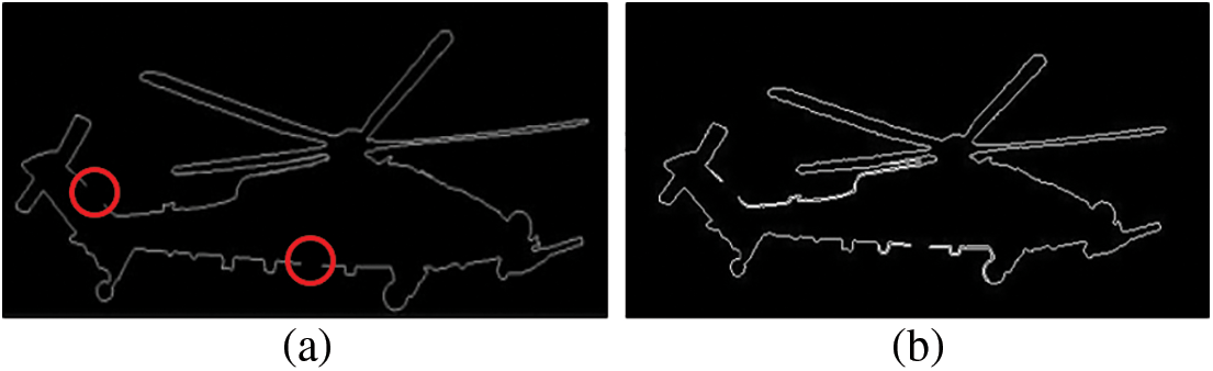
Figure 14: (a) Manually deformation (b) tracing result of both Scoring and Angular methods together

4  Experiments for Shape Reconstruction

In this section, experiments for reconstructing the object shape with Bézier and B-spline curves using the object boundary points obtained sequentially by our contour tracing algorithm are explained. If the original image containing the object to be traced is a color image, then the image is first converted to gray, and then a Gaussian filter is used to smooth out sharp transitions and remove noise. In addition, the image is converted to binary format using a threshold. Since the proposed contour tracing algorithm is developed by assuming that the object has white pixels, the negative of the image with white background and black object color are taken. After the pre-processing operations, the outer boundary points of the object were obtained sequentially with their positions by following the border points of the object with the proposed algorithm. Then diluting the sequential points, the object’s shape was reconstructed using Bézier and B-spline curves with these positions. These curves were compared in terms of their ability to represent the object’s shape. The flowchart of the preprocessing and reconstruction steps is given in Fig. 15.

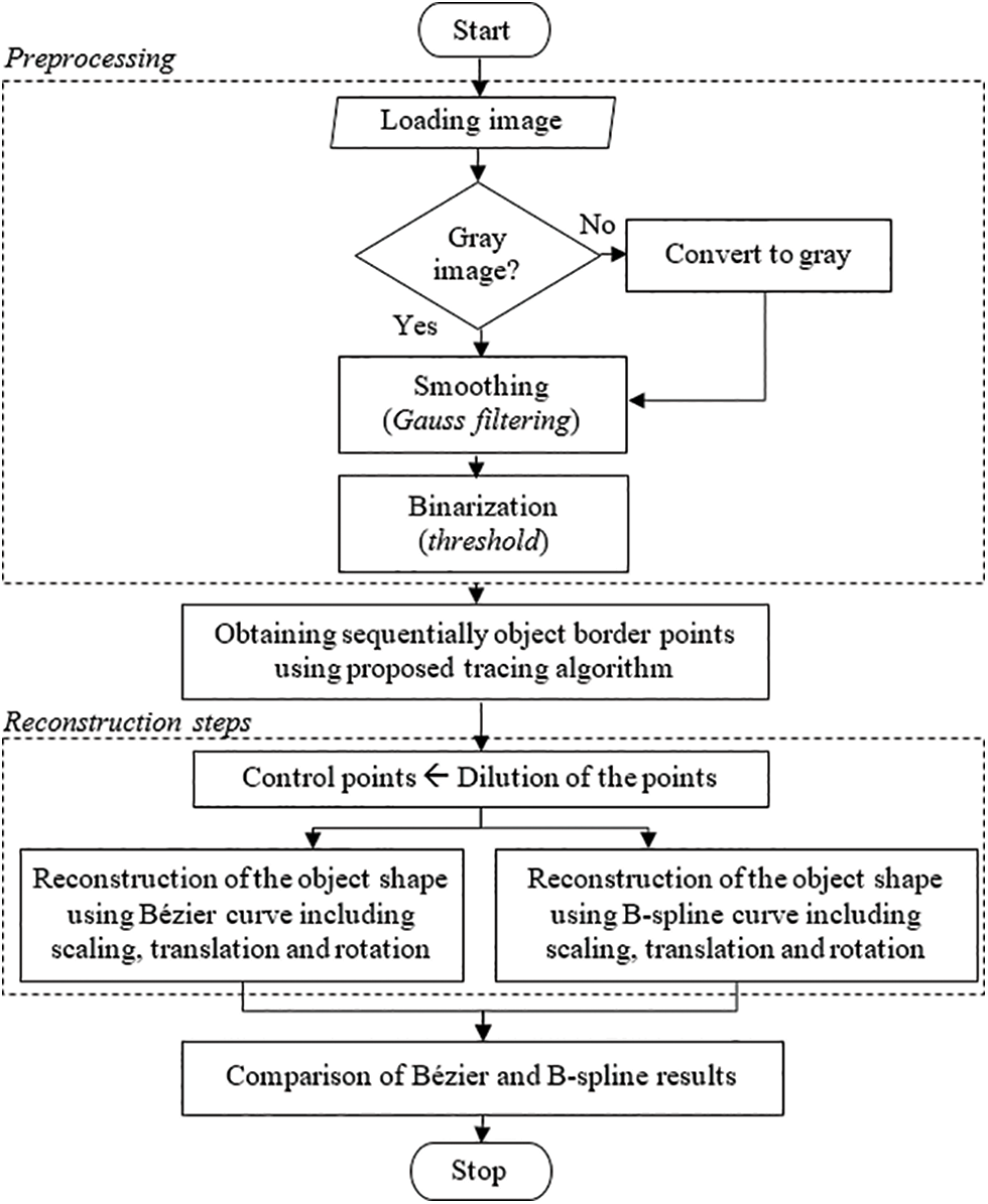
Figure 15: Flowchart of the experimental studies

In this study, the object shape is reconstructed using the border points obtained by the proposed boundary tracing method as control points in parametric curves. The reconstructed and original objects were compared with the area similarity ratio (AS%). The area similarity percentage is calculated by Eq. (9).

AS%=Area within Reconstructed ShapeOriginal Object Area×100(9)

where the area is the number of pixels inside the closed curve.

The contour tracing algorithm we developed has been compared with other commercially used algorithms. For this, the ratio of boundary points detected by the tracing algorithm to the points of the original object boundary is used. The intersection ratio (IP%) is calculated by Eq. (10).

IP%=number of border points in the algorithm outputnumber of original border points×100(10)

4.1 Contour Tracing and Reconstruction Experiments

For the first reconstruction experiment, we used a 2D binary image [26] of four chess pieces. Binary images were processed with the developed tracing algorithm, and the outputs are given in Fig. 16. The results show that the edge points detected by the tracing algorithm highly represent the outer boundaries of the objects.

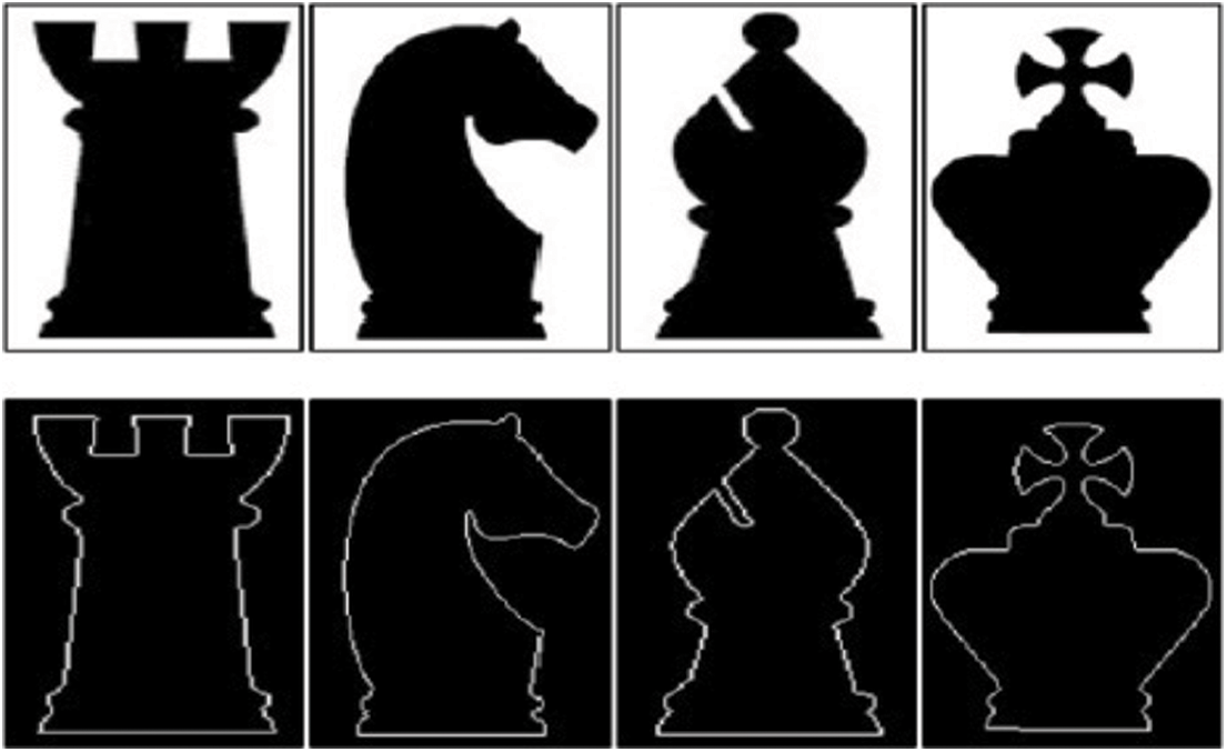
Figure 16: First row: Binary images, second row: Boundaries detected by contour tracing algorithm

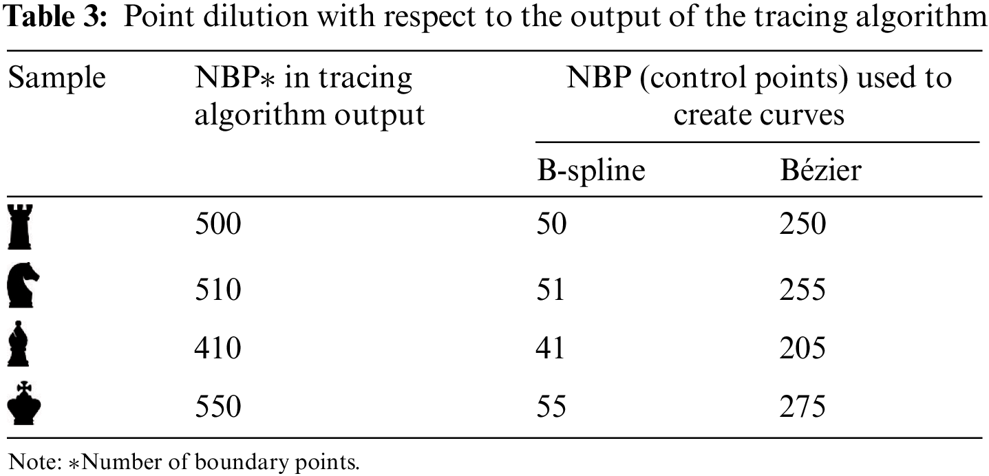
By the proposed contour tracing algorithm, the border points of the objects in the image were obtained sequentially. These obtained points were diluted by 90% and 50% and determined as control points for B-spline and Bézier curves, respectively. Using these control points, the shapes of the objects were reconstructed with the parametric curves. The reconstructed object shapes of B-spline and Bézier are given in Fig. 17. In Table 3, in the second column of the table, the number of points detected by the tracing algorithm is given. In the third and fourth columns, the numbers of control points obtained by dilution can be seen for B-spline and Bézier, respectively. The reconstructed results show that B-spline curves better represent the input image than Bézier curves due to their local segment control ability.

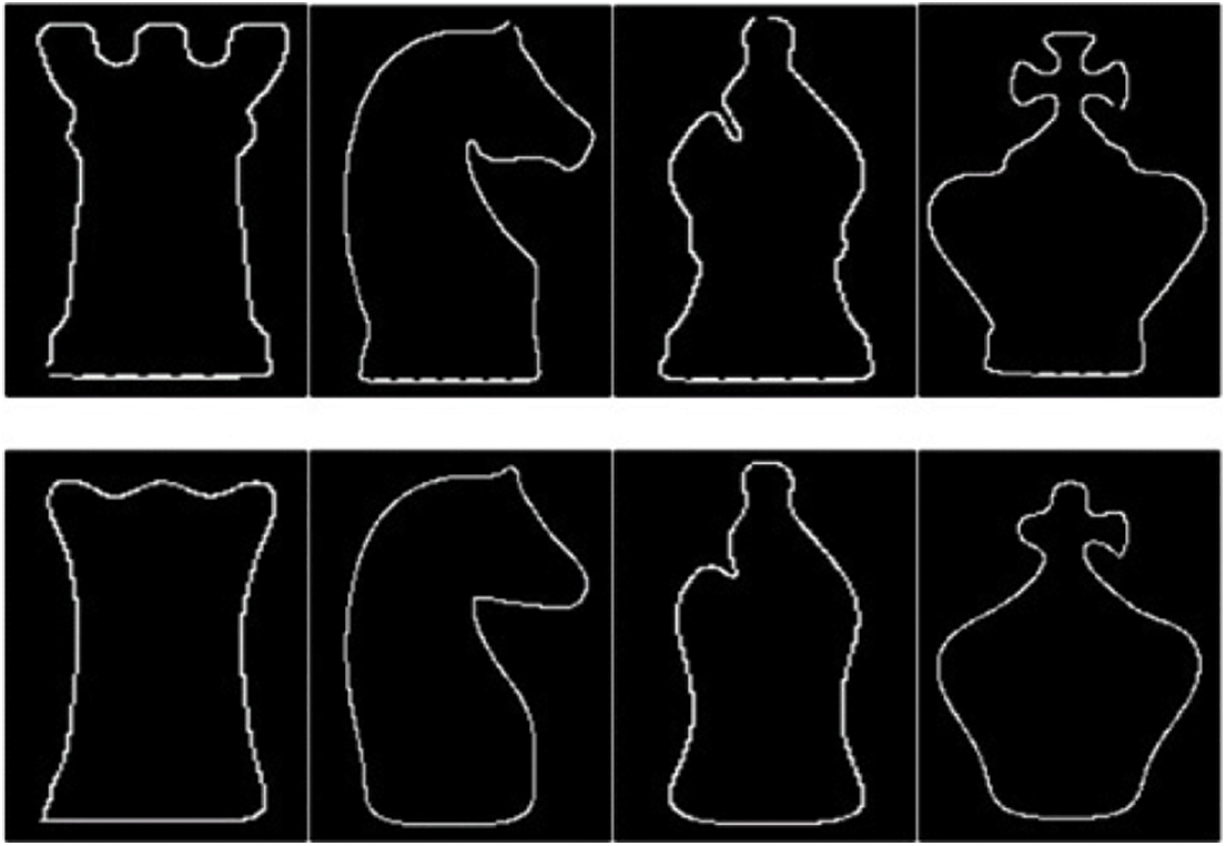
Figure 17: Reconstruction using B-spline curves (first row) and Bézier curves

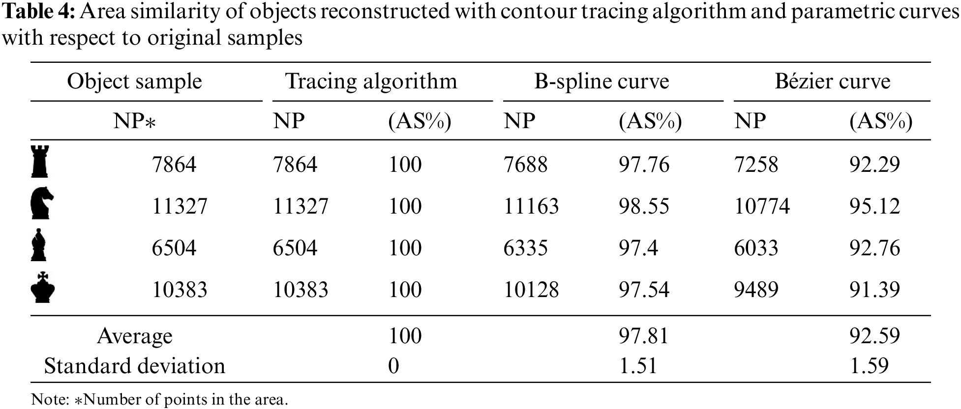
One of the methods used to measure the similarity between two closed curves is area similarity. In this study, in order to compare the area similarity, first, the object boundary points were obtained from the original object images (Fig. 18a) with the contour tracing algorithm. The algorithm’s output is given in Fig. 18b. Then, the object shapes were reconstructed with B-spline and Bézier curves using the control points selected from the tracing algorithm output points. The results of B-spline and Bézier are given in Figs. 18c and 18d, respectively. The inner pixels of the reconstructed object shape were assigned white (1), and the background pixels black (0). Then, the area of each of the original objects was compared with the areas of the reconstructed objects with the contour tracing algorithm and parametric curves. The similarity values can be seen in Table 4. While the contour tracing algorithm we developed in area similarity showed full similarity to the original image, the least similarity occurred in the Bézier curve, as expected due to the lack of local control capability.

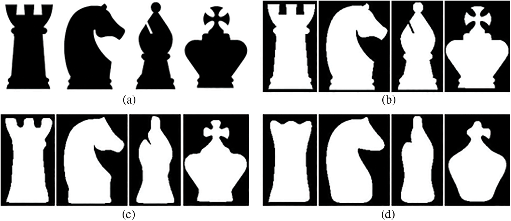
Figure 18: (a) Input images, (b) Object images obtained by proposed contour tracing algorithm, areas bounded by the object shapes reconstructed using (c) B-spline curve, and (d) Bézier curve

In computer vision, it may be necessary to segment objects and reconstruct them in different scales and orientations. Using parametric curves, reconstruction operations, including a different translation, scaling, and rotation can be easily performed with less memory requirement. Translation, scaling, and rotation operations are performed by changing the locations of the control points selected from the boundary points. Scaling is a linear transformation that enlarges or reduces images by a scale factor that is the same in all directions. In this context, it is realized by moving the control points away from or closer to the object center. In the process of rotation, as in the scaling process, all control points are rotated with a certain angle relative to the object center. In the translation process, control points are simply shifted to a certain pixel distance. In this study, the reconstruction results obtained by applying scaling and rotation together of an object [27] are shown in Fig. 19. The translation results also are given in Fig. 20. As expected, the reconstruction output obtained with the Bézier curve as a result of scaling and rotating the object showed more deformation at the boundaries.

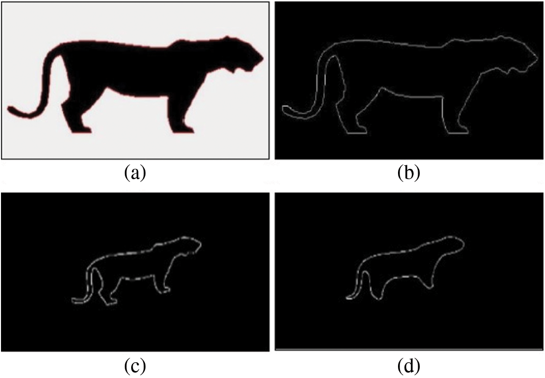
Figure 19: (a) Input image, (b) contour tracing algorithm result, results of (c) B-spline, and (d) Bézier

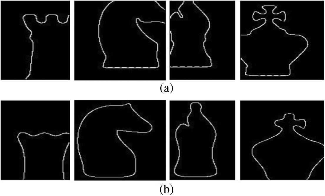
Figure 20: Reconstruction of outer boundaries of objects with (a) B-spline and (b) Bézier after translating the control points

Deformations may occur at the borders of the objects in the image due to different reasons, such as reflection or shooting angles. In this study, firstly, B-spline and Bézier curves were created by using the control points selected as linearly distributed from the object boundary obtained by the algorithm we proposed. Then, manually created boundary deformation was eliminated by using these curves. Fig. 21a was obtained by manually deleting some points on the object’s border [28]. As seen in Figs. 21b and 21c, the missing part of the object was completed by using B-spline and Bézier curves.

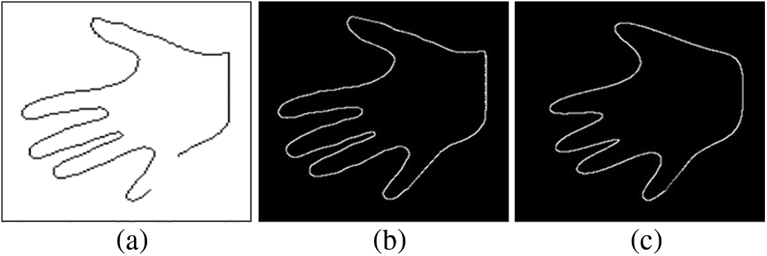
Figure 21: (a) Image obtained by manually deleting some points, (b) B-spline, and (c) Bézier reconstruction results

4.2 Challenges in Reconstruction Process

The shape reconstruction process has some challenging issues. The main challenges are:

•   To reconstruct the shape with parametric curves such as B-spline and Bézier, the object boundary points must be sequential. The outputs of the existing commercial contour tracing functions are not sequential. Therefore, in this study, an algorithm that obtains the boundary points sequentially has been developed.

•   The resulting points should belong to the outer boundaries that determine the object’s shape. Since most of the existing functions also find points belonging to the internal texture of the object, the points obtained by these functions cannot be used as control points for parametric curves.

•   Compared to the original, it requires a certain number of points to reconstruct the shape with satisfactory quality. The fewer control points used, the less representativeness of the reconstructed shape. On the other hand, using more points will increase the computational and memory cost.

4.3 Comparison with Existing Algorithms

In order to determine the processing time performance of the algorithm we developed, it was compared with findContours [29] and Moore’s boundary tracing algorithm [30] in OpenCV, which are widely used in computer vision applications. For this, 100 images obtained from the brain image dataset [31] were used. These images were converted to binary format. This dataset is preferred because boundary tracing algorithms are generally used for images containing a single object. Some sample images used for the test are shown in Fig. 22a. All images in the dataset are time tested with two algorithms of OpenCV and the algorithm we proposed. The 5-fold test process was carried out on images. For 100 images, the processing average and standard deviation values of findContours, Moore, and proposed algorithms are 0.37 ± 0.02, 3.82 ± 0.41, and 10.36 ± 0.15, respectively. Although the proposed algorithm seems to run slower than other algorithms, its processing time performance is satisfactory, given that the OpenCV functions run in an environment optimized for data structure and memory management [32]. In addition, our algorithm is better than other algorithms in terms of outer boundary tracing. findContours also detected some interior points in the object area, as shown in Fig. 22b. In Moore’s boundary tracing algorithm, as seen in Fig. 22c, the whole borders of some images could not be obtained. On the other hand, our algorithm completely found the outer boundaries of objects in all images (Fig. 22d). In order to reconstruct an object shape using parametric curves such as Bézier and B-splines at different scales and orientations, the boundary points of the object must be obtained sequentially. Therefore, the points determined by findContours and Moore’s algorithms do not produce output in a format suitable for use as control points in parametric curves.

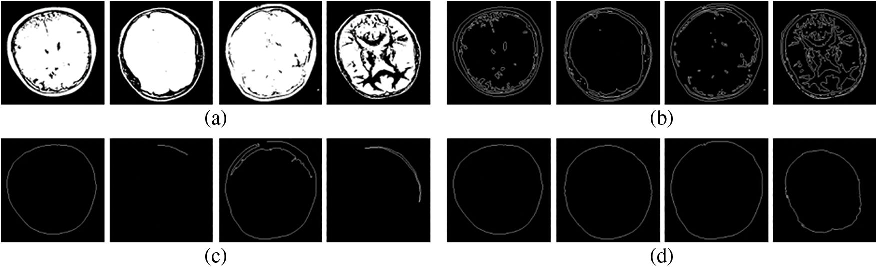
Figure 22: (a) Binary input images, results of (b) findContours (c) Moore (d) Proposed algorithm

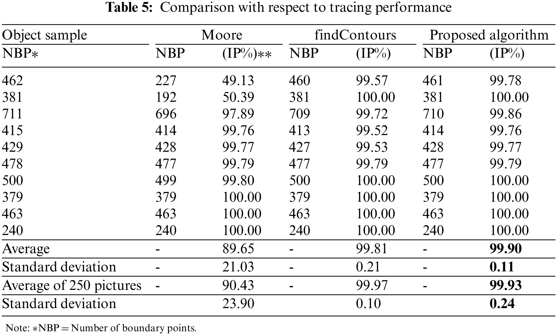
To measure the boundary tracing performance of the proposed algorithm, 250 cancer cell images [33] were used. After the borders of the objects in the images were obtained using the Canny edge detection algorithm, these borders were reduced to a single pixel width. Results obtained with findContours (Fig. 23b), Moore (Fig. 23c), and proposed (Fig. 23d) algorithms are shown in Table 5. It can be seen that the sequential boundary points obtained with our algorithm overlap with the boundary points of the object. The results of 10 selected samples are given in Table 5. The last row shows the mean and standard deviation results for 250 images. Accordingly, our proposed algorithm obtained better results than Moore’s while close to findContours.

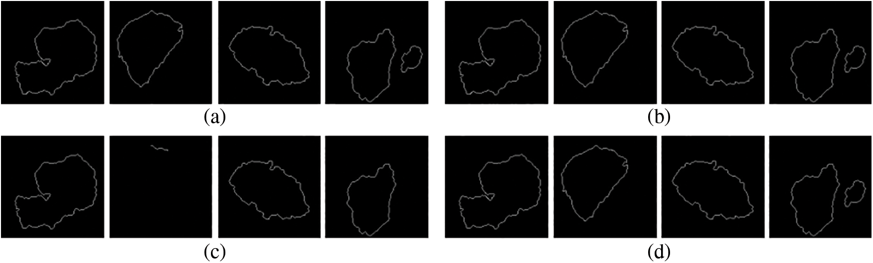
Figure 23: (a) Binary input images, results of (b) findContours (c) Moore (d) Proposed algorithm

5  Conclusion

Parametric curves are frequently preferred in many fields, such as image processing, CAD, and CAM, especially computer graphics. Parametric curves such as Bézier and B-spline are defined by a series of points called control points. The sequence of these control points also determines the shape of the curve. Therefore, a new contour tracing algorithm is proposed to sequentially obtain the points of the outer boundary of the object. The proposed algorithm, unlike the methods in the literature, is implemented by using a filter containing weights and a circle surrounding the object in the image. The algorithm consists of three main parts: detecting the starting points of tracing, following the boundary, and stopping the tracing. The starting point for tracing is determined by scanning along a line in the direction of the center from the circle surrounding the object, and then contour tracing is performed with the scoring method. The computational time of the contour tracing algorithm was dramatically reduced as all possible values generated by filtering and the corresponding moving direction and labeling information are pre-recorded in an array. With the proposed algorithm, the boundary points of the objects were obtained sequentially, and these points were diluted to form control points for Bézier and B-spline. Finally, the object shapes were reconstructed using B-spline and Bézier, including a different translation, scaling, and orientation.

According to the developed tracing algorithm results, the tracing algorithm can successfully follow the entire boundary of the object even in the presence of more than one discontinuity. The areas formed by the curves obtained using B-spline and Bézier were compared with the original object area. B-spline results were found to represent the object better than Bézier. It has also been demonstrated that B-spline requires much fewer control points for reconstruction compared to Bézier. In addition, the reconstruction outputs obtained with the Bézier showed more deformation at the boundaries compared to the B-spline. While B-spline can provide local change, Bézier allows only global control. Operations such as adding, deleting, or relocating a control point to the curve affect the entire curve in Bézier but only a small part of the curve in B-spline. Therefore, Bézier curves cause much loss in the boundary details of the object, while B-spline curves better represent the object boundary. On the other hand, it has been shown that the deformations caused by different reasons on the border of the object can be eliminated by using Bézier and B-splines, which are created using the control points obtained with the boundary tracing algorithm. According to the comparison results made with findContours and Moore algorithms in the OpenCV library, which are widely used in computer vision applications, our algorithm performs better than the Moore method and is close to the findContours algorithm in terms of border tracing.

Funding Statement: The authors received no specific funding for this study.

Conflicts of Interest: The authors declare that they have no conflicts of interest to report regarding the present study.

References

1. S. Cuomo, A. Galletti, G. Giunta and L. Marcellino, “Reconstruction of implicit curves and surfaces via RBF interpolation,” Applied Numerical Mathematics, vol. 116, pp. 157–171, 2017. [Google Scholar]
2. G. Farin, Curves and Surfaces for CAGD: A Practical Guide, Amsterdam, The Netherlands: Elsevier B.V., 2002. [Online]. Available: https://www.sciencedirect.com/book/9781558607378/curves-and-surfaces-for-cagd#book-description. [Google Scholar]
3. A. Lastra, “Architectural form-finding through parametric geometry,” Nexus Network Journal, vol. 24, pp. 271–277, 2022. [Google Scholar]
4. M. Dixit and S. Silakari, “Utility of parametric curves in image processing applications,” International Journal of Signal Processing, Image Processing and Pattern Recognition, vol. 8, no. 7, pp. 317–326, 2015. [Google Scholar]
5. O. R. Vincent and O. Folorunso, “A descriptive algorithm for sobel image edge detection,” in Proc. of Informing Science & IT Education Conf. (InSITE), California, USA, pp. 97–107, 2009. [Google Scholar]
6. M. Mittal, A. Verma, I. Kaur, B. Kaur, M. Sharma et al., “An efficient edge detection approach to provide better edge connectivity for image analysis,” IEEE Access, vol. 7, pp. 33240–33255, 2019. [Google Scholar]
7. Y. Liu, Z. Xie and H. Liu, “An adaptive and robust edge detection method based on edge proportion statistics,” IEEE Transactions on Image Processing, vol. 29, pp. 5206–5215, 2020. [Google Scholar]
8. L. Sun and T. Huang, “A new boundary tracing algorithm of the contour of objects in the binary image,” Computer Modellıng & New Technologıes, vol. 17, no. 5A, pp. 63–67, 2013. [Google Scholar]
9. W. Zhong, X. Luo, F. Ding and Y. Cai, “A real-time interpolator for parametric curves,” International Journal of Machine Tools and Manufacture, vol. 125, pp. 133–145, 2018. [Google Scholar]
10. V. Hassani and S. V. Lande, “Path planning for marine vehicles using Bézier curves,” International Federation of Automatic Control (IFAC)-PapersOnLine, vol. 51, no. 29, pp. 305–310, 2018. [Google Scholar]
11. F. Díaz Moreno, “Hand drawing in the definition of the first digital curves,” Nexus Network Journal, vol. 22, no. 3, pp. 755–775, 2020. [Google Scholar]
12. O. Stelia, L. Potapenko and I. Sirenko, “Computer realizations of the cubic parametric spline curve of Bezier type,” International Journal of Computing, vol. 18, no. 4, pp. 422–430, 2019. [Google Scholar]
13. A. Chakwizira, A. Ahlgren, L. Knutsson and R. Wirestam, “Non-parametric deconvolution using Bézier curves for quantification of cerebral perfusion in dynamic susceptibility contrast MRI,” Magnetic Resonance Materials in Physics, Biology and Medicine, vol. 35, pp. 1–14, 2022. [Google Scholar]
14. O. Coskun and H. S. Turkmen, “Multi-objective optimization of variable stiffness laminated plates modeled using bézier curves,” Composite Structures, vol. 279, pp. 114814, 2022. [Google Scholar]
15. W. Neubauer and J. Linhart, “Approximating and distinguishing ostracoda by the use of B-splines,” Berichte des Institutes für Erdwissenschaften Karl-Franzens-Universität Graz, vol. 13, pp. 21–42, 2008. [Google Scholar]
16. M. Z. Hussain, S. Abbas and M. Irshad, “Quadratic trigonometric B-spline for image interpolation using GA,” PloS One, vol. 12, no. 6, pp. e0179721, 2017. [Google Scholar]
17. D. Auger, Q. Wang, J. Trevelyan, S. Huang and W. Zhao, “Investigating the quality inspection process of offshore wind turbine blades using B-spline surfaces,” Measurement, vol. 115, pp. 162–172, 2018. [Google Scholar]
18. C. Balta, S. Öztürk, M. Kuncanand and I. Kandilli, “Dynamic centripetal parameterization method for B-spline curve interpolation,” IEEE Access, vol. 8, pp. 589–598, 2019. [Google Scholar]
19. M. Ameer, M. Abbas, T. Abdeljawad and T. Nazir, “A novel generalization of Bézier-like curves and surfaces with shape parameters,” Mathematics, vol. 10, no. 3, pp. 376, 2022. [Google Scholar]
20. M. Abbas, A. A. Majid and J. M. Ali, “Monotonicity-preserving C2 rational cubic spline for monotone data,” Applied Mathematics and Computation, vol. 219, no. 6, pp. 2885–2895, 2012. [Google Scholar]
21. S. Öztürk, C. Balta and M. Kuncan, “Comparison of parameterization methods used for B-spline curve interpolation,” European Journal of Technique (EJT), vol. 7, no. 1, pp. 21–32, 2017. [Google Scholar]
22. C. G. Lim, “A universal parametrization in B-spline curve and surface interpolation,” Computer Aided Geometric Design, vol. 16, no. 5, pp. 407–422, 1999. [Google Scholar]
23. C. De Boor, “On calculating with B-splines,” Journal of Aproximate Theory, vol. 6, pp. 50–62, 1972. [Google Scholar]
24. A. Kaehler and G. Bradski, “Filters and convolution,” in Learning OpenCV 3: Computer vision in C++ with the OpenCV library, 1st ed., Sebastopol, CA, USA: O’Reilly Media, Inc., pp. 249–349, 2016. [Google Scholar]
25. I. Demir, “Transformation of the Turkish Defense Industry,” Insight Turkey, vol. 22, no. 3, pp. 17–40, 2020. [Google Scholar]
26. Y. Batko and V. Dyminsky, “Fast contour tracing algorithm based on a backward contour tracing method,” in Int. Conf. “Advanced Computer Information Technologies”, Ceske Budejovice, Czechia, vol. 2300, pp. 219–222, 2018. [Google Scholar]
27. J. Rao, J. Lin, S. Xu and S. Lin, “A new intelligent contour tracking algorithm in binary image,” in 2012 Fourth Int. Conf. on Digital Home, Guangzhou, China, IEEE, pp. 18–22, 2012. [Google Scholar]
28. N. L. Narappanawar, B. M. Rao, T. Srikanth and M. A. Joshi, “Vector algebra based tracıng of external and internal boundary of an object in bınary images,” Journal of Advances in Engineering Science, vol. 3, pp. 57–70, 2010. [Google Scholar]
29. V. M. Garcia-Molla, P. Alonso-Jordá and R. García-Laguía, “Parallel border tracking in binary images using GPUs,” The Journal of Supercomputing, vol. 78, pp. 9817–9839, 2022. [Google Scholar]
30. S. Biswas and R. Hazra, “Robust edge detection based on modified Moore-neighbor,” Optik, vol. 168, pp. 931–943, 2018. [Google Scholar]
31. D. Padalia, K. Vora and T. Mind, Denoising Brain Tumor, California, USA: Kaggle Inc., 2022. [Online]. Available: https://www.kaggle.com/datasets/dishantpadalia/denoising-brain-tumor. [Google Scholar]
32. “OpenCV (Open source computer vision library) introduction,” 2022. [Online]. Available: https://docs.opencv.org/4.x/d1/dfb/intro.html. [Google Scholar]
33. H. Y. Chai, L. K. Wee and E. Supriyanto, “Edge detection in ultrasound images using speckle reducing anisotropic diffusion in canny edge detector framewor,” in Proc. of the 15th WSEAS Int. Conf. on Systems, Corfu Island, Greece, pp. 226–231, 2011. [Google Scholar]
Cite This Article
Copyright © 2023 The Author(s). Published by Tech Science Press.
This work is licensed under a Creative Commons Attribution 4.0 International License , which permits unrestricted use, distribution, and reproduction in any medium, provided the original work is properly cited.
Downloads
Citation Tools