Dynamic Behavior-Based Churn Forecasts in the Insurance Sector

1  Introduction

Client churn refers to the fall of customers in Customer Relationship Management (CRM). It is the occurrence of a customer discontinuing the avail of a product or service provided by the organization. Customer churn is named customer attrition. it is among the most critical issues that reduce a company’s profit. Business intelligence procedures for locating customers who want to change from one company to another company can be described as customer churn. In contrast, the retention rate assesses the retained clients [1].

1.1 Preliminary Understanding

Churn forecasting models will aid in the development of customer intervention strategies by identifying churners earlier. This is essentially a classification problem. Each customer must be classified as a potential churner or a non-churner [2].

1.2 Motivation

Controlling customer churn is one of the primary growth pillars of the financial service sector. Due to tough competition in the market, there is lots of choice from a number of service providers. The customers have the freedom to switch over to competitors due to many or even one bad experience. There is a lot of research work and modeling techniques performed to pursue features affecting customer churn, but in most cases, there is a less technical and specific enough approach to resolve the problem.

1.3 Why is Attrition so Critical?

When customers are migrating, companies face not only the loss of revenue from those customers but also the high cost of acquiring new customers. No regardless of how excellent a firm’s product or service and it must keep track of its customer churn rate. Customers are the core of the business, so businesses must understand churn if they want to develop and adapt to meet the requirements of their buyers [3].

In the insurance industry, a customer is described as a churner when he stops doing income-generating actions for 30 days just after policy coverage expires. These days are referred to as the inactivity period. To develop a model to forecast churning, the customer's behavior during the time period preceding the idleness period, known as the observation period, is examined. In some words, some characteristics that could encompass the consumer during the monitoring time are transferred into a binary categorization method to be competent with the labels (churn, non-churn) . This model's outcome can formally have illustrated as follows: ChurnScore (X, d) = p (class = Churner | X [d–30, d-1]).

Here d is the present day and X is a multivariate time series data representing the client’s daily behavior during the period of observation. Furthermore, this method will recognize them as unsafe customers with a more churn score (>=0.9), indicating that no retention initiative should target them in Fig. 1. In constructing a model that finds potential churners, this research explores different automatic methods for extracting significant attributes from X [d30; d-1] [4].

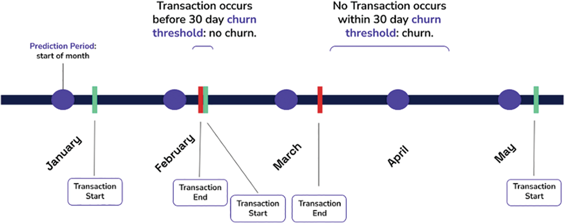
Figure 1: 30 days’ time line window for daily churn prediction model

When this period of inactivity or behavioral change exceeds a certain threshold, the customer is considered a churned customer. The timeframe is the period that is specified as the threshold of the lack of activity date during such a process.

1.4 Main Contributions

1) Addressing the problem of daily forecasting based on dynamic customer behavior on a daily basis.

2) Six approaches to daily churn prediction via customer feature selection-based strategy and deep learning approaches.

3) Proposed CELM outperforms all other methods in terms of performance accuracy. The Customized word is instigating in the existing ELMs to initiate the Customized extreme learning machine to reduce structural risk (CELM).

4) Relate the effectiveness of these methods to prior monthly forecasts based on a big dataset obtained from the Health insurance dataset in Kaggle’s catalog, which demonstrated that our model outperformed previous representations in terms of forecasting churners earlier and further accurately.

This paper is organized as, Section 2 summarises the associated churn prediction work. Section 3 then proposes six models based on customer daily behaviour. Section 4 delves into the experimental findings. Section 5 concludes with conclusions.

2  Literature Review

Óskarsdóttir et al. (2018) [5], the author proposed an innovative method for churn prediction by integrating machine learning(ML) models with Big Data Analytics technologies. Predicting client churning behavior in advance is the goal of the focused, proactive retention method. In order to better understand the risk of client churn, telecom businesses would benefit from this recommended research. This model was then categorized using the equal Forest technique (Sathe et al., 2017) [6], They expanded in a variety of ways to accommodate MTS [7]. The dynamic behavior Similarity Forest model outperforms all traditional methods (static behavior models) and is more effective at finding churn early stages [8].

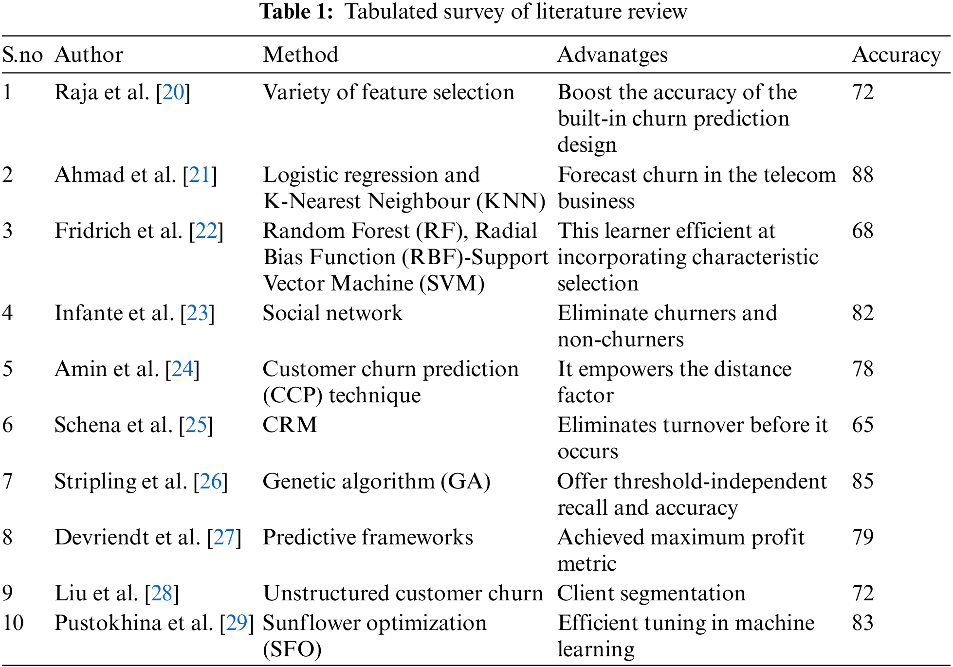
Shah et al. [9], proficient an idea to generate appropriate weights for attributes that foresee whether such a client will churn. They compared churn classifications utilized in business management, advertising, information technology, communications, newspaper articles, healthcare, and thinking. Using this strategy, various reports have studied churn damage, feature business, and forecasting models. ELM was recommended by Guang-Bin and Qin-Yu and aimed to validate a single hidden layer feedforward network (SLFN) [10]. Unlike gradient-based approaches, ELM gives random numbers to hidden layer weights and biases from the input, and these constraints are fixed throughout training [11]. Anouar [12], the author examined numerous published publications that employed ML approaches to forecast a churn in the telecommunications industry. DL approaches have shown substantial predictive power. Adadelta, Adam, AdaGrad, and AdaMax algorithms all showed improved results [13]. Recent churn prediction research exploits the time-varying nature of consumer data of Recurrent Neural Networks (RNNs) and designs such as LSTM and GRU [14]. SA has conventionally been resolved using statistical techniques (especially Cox regression, also termed proportional hazards regression) and has been used to estimate the longevity of people and products [15]. Bahnsen et al. [16], conclude that the churn ideal requires him to meet three main points. Avoid costly false positives from unnecessary bids, offer reasonable incentives to potential churners to maximize profits, and minimize the number of false positives [17]. Liu et al. [18], exhibited that using a variant of RNN like LSTM works well compared to others. The same writers also indicate that using LSTM results as a function of logistic regression(LR) yields confident results. Meta-heuristic-based feature selection is also used in customer churn prediction [19]. Table 1 indicates the recent studies of the literature survey in the churn prediction.

3  Proposed Model

Early research on churn prediction concentrated on monthly forecasts of static or dynamic churn-based behavior. The primary drawbacks of these investigations can be obscured. First off, projections of monthly churn are too late since the monthly ideal would identify customers. who clearly left early in the prior month as churn in the following month. The second issue is that taking monthly performance into account ignores variations in customer behavior from day to day during the month, which might reduce the discriminative and predictive power of the predictive model.

Thus, the goal of this work is to forecast customer churn in the daily dynamic behavior of the health insurance market. Previous models mainly focus on the monthly churn rate and it is very difficult to identify churners in advance, to overcome these difficulties, this research includes six key approaches for predicting daily customer churn constructed on day-wise client behavior. The proposed customized extreme learning machine (CELM) model shows higher accuracy than other models. Fig. 2 shows the proposed churn prediction model.

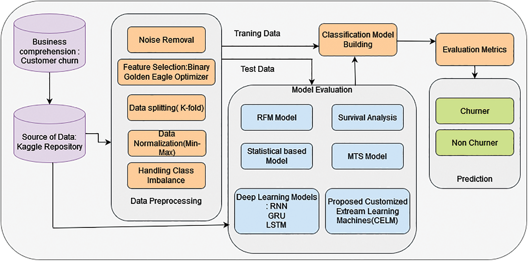
Figure 2: Proposed churn prediction model (CLEM)

3.1 Problem Statement and Dataset Description

Insurance companies competed intensely for businesses all around the globe. Due to the obvious recent increase in the highly competitive environment of health insurance businesses, clients are migrating. It’s unclear if there is evidence of switching behavior and which customers go to a competitor. When there are so many different pieces of information recorded from lots of clients, it’s hard to study and comprehend the causes of a consumer’s choice to switch insurance carriers. In an industry where client retention is similarly important, with the earliest being the costlier method, insurance companies depend on the information to evaluate client behavior to minimize loss. As a result, Our Customized Extreme Learning Machine (CELM) model will be used to investigate customer churn detection for insurance data as shown in Fig. 2 of this research. In this study, the main goal is to make an effective churn prediction system and to study the information visualization findings as thoroughly as possible. The database has been collected from the Kaggle open data website This collected database’s total size is 45,211. Dataset divided this data set into two different sets. The training set has 33,908 data points, and the test set has 11,303 data points.

3.2 Data Pre-Processing

The initial stage is to plan the dataset to realize proper input. Raw data is retrieved among all datasets in this phase, Various Data preprocessing techniques are used to transform the raw data into a useful and efficient format. Finally, valid data is supplied to the learning models.

3.3 Data Splitting (K-Fold)

Data dividing is indeed a method of dividing a database into at least 2 subgroups, referred to as ‘training’ (or ‘calibration’) and ‘testing’ (or ‘prediction’). The information that would be input into the model would be stored in the training dataset. The data used to evaluate the trained & verified strategy is contained in the testing dataset. It indicates how effective our overall model is and how frequently it would be to anticipate something that is incorrect. As mentioned above in our study, the training set consists of 33,908 data, whereas the testing set contains 11,303 data.

3.4 Binary Golden Eagle Optimizer for Feature Selection

To handle the problem of feature selection, this research uses the Binary Golden Eagle Optimizer (BGEO). In the continuous domain, the Golden Eagle Optimizer (GEO) algorithm operates. Even so, feature selection is becoming a discrete problem, so the continuous space must be transformed into a finite interval. A transfer function was used to perform the transformation. To control both exploitation and exploration, time-varying flight lengths are also suggested. As previously stated, BGEO is a good method with fewer features to tune and improved results than existing algorithms. The adaptation of binary to continuous can be given as in Eq. (1):

YNewe={0,if Randj≥U(YNewe)1,if Randj<U(YNewe)(1)

where, YNewedescribes the eth dimension for the feature position vector Y, and Randj is the random number acquired in the Jth iterative process of kind [0, 1]. Whereas if the location of the attributes j is superior to the memory place, the memory position of the attributes has been upgraded; or else, the memory remains intact. Nevertheless, the features have moved to a new location. Assume that each feature in the dataset was chosen at random [30].

3.5 RFM (Recency, Frequency, Monetary) Analysis

The RFM is a popular model in characterising client interactions and behavior overall. It is a straightforward but effective technique for computing client relationships in respect of RFM value.

1) R-Recency is the time elapsed between the consumer’s latest acquisition and the data is collected.

2) The F-Frequency of buying made by a single client within an indicated time period is made reference to.

3) The M-Monetary variable denotes the quantity of cash spent by a client over a specific time.

Definition 1. The number of steps (days) from the time interval of the last non-zero worth of Fi (ts) until t2 is defined as the Recency of Fi during specific time Window [t1, t2], for which t2-t1 = 30) Eq. (2):

R(Fi,t1,t2)=∑tst2(1)if ts<t2 else 0(2)

Definition 2. The intensity of Fi during a specific timeframe [t1, t2] is defined as (t2-t1 = 30) time scales (days) with non-zero values of Fi in Eq. (3):

(Fi,t1,t2)=∑t=t1t2(fi(t))>0(3)

Definition 3.The Monetary of Fi during such specific time window [t1, t2] is defined as the entire sum of Fi values even during [t1, t2] as in Eq. (4):

M(Fi,t1,t2)=∑t=t1t2fi(t)(4)

RFM values for every temporal feature Fi of X were mined at 2 levels.

•   Entire investigation window 30 days long.

•   Successive alternate windows of the examination window, two each 15 days long.

Therefore, the entire RFM feature direction for temp features Fi can be demarcated in Eq. (5).

RFM(Fi)=[R(Fi,1,30),Freq(Fi,1,30),M(Fi,1,30),R(Fi,t1+1,t1+30),Freq(Fi,t1+1,t2+15),M(Fi,t1+1,t1+30)]Where t1{0,15,30}(5)

When RFM actions are performed on client X in data D, a line path of 120 values is restored as relevant structures of the vendor’s temporal behaviour as during periods of statement. As a result, the transformed dataset D in Eq. (6).

D^=RFM(D)=(RFM(F11)⋯RFM(F101)⋮⋱⋮RFM(F1S)⋯RFM(F10S))(6)

The converted dataset D^ is a two-dimensional matrix, with every row representing a client and every column representing a attribute. Based on this description, the use any conventional method for binary classification to forecast churn. The research evaluated two classifiers: linear binary classifiers (LR) and non-linear binary classifiers (RF). The RF performed the best, through 100 trees and an extreme depth of 10. While the current architecture of this prototype only considers temporal characteristics, seeing static features (demographic) alongside these structures is possible.

3.6 Multivariate Time Series Construction

This process yields a set D with an MTS of size r = 10 and length m = 30, i.e., Every assessment (client) X Є D in the set comprises a 10-time series of length 30 that correlate to 10 temporal characteristic values in Eq. (7) as

D=((f11(1)⋯fr1(1)⋮⋱⋮f11(n)⋯fr1(n))(f1s(1)⋯frs(1)⋮⋱⋮f1s(n)⋯frs(n)))(7)

where fji(t) represents the rate of feature j for consumer I on time t, i = 1…s, j = 1…10, and t = 1…30. Moreover, every client X Є D in the set is considered, indicating that falls into 2 categories: churn or non-churn, indicated by 1 and 0, correspondingly. As a result, here is a label path y inEqs. (8)–(10).

y=(l1⋮ls)(8)

Where

li={1ifActivity(X.[d,d+15])=00Otherwise(9)

Activity(X,[t1,t2])=∑t=t1t2.∑j=110fji(t)>0(10)

3.7 Statistics-Based Model

Rather than RFM parameters, this model summarises each behavioral trait using various summary analyses. Minimal level, highest, mean, variance, 1st quartile, 2nd quartile (median), 3rd quartile, skewness, and kurtosis are the statistical data. For each activity type, these values are computed at two levels. This means that we'll have a vector with 36 attributes for each behavior type over the entire search window (i.e., 30 days) and every 15 days thereafter Experimented with LR and RF classifiers, and the RF classification algorithm with hundred trees and max depth = 15 performed the finest. It can be achieved by combining the fresh values with the statistical feature vector before inputting them into the RF as shown in Fig. 3.

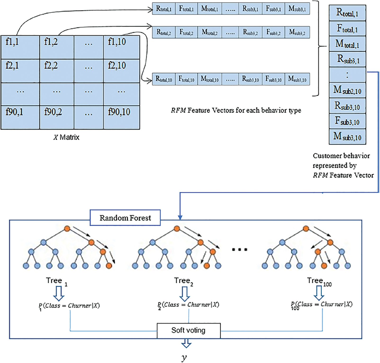
Figure 3: RFM-based model architecture

3.8 Survival Analysis

Survival analysis is a collection of techniques aimed at assessing the time to the incidence of a particular event. It is also commonly used to estimate churning error, but is applicable to virtually anything as long as you have an observation of the measured time to the event. S(t) provides the probability that a subject will survive elsewhere time t. T is a continuous variable whose cumulative distribution function (CDF) is F(t). According to Eq. (11), the survival function decreases steadily from 1 to 0 as t goes from 0 to ∞.

S(t)=Pr(T≥t)=1−F(t)=∫t∞f(x)dx0≤t<∞(11)

In overall, any spreading can be employed to denote F(t), and the suitable distribution is regularly defined by event distribution domain expertise. The incremental, Weibull, lognormal, log-logistic, gamma, and exponential-logarithmic distributions are all frequently used. In Eq. (12), the hazard function represents the error rate at which identified observations encounter events. As it increases, the rate may increase or decrease. The hazard function must meet two conditions, Eqs. (13) and (14).

λ(t)=limdt→0⁡pr(t≤T≤t+dt)dt⋅S(t)=f(t)S(t)=−S′(t)S(t)(12)

∀𝒰≥0,(λ(𝒰)≥0)(13)

∫o∞λ(𝒰)d𝒰=∞(14)

The default distribution is represented by the cumulative hazard function, which can be represented in Eq. (15). It is a function that does not decrease.

∧(t)=∫0tλ(𝒰)d𝒰(15)

Parts of Eqs. (11) and (12) can be used to derive a convenient method for the survival function and hazard rate.

λ(t)=f(t)S(t)=−S′(t)S(t)=−ddtlog⁡S(t)(16)

S(t)=exp{−∫0tλ(𝒰)d𝒰}=exp{{−∧(t)}∧(t)}(17)

Churn prediction could be viewed as a component of SA. In churn forecast, time it is constant, and the primary objective is to decide whether or not the subject continues to leave earlier time t, which conforms to the definition of the equation. Eqs. (16) and (17) show S(t). In this light, churn can be designed as a binary classification problem.

The Kaplan-Meier modeller is a non-parametric estimate of the survival analysis function developed by Kaplan and Meier in 1958. Eq. (18) explains the function, which yields a slope that is true to the actual survival function by accumulating estimations over t. Here, ti indicates the ordered time points following as a minimum one event, di indicates the number of occurrences, and ni indicates the residual examples that have not yet experienced the event in Eq. (18).

S^(t)=∏i:ti<t(1−dini)(18)

3.9 Recurrent Neural Networks

RNN allows the formation of cycles among hidden units. This allows the RNN to retain the inner state memory of earlier inputs, making it suitable for modelling sequential data [31]. Sequential forecasts in RNNs are shaped by iterative inputs of the network output at each time step. To simplify gradient computation during backpropagation, recurrent neural networks should be unrolled into directed acyclic graphs. when training the network, then network can use the standard learning methods used in regular feedforward architectures. The unfolded architecture reveals that the states of hidden units are affected by previous ones.

3.10 Long Short-Term Memory

LSTM architectures, developed by Hochreiter and Schmidhuber in 1997, are designed to learn long-term dependencies, allowing them to retain memory for extended periods of the period than classic RNNs. The distinction is in his LSTM cells. LSTM cells have some extra components and a more complex structure, which includes forget gates, input gates, and output gates. There are also cell state and hidden state that is modernized after each gate. The gate controls which facts are forgotten, the input gate controls the importance of the value to acquaint, and the output gate modernizes the cell's hidden layer.

3.11 Gated Recurrent Unit

The framework of the GRU cell is very related to that of the LSTM. There are only two aspects inside the GRU cell: the reset and update gates. The reset gate determines what data to forget and what data to add, whereas the reset gate influences what previous data to forget. In contrast to the LSTM cell, GRU does not have a cell state and instead employs the hidden state for identical determination. Training times are usually faster than LSTM due to its simpler structure.

3.12 Extreme Learning Machine

ELM is a single-layer feed-forward neural network learning method (SLFN). The ELM model delivers excellent results at extremely fast learning speeds. The ELM does not employ a gradient-based method, unlike classical feedforward network learning algorithms such as the Back-propagation (BP) method shown in Fig. 4. All parameters are adjusted only once with this technique. Iterative training is not required for this algorithm.

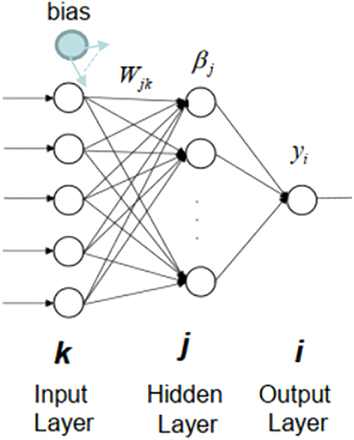
Figure 4: Extreme learning machine model

1. Generate the input layer’s random weights matrix and bias. The weight matrix and bias have the dimensions (j x k) and (1 x k), correspondingly, where j is the no of hidden nodes and k is the no of input nodes in Eq. (19) as

W=[rand⋯rand⋮⋱⋮rand⋯rand](19)

2. Determine the hidden layer output vector. By multiplying X, which represents training data, by the transposed weight matrix, the original hidden layer output grid is determined in Eq. (20) as.

Hinit=X⋅WT(20)

3. Select an activation function. You can select any activation function you would like. However, in this example, I will use the function for sigmoid activation because it is simple to implement in Eq. (21) as

H=11+e−Hinit(21)

4. Determine the Moore-Penrose pseudoinverse. There are several methods for calculating the Moore-Penrose generalised inverse of H. Orthogonal extrapolation, orthogonalization method, variational iteration method, and decomposition of singular values are examples of these methods (SVD) in Eqs. (22) to (24).

H+=(HT.H)−1.HT(22)

5. Compute the output weight matrix beta

β^=H+.Y(23)

6. Step 2 should be reiterated for the testing set, creating a fresh H matrix.

Generate an outcome matrix named ŷ after that. To employ the well-known beta matrix.

Y^=H.β^(24)

All parameters are adjusted only once due to non-iterative training. This results in a rapid training rate. Its employment is simple to grasp and can be used to answer difficult problems. As a result, ELM drastically reduces working time and converts the unique nonlinear training problem into linear training troubles. Fig. 5 containing Activation functions in ELM:

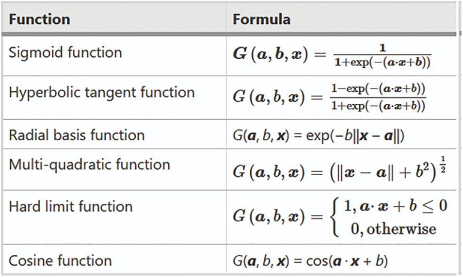
Figure 5: Activation functions in ELM

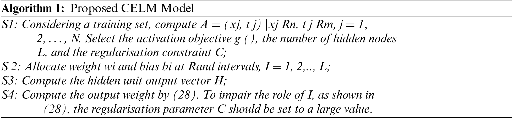
3.13 Proposed Customized Extreme Learning Machines

As per statistical learning, a learning model’s actual forecast risk is split into two components, structural risk (SR) and empirical error (ER). Considering, training ELMs with constant optimizers reduces only the ER, not the SR. The Customized word is presented in the previous ELMs to establish the Customized extreme learning machine to reduce structural risk. The less SR will improve the prediction rate of the learning model is shown in Figs. 6 and 7 are represented in Eqs. (25) to (28).

min12∥β∥2+C2∥ε∥2(25)

Here C is the regularisation constraint, and the terms ∥ε∥2 (resp. ∥ε∥2) are associated with empirical (resp. structural) risk. Its Lagrangian Eq. (26) is as follows:

L(α,ε,β)=12∥β∥2+C2∥ε∥2−α(Hβ−T−ε)(26)

Here R = (1, 2,…, N) denotes the operator. Starting to take the half results with respect to α, ε and β to

{dLdβ=0→βT=αHdLdε=0→α=CεdLdε=0→Hβ−T−ε=0(27)

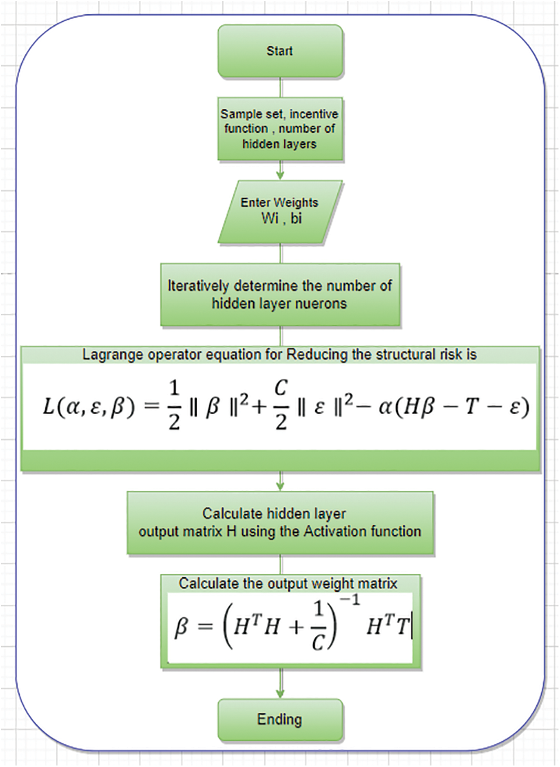
Figure 6: Flow chart of Proposed CELM

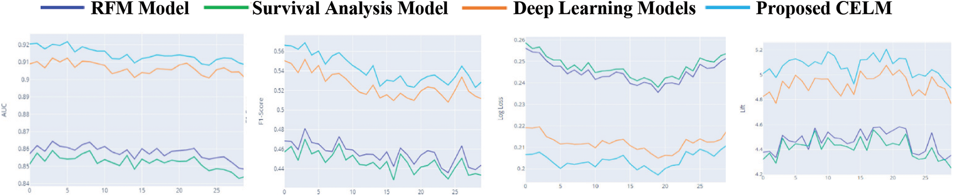
Figure 7: Performance of top 4 models with respect to metrics

The output weight matrix is then obtained.

β=(HTH+1C)−1HTT(28)

Where I denote the identity matrix

4  Experimental Results

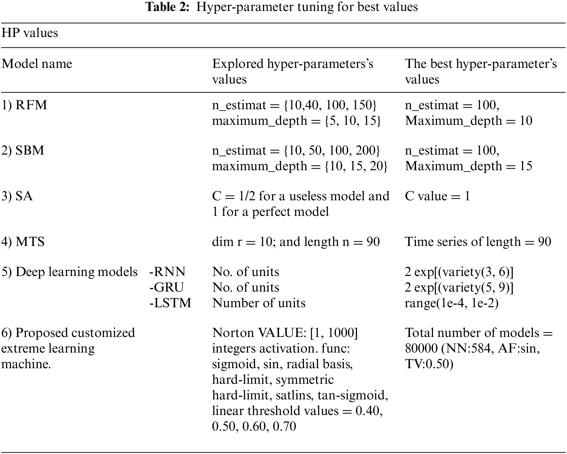
In this study, the research focussed on our experimental studies for endorsing the suggested everyday churn prediction models and trying to compare them to the different daily and monthly churn prediction approaches described in Section 2. Our concepts are specifically compared to the following approaches. Five measures were used for model evaluation and comparison: Area Under the Curve(AUC), log loss, accuracy, and F1 score. Furthermore, Lift denotes the churn rate with the highest predicted probability of 10% over the actual client base churn rate, and the Expected Maximum Profit Measure of the Churn rate (EMPC). The AUC has measured a more common metric as it précises the whole enactment with all possible limits. The EMPC is a new performance metric specifically planned to measure the performance of churn forecast methods given the cost and expected return of customer retaining campaigns. Default constraint values (α = 6; β = 14; CLV = 200; d = 10; f = 1) were used to calculate the EMPC metric. Tune the model hyper-parameters to fit the grid search method. Hyper-parameter space and optimal values These constraints for each model are shown in Table 2.

The mean and SD values for the five metrics of the model within the test forecast window are shown in Tables 4 and 5. Furthermore, Table 6 shows the model's average rank and average overall rank as computed by the five performance measures. To check the generalizability of the model, the research also shows the values of the measurements on the validation set. Graphical information of mean, standard deviation, and average ranks of all parameters are shown in Figs. 7–10. The AUC graph of performance metrics is shown in the below figures. This evaluation will take into account four factors: True Positive, True Negative, False Positive, and False Negative. Table 3 represents the comparison of different parameters. The confusion matrix of the testing set for the churn prediction is specified as follows in Table 3.

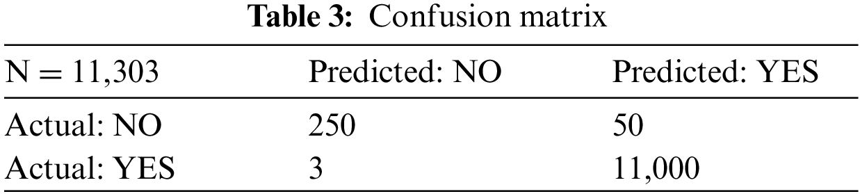
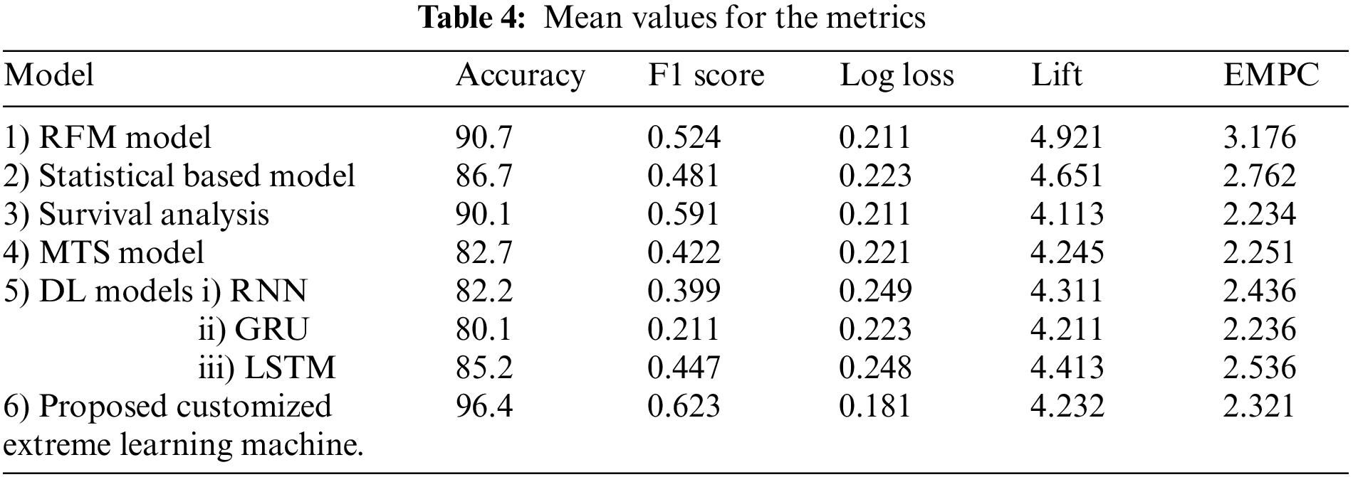
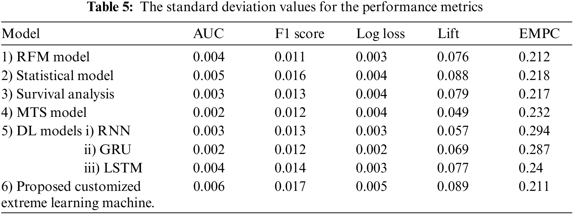
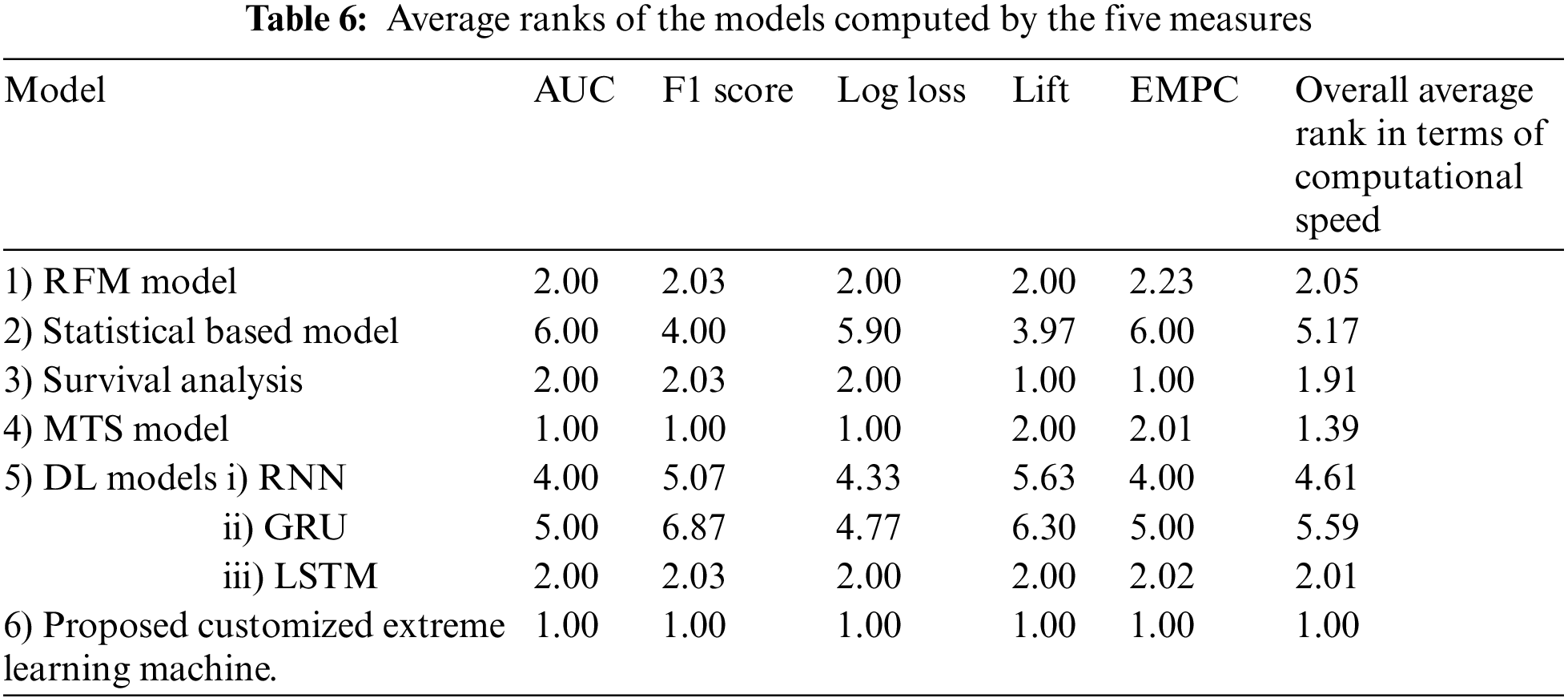
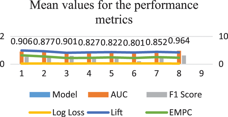
Figure 8: Mean values graph for the Metrics

Figure 9: The SD values for the metrics

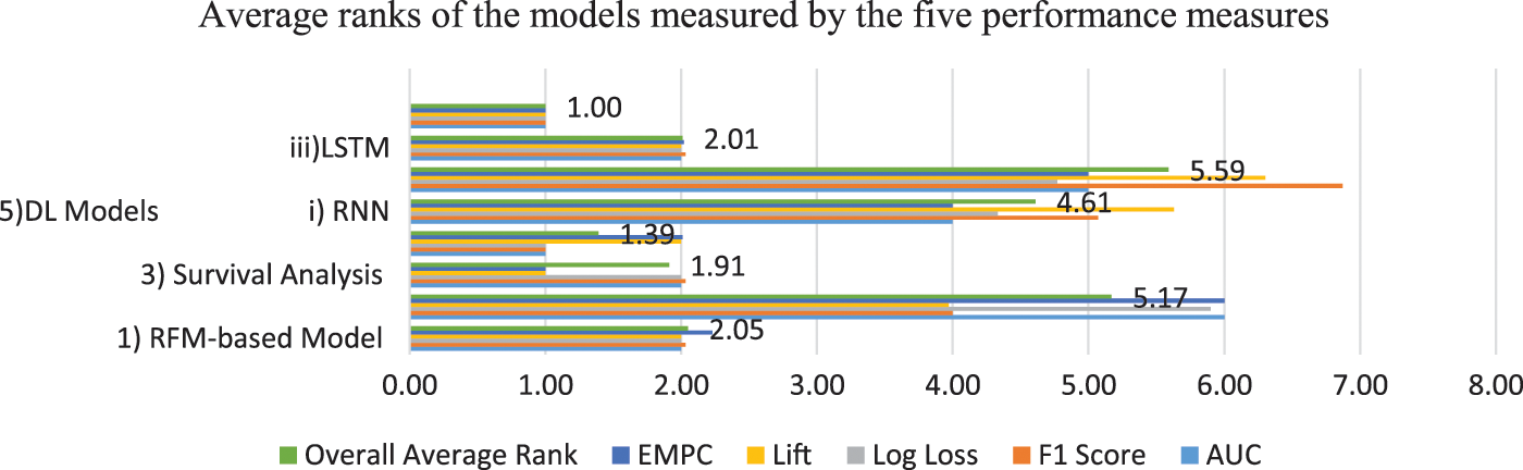
Figure 10: Avarage ranks of the models measured using all performance metrics

As shown in Fig. 11, the original RFM model of customer distribution has two subgroups each containing a dominant type, plus a smaller subgroup containing both types (churners and Non–Churners ). The multivariate time series separated several churners in one region (a leftmost region in Fig. 12). Statistical expressions are nonlinearly separable. The survival analysis models in Figs. 13 and 14 shows that a nonlinear classifier is required to get good predictions. In contrast, deep learning models show the clearest separation between those who are willing to churn and those who are not, as Fig. 15 shows. Fig. 16 displays the classification of churners and non-churners by the proposed CELM model.

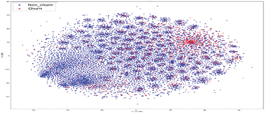
Figure 11: RFM model churners and non–churners

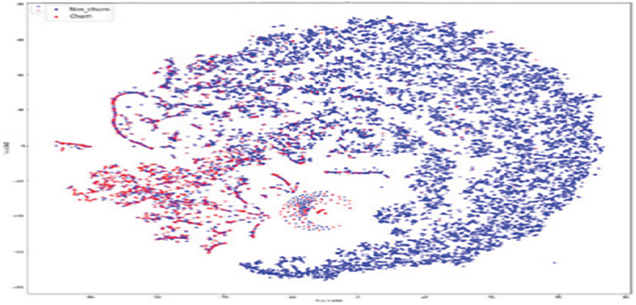
Figure 12: MTS model for churners and non–churners

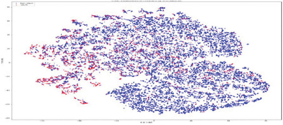
Figure 13: SM model for churners and non–churners

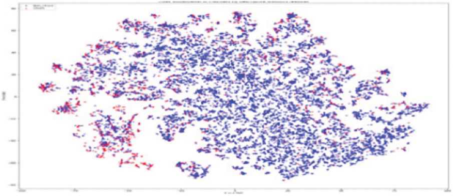
Figure 14: SA model for churners and non–churners

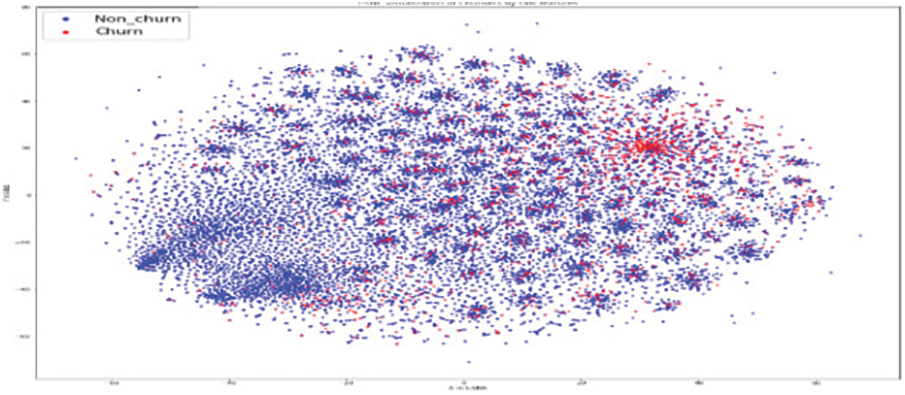
Figure 15: LSTM model for churners and non–churners

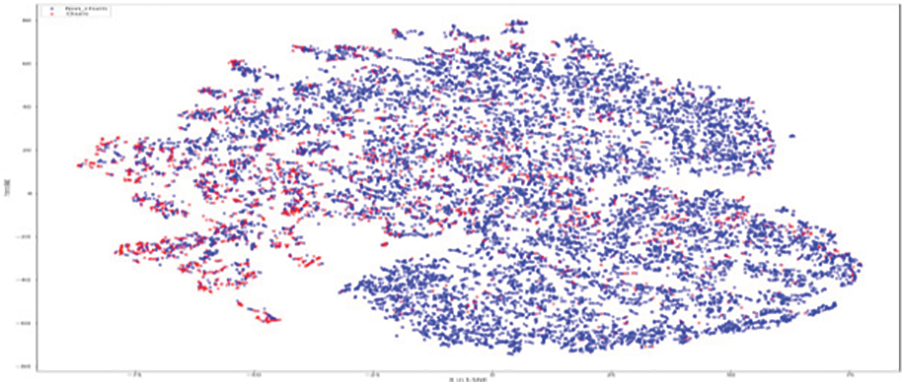
Figure 16: Proposed CELM for Churners and non–churners

First, a t-Stochastic Neighbour Embedding (t-SNE) method, is used to visualize the raw illustration of the customers, which consisted of 20 K row vectors with 900 values each. Fig. 9 depicts the result. The output of the final hidden units (fully connected layer with 128 neurons) in the LSTM model is gone to t-SNE to visualize the required learners by RFM and SA designs. The related outputs are displayed in Figs. 11 and 12. The RFM feature set of 120 values/the statistical data feature vector of 360 values was passed to the t-SNE for visualization of the SM representation. Figs. 13 and 14 display the output of the RFM illustration and the statistics depiction, respectively. As illustrated in Fig. 15, the major factor of clients has small subsets that include both kinds (churners and non-churners), as well as two subsets that each consist of one dominant type.SA has separated some churners in one neighbourhood (the most left area of Fig. 13). CELM has the best and most accurate split of churners and non-churners as shown in Fig. 16.

5  Conclusion

Studies that considered static churn modelling centered on forecasting churn on a monthly basis. Previous investigations, as stated in the literature section is aimed at churn as a static prediction issue. The research goal in this manuscript is to forecast churn on a daily basis based on dynamic variations in customer behavior. In this way, clients who are prone to churn can be identified in advance, and the maintenance cost of client management can be reduced accordingly. As a result, the research denoted the customer’s daily behavior using six different approaches and used this representation to formulate the problem of daily churn prediction. The findings demonstrate that the proposed model CELM, is more accurate than monthly techniques in operationally forecasting churners’ advances. This is critical from a business standpoint in order to improve the effectiveness of retention advertising campaigns. Furthermore, the research discovered that the frequency of the input is the first contributor to prediction accuracy, with daily behavior being preferable to monthly behavior. Along with the retention effect, there are a number of significant aspects that future research may take into account. The model lacks the causality necessary for trying to target and can be used to develop a straightforward daily churn prediction model, but more work is required for interpretability. Because the results are comprehensible, industries can interpret them. Based on their reasons for departing, target your churning customers. The model might be an LSTM with attention-based learning. The second problem has to do with the inaccurate churn prediction caused by targeting. This suggests that it is insufficient to simply identify consumers at a high risk of leaving. Determine how to target customers for your business based on how they respond to retention tactics.

Funding Statement: The authors received no specific funding for this study.

Conflicts of Interest: The authors declare that they have no conflicts of interest to report regarding the present study.

References

1. P. Granberg, “Churn prediction using time series data (Dissertation),”Digitala Vetenskapliga Arkivet, vol. 931, no. 3, TRITA-EECS-EX,2020. [Google Scholar]
2. D. Yumo, E. W. Frees, F. Huang and K. C. H. Fransis, “Multi-state modelling of customer churn,” ASTIN Bulletin: The Journal of the IAA, vol. 52, no. 3, pp. 735–764, 2022. [Google Scholar]
3. https://www.zendesk.com/in/blog/customer-churn-rate/. [Google Scholar]
4. N. Alboukaey, A. Joukhadar and N. Ghneim, “Dynamic behavior based churn prediction in mobile telecom,” Expert Systems with Applications, vol. 162, no. 2, pp. 113779, 2020. [Google Scholar]
5. M. Óskarsdóttir, T.year VanCalster, B. Baesens and W. Lemahieu, “Time series for early churn detection: Using similarity based classification for dynamic networks,” Expert Systems with Applications, vol. 106, pp. 55–65, 2018. [Google Scholar]
6. S. Sathe and C. Aggarwyearal, “Similarity forests,” in Proc. of the 23rd ACM SIGKDD, Int. Conf. on Knowledge Discovery and Data Mining, Halifax, NS, Canada, pp. 395–403, 2017. [Google Scholar]
7. T. Vafeiadis, K. I. Diamantaras, G. Sarigiannidis et al., “A comparison of machine learning techniques for customer churn prediction,” Simulation Modelling Practice and Theory, vol. 55, pp. 1–9, 2015. [Google Scholar]
8. Y. Qu, Y. Fang and F. Yan, “Feature selection algorithm based on association rules,” in Journal of Physics: Conference Series. Vol. 1168. Beijing, China: IOP Publishing, pp. 52012, 2019. [Google Scholar]
9. M. Shah, A. Darshan, B. Shabir and V. Viveka, “Prediction and Causality analysis of churn using deep learning,” Computer Science and Information Technology, vol. 9, no. 13, pp. 153–165, 2019. [Google Scholar]
10. B. G. Huang, Q. Y. Zhu and S. CheeKheong, “Extreme learning machine: Theory and applications,” Neurocomputing, vol. 70, no. 3, pp. 489–501, 2006. [Google Scholar]
11. A. Spooner, E. Chen, A. Sowmya, P. Sachdev, N. A. Kochan et al., “A comparison of machine learning methods for survival analysis of high-dimensional clinical data for dementia prediction,” Scintific Reports, vol. 10, no. 1, pp. 20410, 2020. [Google Scholar]
12. D. Anouar, “Impact of hyperparameters on deep learning model for customer churn prediction in telecommunication sector,” Mathematical Problems in Engineering. vol. 2022, pp. 11, 2022. [Google Scholar]
13. Ahn. Jaehyun, J. Hwang, D. Kim, H. Choi and S. Kang, “A survey on churn analysis in various business domains,” IEEE Access, vol. 8, pp. 220816–220839, 2020. [Google Scholar]
14. G. Mena, A. DeCaigny, K. Coussement, K. W. DeBock and S. Lessmann, “Churn prediction with sequential data and deep neural networks a comparative analysis,” arXiv: 1909.11114v1 [stat.AP], 2019. [Google Scholar]
15. P. Wang, L. Yan and C. K. Reddy, “Machine learning for survival analysis: A survey,” ACM Computing Surveys (CSUR), vol. 51, no. 6, pp. 1–36, 2016. [Google Scholar]
16. A. C. Bahnsen, A. Djamila and B. Ottersten, “A novel cost-sensitive framework for customer churn predictive modeling,” Decision Analytics, vol. 2, no. 1, pp. 1–15, 2015. [Google Scholar]
17. K. Naimisha and N. Balakrishnan, “Hybrid features for churn prediction in mobile telecom networks with data constraints,” in 2020 IEEE/ACM Int. Conf. on Advances in Social Networks Analysis and Mining (ASONAM), Long Beach, CA, USA: IEEE, pp. 734–741, 2020. [Google Scholar]
18. L. Rencheng, A. Saqib, S. Fakhar Bilal, Z. Sakhawat, A. Imran et al., “An Intelligent hybrid scheme for customer churn prediction integrating clustering and classification algorithms,” Applied Sciences, vol. 12, no. 18, pp. 9355, 2022. [Google Scholar]
19. J. Nagaraju and J. Vijaya, “Boost customer churn prediction in the insurance industry using meta-heuristic models,” International Journal of Information Technology, vol. 14, no. 5, pp. 2619–2631, 2022. [Google Scholar]
20. J. Beschi Raja, G. Sandhya, S. Sam Peter, R. Karthik and F. Femila, “Exploring effective feature selection methods for telecom churn prediction,” International Journal of Innovation Technology Exploration. Engineering. (IJITEE), vol. 9, no. 3, pp. 620, 2020. [Google Scholar]
21. K. Abdelrahim Ahmad, A. Jafar and K. Aljoumaa, “Customer churn prediction in telecom using machine learning in big data platform,” Journal of Big Data, vol. 6, no. 1, pp. 1–24, 2019. [Google Scholar]
22. Fridrich and martin, “Explanatory variable selection with balanced clustering in customer churn prediction,” Ad Alta: Journal of Interdisciplinary Research, vol. 9, no. 1, pp. 56–66, 2019. [Google Scholar]
23. C. Infante, L. Óskarsdóttir and B. Baesens, “Evaluation of customer behavior with temporal centrality metrics for churn prediction of prepaid contracts,” Expert Systems with Applications, vol. 160, pp. 113553, 2020. [Google Scholar]
24. A. Amin, A. Obeidat, F. Shah, B. Adnan, A. Loo et al., “Customer churn prediction in telecommunication Industry using data certainty,” Journal of Business Research, vol. 94, no. 94, pp. 290– 301, 2019. [Google Scholar]
25. F. Schena, “Predicting customer churn in the insurance industry: A data mining case Study,” in Rediscovering the Essentiality of Marketing, vol. 2, pp. 747–751, Chem, UAE: Springer, 2016. [Google Scholar]
26. E. Stripling, V. Broucke, S. Antonio, K. Baesens, M. Snoeck et al., “Profit maximizing logistic model for customer churn prediction using genetic algorithms,” Swarm and Evolutionary Computation, vol. 40, no. 3, pp. 116–130, 2018. [Google Scholar]
27. F. Devriendt, J. Berrevoets and W. Verbeke, “Why you should stop predicting customer churn and start using uplift models,” Information Sciences, vol. 548, no. 1, pp. 497–515, 2021. [Google Scholar]
28. S. Liu, X. Li and G. Xu, “Leveraging unstructured call log data for customer churn prediction,” Knowledge-Based Systems, vol. 212, pp. 106586, 2021. [Google Scholar]
29. I. V. Pustokhin, D. A. Pustokhin, R. H. Aswathy and T. Shankar, “Dynamic customer churn prediction strategy for business intelligence using text analytics with evolutionary optimization algorithms,” Information Processing & Management, vol. 58, no. ,6, pp. 102706, 2021. [Google Scholar]
30. R. K. Eluri and N. Devarakonda, “Binary golden eagle optimizer with time-varying flight length for feature selection,” Knowledge-Based Systems, vol. 221, no. 247, pp. 108771, 2022. [Google Scholar]
31. J. Nagaraju and J. Vijaya, “Methodologies used for customer churn detection in customer relationship management,” in Int. Conf. on Technological Advancements and Innovations(ICTAI), Tashkent, Uzbekistan, pp. 333–339, 2021. [Google Scholar]
Cite This Article
Copyright © 2023 The Author(s). Published by Tech Science Press.
This work is licensed under a Creative Commons Attribution 4.0 International License , which permits unrestricted use, distribution, and reproduction in any medium, provided the original work is properly cited.
Downloads
Citation Tools