Video Frame Prediction by Joint Optimization of Direct Frame Synthesis and Optical-Flow Estimation

1  Introduction

Next-frame prediction is the problem of generating future frames by adopting the spatiotemporal correlation between a given set of current and past successive frames. Such predictive cognitive neural networks are often considered the essence of computer vision. They play a critical role in a variety of applications, such as abnormal event detection [1], autonomous driving [2–4], intention prediction in robotics [5,6], video coding [7,8], collision avoidance systems [9,10], activity and event prediction [11,12], and pedestrian and traffic prediction [13–15]. However, modeling future image content and object motion is challenging due to dynamic evolution and image complexity, such as occlusions, camera movements, and illumination. In the past, statistical algorithms such as Hidden Markov Model [16,17], Dynamic Random Forests [18], Gaussian Mixture Model [19], and Boltzmann Machine [20] have been used for simple periodic motion. On the other hand, data-driven approaches with Deep Learning were considered, for more complex scene evolutions.

Recently, the Deep Neural Network model has become popular in various fields because of its ability to handle multidimensional data without feature engineering, nonlinear learning capabilities, and availability of cheap and high computational power [21–24]. Numerous attempts have been made for frame prediction with Deep Learning in the past. The top-performing algorithm exploits spatiotemporal feature learning in an unsupervised manner without the need for labeled data. They are designed to take advantage of supervised learning by generating infinite training samples for input-output, where the predicting frame (output label) is taken from the database. In general, these models either learn to compute optical flow (motion) on a pixel-by-pixel basis or learn to synthesize RGB pixels by finding correspondences between given frames. These predictive models are generally based on autoencoder [25,26], (where the models first learn spatiotemporal features by encoding multiple input images into a small latent state and later reconstruct them to predict the future image with small reconstruction error), recurrent neural networks [27,28], (where the model directly learns the temporal correlations between input frames, to predict the future frame) or generative adversarial networks [29–31] (where two neural networks compete with each other, among them generative network predicts future frame based on the past observed frames, while the discriminative network classifies the output image as real or fake). These models have significant drawbacks. In the pixel-based motion approach, the model is prone to errors in extrapolating the future frame due to lighting conditions, object occlusion, and camera movements. With RGB synthesis, it is difficult to estimate all content and object motion in the scene, often resulting in blurry prediction.

Inspired by the successful application of Convolutional Autoencoder [32,33] and Long Short-Term Memory (LSTM) [34]. In this work, we propose a deep Frame Prediction Network (FPNet-OF) with a multi-prediction branch (Optical flow and Frame) for predicting future images, as shown in Fig. 1. We developed the ‘Frame Prediction Branch’ based on a recurrent convolutional autoencoder architecture [14] to learn the spatiotemporal correlation for a given past frame to predict the future frames. However, the frame-based architecture alone doesn’t generate a coherent image (as shown in the ablation study in Section 4.4.1), as the relationship between objects motion in subsequent frames are not unique. Moreover, the predicted image becomes blurred or fuzzy when the prediction range is several time-steps in the future. Therefore, we design a second convolutional autoencoder (optical-flow prediction branch) in parallel with the frame prediction branch, which is identical to the frame prediction branch and learns to incorporate future object motion, as shown in Fig. 1. The optical-flow prediction branch is connected through element-wise multiplication operations at the decoder module of the frame prediction branch. The input to optical-flow architecture is the sequence of past optical-flow images (optical-flow image is generated from the corresponding original frames, explained in Section 4.2). A detailed explanation of the architecture design is presented in Section 3.2 and the training process in Section 3.3. The main contribution of the paper is summarized as follows:

•   We proposed a deep neural prediction network, FPNet-OF, made of two identical branches named frame prediction branch and optical-flow prediction branch to predict the future video frame. The branches are made up of the recurrent convolutional autoencoder architecture. These branches exploit the spatio-temporal relation of the past image sequences to learn future representations. The frame prediction branch takes past frames to generate the future frame. The optical-flow prediction branch takes past optical-flow images to synthesize the future optical flow images.

•   We adaptively fuse future optical-flow estimation (from optical-flow prediction network) to reconstruction layer of frame prediction network, using an element-wise multiplication layers. This enables frame prediction network to adjust the magnitude range of moving object, benefiting high-quality future prediction.

•   Exhaustive experiments validate that the FPNet-OF demonstrate a state-of-the-art performance in terms of Structural Similarity Index (SSIM), peak signal-to-noise ratio (PSNR), and mean square error (MSE) on Caltech, UCF101, CUHK Avenue, and ShanghaiTech Campus datasets.

Figure 1: FPNet-OF model architecture, made up of frame prediction branch and optical-flow prediction branch. Each branch further made up of three modules, section A and D are encoder module, Section B and E are recurrent network, and section C and F are decoder module. The color code represents the type of operations

In this section, we describe the background and motivation of the study. The rest of the paper is structured as follows: Section 2 discusses related works. Section 3 presents the methodology, including problem statements, key components of FPNet-OF architecture design, the loss functions, and the training process. Section 4 presents the data source, optical-flow generation from frame image, model implementation details, model performance, and comparison with other state-of-the-art models. Finally, Section 5 concludes our work and provides the future direction of this study.

2  Related Works

In many computer vision applications, it is important to correctly predict future scenarios to avoid undesirable outcomes. In this study, we aim to predict the future frames by incorporating the future optical-flow motion into the direct RGB synthesis. This is in contrast to most recent work, where researchers mainly focused on developing a neural network architecture by using either direct frame synthesis or optical-flow motion. Here, we jointly optimize direct RGB frame prediction and future dense optical motion estimation to develop a superior prediction network. In the following subsections, we will discuss in detail the most relevant work for our study.

2.1 Direct Frame Synthesis

The direct frame synthesis approach exploits spatiotemporal information in numerous ways that depend on the design of the network architecture. Some of the common approaches [35–43] are based on 3D convolutional neural networks (3D-CNN), convolutional autoencoder, recurrent networks, and generative adversarial training methods. The 3D-CNN-based model learns spatiotemporal features as it performs convolution operations across temporal and spatial dimensions. In [44] researchers used 3D-CNN with the input of a short clip to predict the temporal motion in the video. The limitation of 3D-CNN is that it only considers short-term dependencies and cannot model the learning of long-term features. To overcome this limitation, most of the existing work uses the hybrid architecture of convolutional networks and recurrent networks, which allows to simultaneously exploit the convolutional model’s ability to learn spatial relationships and the recurrent model’s ability to capture temporal relationships. In [39], the researcher proposes an action-dependent video prediction model using two spatiotemporal prediction architectures based on convolutional networks and recurrent neural networks to directly control one or more objects in Atari games by action and indirectly influence many other objects. Finn et al. [45] proposed an action-based video prediction model based on Convolutional LSTMs to explicitly make a long-range prediction in real videos by predicting a distribution over pixel motion from previous frames. Yu et al. [35] use a hybrid network based on a 3D convolution and recurrent network to build a two-way autoencoder for predicting future frames by spatiotemporal learning. Ranzato et al. [40] propose a recurrent convolutional neural network to handle spatial correlations between nearby image patches. The model leverages both temporal dependencies and spatial correlations to predict the central patch of missing frames or extrapolate future frames from an input video sequence. Lotter et al. [46] introduced a predictive neural network based on the CNN-LSTM-deCNN frame to predict future images and learn the latent structural representations of the three-dimensional objects in a synthetic video sequence. Lotter et al. [8] proposed a predictive neural network (PredNet) based on ConvLSTM inspired by the concept of “predictive coding” to predict future frames in a video sequence by making a local prediction in each layer and passing only the deviation of the prediction to the subsequent layers.

Although the aforementioned works make a significant contribution to video prediction, these works often lead to blurry predictions. In [38], the author proposes a multi-scale architecture with an adversarial training process and a new loss function based on the image gradient to cope with the inherently blurry predictions obtained with the standard loss function mean squared error. Byeon et al. [47] identified blind spots (lack of access to all relevant past information) as an important factor for blurry prediction and propose a fully context-aware video prediction (ContextVP) that captures all available context for each pixel using parallel multidimensional LSTM units and aggregates them using blending units. Kwon et al. [31] propose a unified generative adversarial network with a single generator and two discriminators (to identify fake frame and fake contained image sequences from the real sequence) that can predict both future and past frames enforcing bi-directional prediction consistency using retrospective cycle constraints.

2.2 Optical Flow Estimation

Optical flow is the most commonly investigated method for predicting future motion fields or video frames [25,48,49] and the quality of the prediction depends on the accuracy of the flow generation for a given image or video sequence. In general, large displacements or the fast motions in the video clips poses problems. Mahajan et al. [50] describe an image interpolation technique for generating a sequence of intermediate frames by simply copying and moving pixel gradients from the input images along the path. Luo et al. [51] present an unsupervised learning approach that compactly encodes the motion dependencies in video clips to predict the long-term 3D motions based on the LSTM Encoder-Decoder framework. Since the work by Horn et al. [52], optical flow estimation has been dominated by variational methods [25,49]. Revaud et al. [49] propose EpicFlow, a novel approach for estimating optical flow in presence of large displacements and significant occlusions through a sparse-to-dense interpolation scheme of correspondences based on edge-aware distance. Dosovitskiy et al. [53] propose FlowNet, which is based on CNN’s and capable of solving optical flow estimation problems by correlating the feature vectors at different image positions. Liu et al. [26] propose Deep Voxel Flow (DVF), a deep network that learns to synthesize video frames by flowing pixel values from previous frames.

2.3 Joint Frame Prediction and Optical Estimation

More recently, researchers have focused on developing a hybrid deep neural network that takes advantage of both optical-flow estimation and direct RGB frame synthesis for the task of video prediction [1,54–56]. Sedaghat et al. [56] propose NextFlow trained in a semi-supervised hybrid multitasking environment to use real-world videos without ground truth and synthetic images with ground truth to learn optical flow estimation and next frame prediction. Lui et al. [1] propose a video prediction framework for anomaly detection, to predict a high-quality future frame for normal events, a motion (temporal) constraint-based on optical flow is introduced in addition to appearance (spatial) constraints on intensity and gradient. The spatial and temporal constraints predict future frames for normal events and consider events as abnormal if the event does not confirm the expectation. Liang et al. [54] proposed Dual Motion GAN, which learns to explicitly enforce the prediction of the future frame to be consistent with the pixel-wise flows in the video sequence through a dual learning mechanism. Li et al. [55] proposed a deep multi-branch mask network (DMMNet) that adaptively combines the advantages of optical-flow wrapping and RGB pixel synthesis to predict video frames.

Although direct frame synthesis and optical flow estimation provide compelling results, they often reach their limits. In particular, direct frame synthesis often leads to fuzz prediction because these models cannot explicitly model complex pixel distributions, and the image becomes blurrier or fuzzier when the prediction range is several time steps in the future. On the other hand, optical-flow estimation is poor in situations with large displacements, distortions, motions, and obstructions and produces significant artifacts due to inaccurate flow estimation. In the case of research focused on joint frame prediction and optical-flow estimation, these methods are comparatively better than individual system but with further room for improvement, they are tough to train due to their sizeable network architecture. Initially, our model has longer training time per epoch, as it trains both the Frame Prediction Branch and the Optical-flow Prediction Branch simultaneously. As the optical-flow images have lower pixel distribution complexity than the original frames, the Optical-flow Prediction Branch requires fewer epochs to train than the Frame Prediction Branch. When the Optical-flow Prediction Branch starts to predict the accurate future optical-flow, we halt the training of the Optical-flow Prediction Branch, resulting in the decrease of the overall training time of the model per epochs. Hence, the FPNet-OF is a lightweight architecture and easier to train. Moreover, in contrast to the work in [55], where the researcher fuses the future motion and future appearance synthesis only at the last layer. Here in this work, the future motion of the optical flow from the Optical-flow Prediction Branch merges with the Frame Prediction Branch at different depths, supplementing the advantage of both architecture to achieve more realistic results.

3  The Proposed Method

In this section, at first, we define the problem statement for the next frame prediction. Secondly, we elaborate on all the modules of the proposed FPNet-OF model in detail. Finally, we present the objective function and model training process.

3.1 Problem Statement

Let F∈{f0,f1,f2,…,fn−1} be the chronological order of n original-frame images and O∈{o1,o2,…,oi,…,on−1} be the chronological order of n−1 optical flow image, such that ith optical flow ‘oi’ is generated from frames  { fi−1,fi}∈F. We proposed a deep neural network (ℱ) which takes input (X) list of past p consecutive frames and optical flow to predict output  (Y)  which is   kth future frame  fp+k. We denote our prediction frame as  f^p+k. To make f^p+k close to  fp+k, we minimize their distance regrading intensity, gradient and structure similarity. Table 1 shows the input sequence and its corresponding prediction frame for 1st  and  ith  samples.

Ypi=ℱ(Xpi,θ)(1)

Here, θ  is the model parameter.

Here, X⋅ represent the sample number and X⋅ represent the number of past consecutive images. The model M can be defined as

3.2 Model Architecture

As mentioned earlier, FPNet-OF contains two branches: Frame Prediction Branch and Optical-flow Prediction Branch. Each branch is composed of three modules: (i) Encoder Module (feature extraction network), which extracts features from the input by gradually reducing the spatial resolution; (ii) Recurrent Module (recurrent network), which learns the spatial and temporal features; and (iii) Decoder Module (reconstruction network), which gradually recovers the frame by expanding the spatial resolution. Both branches consist of multiple skip connections from their respective encoder module to the decoder module. The architecture of both branches is identical, except that the decoder module in the frame prediction branch has an additional connection (optical-flow connection) from the decoder module of the optical-flow prediction branch. A schematic of our framework is shown in Fig. 1.

3.2.1 Feature Extraction Network

The encoder module consists of an input layer followed by series of four encoder blocks stacked on top of each other. Each encoder block consists of one Pooling Block (PB) to achieve shift-invariance by gradually reducing the spatial resolution of the feature map while learning important information, followed by a Convolutional Residual Block for spatial receptive learning. Residual learning is used in the Convolutional Residual Block to overcome a degradation problem (a condition in which the accuracy of a deep neural network enters saturates at one point and then rapidly degrades). The degradation problem often occurs in networks with high depth, as reported in [57]. Deep residual learning was first introduced in [57] to overcome the degradation problem, and the application of residual learning can be seen in [58]. Unlike traditional neural networks where the layer feeds to the next layer, in residual learning, the current layer feeds into the next layer and also feeds to the layers about few hops away. The residual block makes use of shallow features to get more key features.

In our proposed architecture, Convolutional Residual Block is made by stacking two CNN blocks. Each CNN block consists of a 2D Convolutional layer with the strides of 1×1 and filter kernel size of 3×3, followed by a Batch Normalization layer, and a ReLU activation layer. We adopt the Convolutional Residual block as seen in Fig. 2a. The output of CNN block 1 is directly fed to CNN block 2. The result from the batch normalization layer of the CNN block 2 is first element-wise added with the input of Convolutional Residual block (performed by shortcut connection) and then passed through ReLU nonlinearity layer to generate the output of Convolutional Residual block. The spatial resolution and the number of the filter remain constant throughout the CNN residual block.

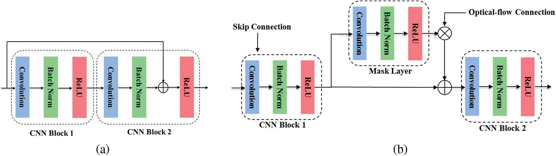
Figure 2: Architecture design for (a) convolutional residual block, and (b) frame optical-flow fusion block

Let x and y be the input and output vector of the CNN Residual block. The output of the 2D convolutional layer is given by

yLj=(∑c=1cLWLj∗xLc+bLj ), j∈[1,cL](2)

Here xLj,yLj, (WLj, bLj), j, and  cL  are the input, output, and model parameters (weight, bias), filter index, number of convolutional filters, respectively of the Lth  layer (depth of CNN layer). For simplicity, we omitted the biases and represent the weight of the convolutional layer as W1, then the output of the convolution layer from Eq. (2) is represented by W1x. The output of CNN block 1 is given, as in (3)

y1=σ(BN(W1x))(3)

Here, BN(⋅), σ(⋅), and y1 are batch normalization operation, non-linear activation layer (ReLU), and output of CNN block 1, respectively. Batch normalization operation is omitted from the equations here onwards for simplifying notations. The output of Convolutional Residual Block is given, as in (4)

y=σ(W2(σ(W1x))+x)(4)

Here, W2 is the weight of the convolutional layer in CNN block 2. The Pooling Block is made of one 2D Convolutional layer with the strides of 2×2 and filter size of 2×2, followed by a Batch Normalization layer, and a ReLU activation layer.

Both prediction branch takes the input of size [b,h,w,c×p], where ‘b’ is the batch size, ‘h’, ‘w’, ‘c’ are height, width, and channel of input image, and ‘p’ is the number of past input sequence. Here, ‘c×p’ represents the input images are stacked before feeding to the network. Let f1:p represents the input sequence of frame encoder module, fP,1:pe represents the output of  eth frame Pooling Block, and f1:pe  represent the output of eth  encoder block (Convolutional Residual Block). Then, the output of frame encoder module (i.e., output of 4th frame encoder block) is given by (6)

fP,1:p4=pool(fR,1:p3)(5)

f1:p4=σ(W4,2f(σ(W4,1ffP,1:p4))+fP,1:p4)(6)

Here f1:p3,(W4,1fW4,2f), and ‘pool’ are the output of 3rd frame encoder block, convolutional weights of Convolutional Residual Block in 4th frame encoder block and pooling operation. Similarly, the output of optical flow encoder module (i.e., output of 4th optical flow encoder block) is given, as in (7)

o1:p4=pool(σ(W4,2o(σ(W4,1ooP,1:p4))+oP,1:p4))(7)

Here (W4,1o,W4,2o) and ‘pool’ are convolutional weights of Convolutional Residual Block in 4th optical-flow encoder block and pooling operation.

3.2.2 Recurrent Network

As seen in Fig. 1, the Recurrent Module consists of two ConvLSTM layers. ConvLSTM is a recurrent layer, just like LSTM, but the internal matrix multiplications are replaced by convolution operations. The ConvLSTM absorbs the properties of Convolution and LSTM and learns both spatial dependencies and temporal relationships between frames. It contains a cell state, a memory, and three gates (input, forget, and output) to protect and control the cell state. The output of the recurrent network is computed by the following operations. At the input gate, the information is added to the cell state in two steps. First, the sigmoid layer decides which input value  (it)  should be updated given, as in (8), then the tanh layer creates a vector of new candidate values (c¯t) given, as in (9). At forget gate, ConvLSTM decides which information  (ft)  should be forgotten from the cell states, as in (10). Based on the update at the input and forget gate, the old cell state ct−1 updates cell state  (ct)  given, as in (11). At the output gate, the ConvLSTM decides which part of the cell state to send to the output  (ot), as in (12). Finally, the output of the recurrent layer is given, as in (13).

it=σ(wxi∗E1:p+whi∗ht−1+wci⊙ct−1+bi)(8)

c¯t=tanh⁡(wxc∗E1:p+whc∗ht−1+bc)(9)

ft=σ(wxf∗E1:p+whf∗ht−1+wcf⊙ct−1+bf)(10)

ct=ft⊙ct−1+it⊙c¯t(11)

ot=σ(wxo∗E1:p+who∗ht−1+wco⊙ct−1+bo)(12)

R1:t=ot⊙tanh⁡(ct)(13)

Here σ(⋅),∗ and ⊙ represent the sigmoid layer, convolution operation and the element-wise multiplication, respectively.

3.2.3 Reconstruction Network

The decoder module in both branches (frame and optical) consists of a series of four decoder blocks followed by an output layer. Each decoder block consists of a 2D transposed convolutional layer, a decoder-convolutional block, and a skip connection from the corresponding encoder block. Except for the decoder-convolutional block, the architecture of the two prediction branches is identical. There is an additional connection layer called the optical-flow connection in the frame-decoder module. On the other hand, the Optical-flow decoder module is similar to the optical-flow convolutional residual block without residual connection. The Transpose Convolutional layer increases the latent representation of the learned spatiotemporal feature map into the original resolution. The Convolution operation grasps the spatial dependencies between pixels before the next upsampling layer. Due to the depth of the neural network, the network suffers not only from the degradation problem but also from the vanishing gradient problem (when the gradient shrinks towards zero during backpropagation, resulting in the weight never updating its value). A skip connection from the feature extraction network to the reconstruction network solves the problem by allowing the gradient to flow directly back from the end layers to the initial layers.

The architecture of the frame decoder-convolutional block (Frame Optical-flow Fusion Block) is shown in Fig. 2b. The output of the transposed convolutional layer is fed into CNN block 1 along with a skip connection (of the appropriate dimension) from the frame encoder module. A mask layer (a 2D convolutional layer with the same number of filters as the previous layer) is generated from the result of CNN block 1. The mask layer is bitwise multiplied with the optical-flow connection of the corresponding dimension from the optical-flow decoder block, then added to the output of CNN block 1 and fed into CNN block 2.

Consider the decoder block are numbered in decreasing order (i.e., the inner-most decoder block number being the highest and the outer-most decoder block numbered as 1). Let o¯1:p e represents the output of  eth optical-flow decoder block. Then, the output of the transpose layer from 1st optical-flow decoder block (o¯T,1:p1) is given, as in (14)

o¯T, 1:p1=transpose(o¯ 1:p2)(14)

Here transpose(⋅) represent 2D transpose convolution with strides of 2×2 and filter kernel size of 2×2. After adding skip connection o1:p1 from frame optical-flow Convolutional Residual Block to the transpose layer of 1th  decoder block, we get the output of transposed layer (o¯TO,1:p1) as in (15), and based on (4), we can compute the output of optical-flow decoder block 1, as in (16)

o¯TO,1:p1=o¯T,1:p1+o1:p1(15)

o¯1:p1=σ(W1,2d(σ(W1,1do¯TO,1:p1)))(16)

Here, σ(⋅) and (W1,1d,W1,2d) represents ReLU activation function and convolutional weights of 1st optical-flow decoder block. For frame decoder, let f¯1:p e represents the output of  eth frame decoder block. Then, the output of transpose layer from 1st frame decoder block (dT,1:p1) is given, as in (17)

f¯T,1:p1=transpose(f¯1:p2)(17)

A skip connection f1:p1 (from frame Convolutional Residual Block) as in (6) along with the output of Transposed Convolutional layer (from 1st frame decoder block) is fed to CNN block 1, the output CNN Block 1 is given as in (19)

f¯T,1:p1=f¯T,1:p1+fR,1:p1(18)

f¯C1,1:p1=σ(W1,1f¯f¯T,1:p1)(19)

Here, σ(⋅) and W1,1f¯ represents ReLU activation function and convolutional weights of CNN block 1 of 1st frame-decoder. At this stage, a mask layer is created to incorporate the future optical motion of the objects. Optical-flow connection from corresponding optical-flow decoder block is multiplied with mask layer and added with the output of CNN block 1 and passed to CNN block 2. The optical flow incorporated with mask layer (f¯M,O,1:p1) is given as in (20) and the output of CNN block 1 (or output of 1st frame-decoder block) as in (21)

f¯M,O,1:p1=σ(WMf¯C1,1:p1)⊙ o¯1:p1(20)

f¯1:p1=σ(W1,2f¯(f¯M,O,1:p1+f¯C1,1:p1))(21)

Here, WM, and W1,2f¯ are the weight of mask convolutional layer and CNN block 2 of 1st frame-decoder block module, and ⊙ represents the bitwise multiplication operation.

Finally, the output of both frame (f^1:p)  and optical-flow (O^1:p) branch is computed by performing convolution operation to output of 1st decoder block from their respective branch with the strides of 1×1, filter kernel size of 3×3 and channel output of 3, followed by batch normalization layer and sigmoid activation function (σ1(⋅)), given as in (22) and (23)

Y^f,1:p=σ1(Woutf¯f¯1:p1)(22)

Y^O,1:p=σ1(WoutO¯o¯1:p1)(23)

Here, Woutf¯ and WoutO¯ are is the convolutional weight of output layer of frame and optical-flow branch, respectively. From Table 1, we have ground truth frame and optical-flow. Hence, we train our model to learn to predict future frame and future optical flow by minimizing the error between the predicted frames and optical-flow from the proposed architecture and ground truth frames and optical-flow from the database.

3.3 Model Training

In this sub-section, we first explain the objective function used for training and then present the pseudo-algorithm for overall model training process.

3.3.1 Loss Function

Since the final output of the model is the images future frames, for learning the parameters in FPNet-OF, we combined the image gradient different loss (GDL), the mean squared difference loss or MSE, and the SSIM loss to measure the quality of the frames between the ground truth images (Yf,1:p) and the predicted image (Y^f,1:p). Similarly, we used the least absolute deviation (L1 loss) to measure the quality of the optical-flow between the ground truth images (YO,1:p) and the predicted image (Y^O,1:p).

Image gradient different loss directly penalizes the differences between neighbor pixels in predicted and ground truth images. The GDL function between the ground truth images (Y) and predicted image (Y^) is given by (24)

ℒGDL(Y,Y^)=∑i,j(||Yi,j−Yi+1,j|−|Y^i,j−Y^i+1,j||+||Yi,j+1−Yi, j|−|Y^i,j+1−Y^i, j||)(24)

where (i,j)  denotes the spatial index of a frame. Similarly, for ground truth image (Y1:p) and predicted image (Y^1:p) which contains the sequence of p frames, the mean gradient difference loss is given by (25)

ℒ¯GDL(Y1:p,Y^1:p)=1h×w∑s=1pℒgdl(Ys,Y^s)(25)

Here, h  and  w represents the height and width of each frame, respectively.

The SSIM evaluates the visual quality differences and similarities between the ground truth image (Y) and the predicted image (Y^) based on luminance, contrast and texture. The SSIM ranges from 0 and 1. SSIM closer to 1 means that the images are nearly identical. Our goal is to minimize the error between the images. Therefore, we subtract the SSIM from one in objective function, i.e., SSIM value closer to 0 is better. The SSIM loss function is calculated as in (26)

ℒSSIM(Y,Y^)1−(2μYμY^+C1)(2σYY^+C2)(μY2+μY^2+C1)(σY2+σY^2+C2)(26)

where μY  and μY^ are the average of Y  and Y^, respectively; σY  and σY^ are the variance of Y  and Y^, respectively; σYY^ is the covariance of Y  and Y^. C1 and C2 are constant and correspond to 0.01 and 0.03, respectively. For the ground truth image (Y1:p) and the predicted image (Y^1:p) which contains the sequence of past p  frames, the SSIM is given as in (27)

ℒSSIM(Y1:p,Y^1:p)=1p∑s=1pℒSSIM(Ys,Y^s)(27)

The mean squared distance loss measure the quality of predicted image by computing a Euclidean distance between the ground truth and predicted image, as in (28)

ℒMSE(Y1:p,Y^1:p)=1w×h∑s=1p(Ys−Y^s)2(28)

The mean least absolute deviation measure the quality of predicted image and is calculated as in (29)

ℒLAD(Y1:p,Y^1:p)=1w×h∑s=1p|Ys−Y^s|(29)

The overall loss function to train frame branch FPNet-OF is given in (30)

ℒ=λ1ℒ¯GDL+λ2(ℒSSIM)+λ3ℒMSE(30)

where λ1, λ2 and λ3 are the weights and are empirically set to 1, 1 and 1 for loss functions mean gradient difference loss, structure similarity measurement loss, and mean square loss, respectively.

The PSNR metric represents the signal-to-noise-ratio based on the mean square error. The PSNR between the ground truth image (Y) and the predicted image (Y^) is given, as in (31). The PSNR value is high if there is less noise between the images.

PSNR(Y,Y^)=10log10⁡maxY^2∑ij(Yi,j−Y^i,j)(31)

where maxY^ is the maximum possible value of the image intensities and (i,j)  denote the spatial index of a frame.

3.3.2 Training Process

Algorithm 1 summarizes the training process of the proposed architecture. The frame and optical-flow dataset (generated using frame dataset, as explained in Section 4.2), the number of the past image sequences p, and the next frame prediction horizon k are the input constraints for training the model, as in Line 1. The weighting factor λ  to balance the objective function and the learning rate  α  is hyper-parameters, as described in line 2. The generation of the input-output sequence of frame and optical-flow datasets for training the model ℱ using the gradient-descent backpropagation and Adam optimization algorithm is shown in lines 4 to 9. We initialized the parameters of the optical-flow prediction branch and the joint optical-flow and frame prediction model as θflow  and  θFPNet−OF, respectively, based on a ‘he uniform’ distribution, as shown in line 10. The training process for the model is shown in lines 11 to 16. The FPNet-OF simultaneously trains the optical-flow prediction model (as shown in lines 12 to 14) and the joint optical-flow and frame prediction model (as shown in lines 12 to 16). Training the optical-flow prediction branch falls under the training process of the FPNet-OF. Therefore, the training of the optical-flow branch is terminated when the termination criteria for the joint model are satisfied. Generally, the termination criteria of the optical-flow prediction model are satisfied earlier compared to the joint model. After the training process is completed, an optimal set of parameters θFPNet−OF  representing the prediction model ℱ is generated as shown line 17.

4  Experiments

In this section, we evaluate the proposed method with multiple real-world data and compare our results with the state-of-the-art frame prediction methods.

4.1 Dataset

In this work, we train and verify the predictive ability of our model on several publicly available datasets, such as Caltech Pedestrian [59], UCF101 [60], CUHK Avenue [61], and ShanghaiTech Campus [62]. To make a fair performance comparison with the existing method, we chose the training and testing dataset the same as mentioned in the original papers.

The Caltech pedestrian data was recorded while driving through regular traffic with the cameras mounted on the vehicle. The dataset consists of about 10 h of video recording with an image resolution of 640 × 480. Since it was recorded in a moving car, the dataset has frequent occlusions and relatively large movements of pixels of vehicles and pedestrians compared to other data sources. The dataset consists of 11 video sets, of which the first six sets are used for training with 71 video sequences, and the last five sets are used for testing with 66 video sequences. The UCF101 dataset comes from YouTube. It contains 101 action categories with 13320 videos at 25 frames per second and of 240 × 320 resolution. UCF101 is commonly used for action prediction and classification. Some of the frequent actions include driving, dancing, push-ups, climbing, crawling, etc. The CUHK Avenue dataset is for abnormal event detection recorded on the CUHK campus. It has 37 video clips (30652 frames), of which 16 video clips (15328 frames) for training and 21 video clips (15324 frames) for testing. The ShanghaiTech campus dataset is for anomaly detection. It contains 13 scenes with complex lighting conditions and camera angles, which include 130 abnormal events. It has 317398 frames for training and 274515 frames for testing.

4.2 Optical Flow Estimation

The optical flow estimation of video frames is calculating the angle and magnitude shift for each pixel. In the statistical approach, the optical-flow is the estimation in two steps: First, the selection of “descriptive” points or visual features (such as corners, edges, ridges, and textures), and then the track “descriptive” in subsequent frames, and calculate the optical change. There are various statistical approaches for estimating optical flow, such as differential techniques [52], region-based matching [63], energy-based methods [64], and phase-based methods [65]. Recent work in this area has addressed approaches based on deep neural network techniques [25,48–53,56] (see Section 2.2 for more details).

In this paper, we have estimated the optical flow based on the work of G. Farneback [66]. Farneback presents a novel algorithm for motion estimation based on two frames, wherein a first step each neighborhood of both frames is approximated by quadratic polynomials, and then the displacement fields are estimated from the polynomial expansions. For simplicity, we used the built-in function ‘calcOpticalFlowFarneback’ by OpenCV in this work. OpenCV also provides other built-in functions for optical flow estimation, such as ‘SparseOpticalFlow’, ‘SparsePyrLKOpticalFlow’, ‘calcOpticalFLowPyrLK’, etc. Algorithm 2 represents the process of optical flow estimation. Two consecutive video frames are the input, as in line 1. The built-in function ‘calcOpticalFlowFarneback’ is algorithm requirement, as in line 2. The input frames should first be converted to a grayscale image, as in line 4. The output of the Farneback algorithm provides two matrices in the Cartesian coordinate system, one for the magnitude shift and the other for the angle, as shown in line 5. The result is converted to a polar coordinate system, as shown in line 6. Finally, we store the magnitude matrix as an image, as in line 7, and discard the angle shift, since we do not use it in the FPNet-OF algorithm.

4.3 Model Parameters and Training Details

The details of the FPNet-OF are explained in this subsection. As shown in Fig. 1, the FPNet-OF consists of 2 identical recurrent convolutional autoencoders branch. Each branch consists of four encoder modules, four decoder modules, a recurrent block, and an input and output layer. Each module contains three hidden layers with a constant number of convolutional filters that perform either down-sampling or up-sampling operations, followed by two convolutional operations. The number of filters is doubled, and the spatial resolution is halved in each subsequent encoder module and vice-versa in the decoder module.

The number of convolutional filters and the spatial resolution are constant in the recurrent block. [32, 64, 128, 256, 512], [512] and [256, 128, 64, 32, 3] are the number of convolutional filters for the hidden layers in the encoder module (input layer and four encoder modules), recurrent block, and decoder module (four decoder modules and output layer), respectively. All convolutional layers, down-sampling, and up-sampling layers have a dropout of 0.1 and batch normalization.

We trained the FPNet-OF for 50 epochs. For the first 10 epochs, we trained both branches of FPNet-OF, and for the remaining 40 epochs, we only trained the frame prediction branch and stopped the training process of the optical-flow prediction branch. On a single GPU, to train the model on the Caltech Pedestrian dataset, the model took 26.5 h for the first 10 epochs, an average of 2.65 h per epoch, and 58.56 h for the remaining 40 epochs, an average of 1.46 h per epoch. The model training time per epoch is decreased by 1.19 h after optical flow learns to predict the accurate future optical flow. To train, we used the Adaptive Moment Estimation (Adam) optimizer for the mini-batch stochastic gradient descent method with momentum parameters, a batch size of 8, and a learning rate of 1e-4. We implemented the FPNet-OF using the Tensorflow deep learning library on an Ubuntu 18.04.4 machine with 1 NVIDIA TITAN Xp Graphics Card with a GPU memory of 11 GB.

4.4 Result and Analysis

For quantitative evaluation, we use three metrics video prediction: structural similarity, mean square error, and PSNR as given in Eqs. (26), (28), and (31), respectively. A metric value close to zero is better for MSE, close to one is better for SSIM, and a higher positive value is better for PSNR. In this work, we set the length of the past input sequence to two images (i.e., two frames and two optical-flow) for predicting the next frame and take a long input history to forecast multiple time steps in the future. Some of the works, such as PredNet [8], Retro-Cycle GAN [31], BeyondMSE [38], Dual Motion GAN [54], and DMMNet [55] uses more than two input images to predict the next frame. We evaluate FPNet-OF as follows: First, we analyze an ablation study on various components to design our proposed architecture. Then, we compare next-frame prediction predictions with other state-of-the-art approaches for various datasets. Finally, we compare the multiple time-step forecasting ability of FPNet-OF with other state-of-the-art approaches.

4.4.1 Ablation Study

We carried out an ablation study under various settings by excluding different parts from our proposed architecture one by one to see the impact of each designed module. Table 2 compares the quantitative result with various architectural designs. The red ‘cross’ in the table indicates that the proposed architecture is designed without that corresponding part(s) whereas, the green ‘tick’ represents that the architecture contains that particular part(s). The simple convolutional autoencoder architecture with skip connections performs adequately for the next frame prediction. It is evident from Ablation studies 2 and 3. The network performance is boosted with the addition of a recurrent block, as seen in Ablation 4. From ablation studies 4 & 6, we can say the addition of recurrent components has a higher impact on the model performance than that of the optical-flow connections. But, with the addition of optical flow connections, recurrent blocks, and skip connections, the performance of the model is improved significantly, as seen in Ablation 8. Therefore, the use of all the components for predicting the future frame is crucial. Fig. 3 shows some typical qualitative comparisons of the ablation studies 3, 6, and 8 with the ground truth. Since all three ablation studies have high performance, the difference in the prediction is very subtle.

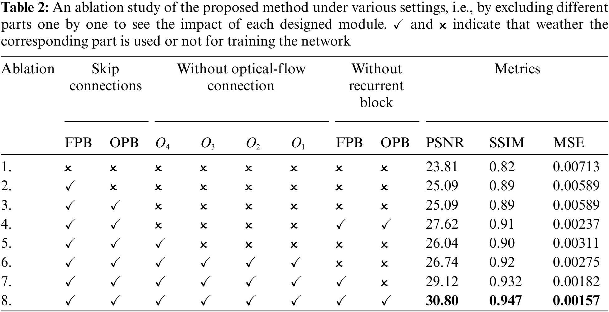
Figure 3: Qualitative comparisons of the ablation studies with the ground truth for one-frame prediction result on some calTech pedestrian dataset

4.4.2 Next Frame Prediction Performance

Caltech Pedestrian Dataset: At first, we generate frame and optical-flow triples for training and testing, where each triplet consists of three consecutive images, the first two as input and last as predicting ground truth. Next, we resized the frames and optical flow to 256 × 256 and finally normalized their pixels value in the range of 0 and 1. Table 3 shows the qualitative evaluation of our approach compared to several state-of-the-art methods such as PredNet [8], Retro-Cycle GAN [31], BeyondMSE [38], ContextVP [47], Dual Motion GAN [54], and DMMNet [55] for next-frame prediction on Caltech Pedestrian Dataset. The results for the other model are from original papers or cited papers. From Table 3, we can see that in terms of MSE and PSNR, our model achieves the highest performance compared to the other, and in terms of SSIM, our model achieves the highest performance compared to all except DMMNet. Our model achieves an SSIM value of 0.947, 0.3 percent lower than DMMNet, while the MSE and PSNR performance is significantly high. Our model achieves the MSE value of 0.00157, which is around half compared to the DMMNet MSE value of 0.00317 while maintaining nearly equal SSIM. Fig. 4 shows the qualitative comparisons of FPNet-OF with other state-of-art approaches on the next frame prediction. It shows the comparison between Ground Truth, Proposed (Ours), Retro-Cycle GAN [31], and ContextVP [47] from left to right, respectively.

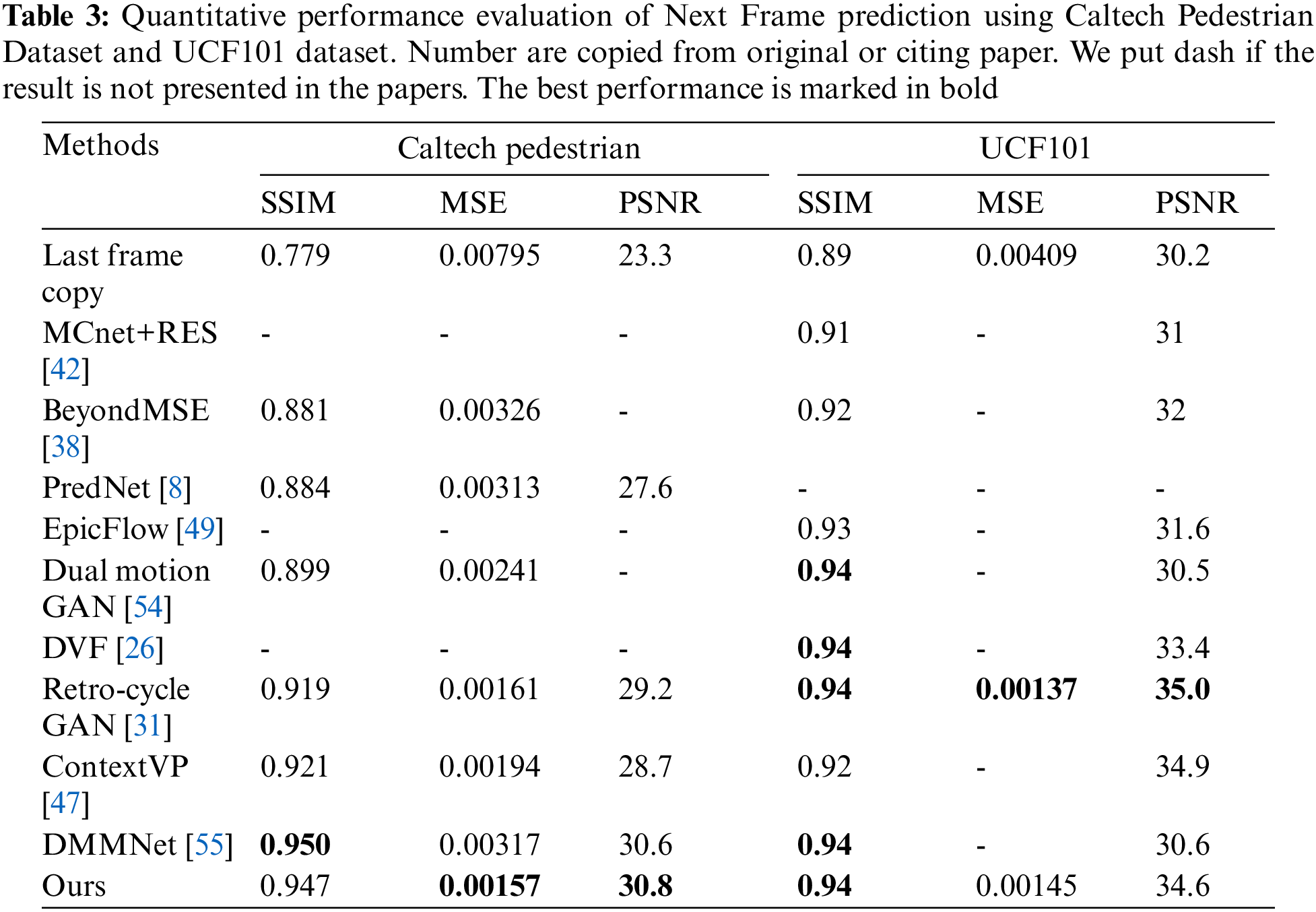
Figure 4: Qualitative comparisons of the next-frame prediction by ours, Retro-Cycle GAN [31], and Contextvp [47] on Caltech pedestrian dataset

From Fig. 4, we can see that the prediction result of the FPNet-OF is smoother compared to other methods because our model learns both the optical motion of the objects and spatial-temporal dependencies between the images to predict the future frame. Fig. 5 shows some typical comparisons of the next frame prediction results of the FPNet-OF with the ground truth, under various conditions, such as an object moving across, the scene with a large number of dynamic bodies, under different lighting, at an intersection, and image with occlusion, etc. In all the cases, our model shows superior performance.

Figure 5: Some typical qualitative comparisons of our method with ground truth for next-frame prediction under various conditions, such as vehicle moving across, the scene with a large number of dynamic bodies, under different lighting, at an intersection, and image with occlusion on Caltech pedestrian dataset

UCF 101 Dataset: Similar to the Caltech dataset, we first generate frame and optical-flow triples for training and testing, resize them to the resolution of 256 × 256, and normalized their pixels value in the range of 0 and 1. Table 3 shows the qualitative evaluation of our approach compared to several state-of-the-art methods such as DVF [26], Retro-Cycle GAN [31], BeyondMSE [38], MCnet + RES [42], ContextVP [47], EpicFlow [49], Dual Motion GAN [54], and DMMNet [55] for next-frame prediction. The results for the other model are from original papers or cited papers. From Table 3, we can see that the prediction performance of our model is equal to other high-performing models like [26,31,54], and [55] in terms of SSIM. On the other hand, our model performance is slightly lower in MSE and PSNR to Retro-cycle GAN (the highest value). Fig. 4 shows the qualitative comparison of the FPNet-OF with other state-of-the-art approaches. It shows the comparison between ground truth, ours (proposed), Retro-Cycle GAN [31], ContextVP [47] from left to right, respectively. The figure shows that our model shows consistent performance compared to other top performing models.

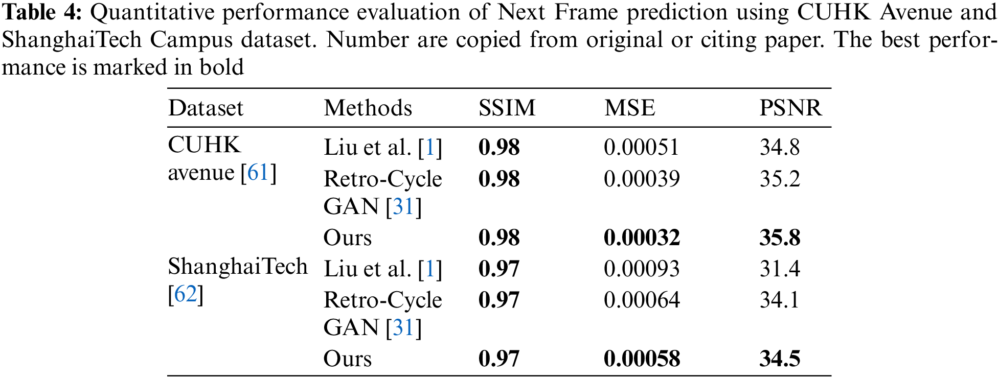
For surveillance datasets, such as CUHK Avenue and ShanghaiTech: Similar to the Caltech pedestrian dataset and the UCF101 dataset, we first generate frame and optical-flow triples for training and testing, resize them to the resolution of 256 × 256, and normalized their pixels value in the range of 0 and 1. Table 4 shows the qualitative evaluation of our approach compared to two other state-of-the-art methods: Liu et al. [1] and Retro-Cycle GAN [31] for next-frame prediction. The results for the other model are from original papers or cited papers. From Table 4, we can say that FPNet-OF outperforms other models in MSE and PSNR for both surveillance datasets and have an equal SSIM value compared to high-performing state-of-the-art approaches.

4.4.3 Multiple Frame Prediction Performance

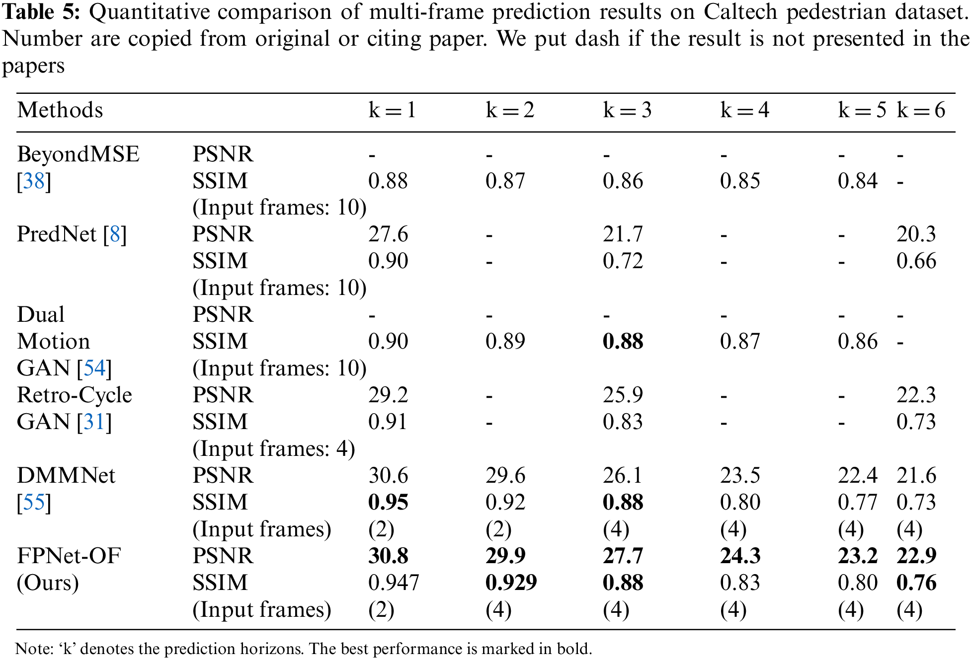
The quantitative comparison of multi-frame prediction on the Caltech pedestrian dataset is evaluated in this subsection. We compared the prediction performance of FPNet-OF with other state-of-the-art frame prediction models, such as PredNet [8], Retro-Cycle GAN [31], BeyondMSE [38], Dual Motion GAN [54], and DMMNet [55]. We evaluate the prediction performance in terms of SSIM and PSNR up to six-frame in the future.

For multi-step prediction, we first generate frame and optical-flow input-output image batch. Each batch contains ten images, the first four for input and the last six for ground truth. Then each image is resized to the resolution of 256 × 256, and pixels are normalized in the range of 0 and 1. First, we predict the next frame and then concatenate the result to the input sequence to create a new input sequence to forecast the next frame. This procedure is repeated until the desired prediction horizon is not achieved. Table 5 shows the quantitative comparison of multi-frame prediction results. For a prediction horizon equal to 1, the SSIM value of DMMNet [55] has the highest value of 0.95, which is 0.03 higher than our proposed model (FPNet-OF), which achieves the second position, and the rest of the study have much lower values averaging around 0.9. In terms of the PSNR value, our model achieves 30.8, which is the highest among all the other studies. For the prediction horizon equal to 2, FPNet-OF attains the highest performance in terms of the SSIM and PSNR 0.929 and 29.9, respectively. The DMMNet [55] scheme comes second compared to our model. For k equals 3, in terms of SSIM, FPNet-OF attains 0.88, which is equal to DMMNet [55] and Dual Motion GAN [54], whereas, in terms of PSNR, our model outperforms other schemes. For k equals 4 & 5, our models perform better than DMMNet [55] in both SSIM & PSNR. But Dual Motion GAN [54] to achieve the values in terms of SSIM. For prediction horizons equal to 6, FPNet-OF attains 0.79 and 22.9 in terms of SSIM and PSNR, respectively, which are the highest value in contrast to PredNet [8], Retro-Cycle GAN [31], and DMMNet [55]. The SSIM and PSNR value decreases as we go further in time. The FPNet-OF predicts frames with the higher SSIM for second, third, and sixth future frames and higher PSNR for all six future frames. From Table 5, we can see the SSIM value of FPNet-OF and DMMNet [55] outperforms all other schemes by a large margin for the next frame prediction due to adaptive fusing of optical-flow estimation to frame prediction. But, for large prediction horizons, the SSIM performance of Dual Motion GAN [54] is better than FPNet-OF and DMMNet [55] because of adversarial learning. From Table 5, we can also see that the state-of-the-art frame prediction schemes are good at predicting multi-frame only up to a few prediction horizons. After a certain threshold, the performance of the networks decreases drastically and is not suitable for frame prediction. Therefore, in this experiment, we limit the prediction horizon to 6.

5  Conclusions

In this work, we proposed an end-to-end deep neural network architecture, FPNet-OF (Frame Prediction Network with multiple-branch inputs (optical flow and original frame)), to predict the future video frame. The FPNet-OF consists of two branches named frame prediction branch and optical-flow prediction branch. Frame prediction branch exploits spatiotemporal information from past frame input sequence to predict the next frame. The optical-flow prediction branch learns the spatiotemporal relations of object motion from the input past optical-flow image to generate the future optical-flow image. Due to the adaptively fusing of future object-motion with the future frame generator, the hybrid model generates superior future frame prediction compared to other state-of-the-art.

As discussed in Sub-Section 4.1.1, we conclude the optimal architecture of the FPNet-OF should consist of skip connection in both branches, optical-flow connection at every decoder block to provide excellent performance. From the result analysis Sub-Sections 4.4.2–4.4.3, we can see that FPNet-OF achieves superior performance in frame prediction on multiple datasets. In future work, incorporating recent ideas like adversarial training or explicit background modeling with our model can improve prediction performance. Furthermore, we can investigate for large-step video prediction like a few seconds in the future rather than a few frames, which is more desirable for real-world applications.

Acknowledgement: This work was supported by Incheon National University Research Grant in 2017.

Funding Statement: The authors received no specific funding for this study.

Conflicts of Interest: The authors declare that they have no conflicts of interest to report regarding the present study.

References

1. W. Liu, W. Luo, D. Lian and S. Gao, “Future frame prediction for anomaly detection-A new baseline,” 2018 in IEEE/CVF Conf. on Computer Vision and Pattern Recognition (CVPR), Salt Lake City, UT, USA, pp. 6536–6545, 2018. [Google Scholar]

2. M. Chaabane, A. Trabelsi, N. Blanchard and R. Beveridge, “Looking ahead: Anticipating pedestrians crossing with future frames prediction,” in 2020 IEEE Winter Conf. on Applications of Computer Vision (WACV), Snowmass Village, CO, USA, pp. 2286–2295, 2020. [Google Scholar]

3. N. Deo and M. M. Trivedi, “Multi-modal trajectory prediction of surrounding vehicles with maneuver based LSTMs,” in Proc. IEEE Intelligent Vehicles Symp. (IV), Changshu, Suzhou, China, pp. 1179–1184, 2018. [Google Scholar]

4. J. -R. Xue, J. -W. Fang and P. Zhang, “A survey of scene understanding by event reasoning in autonomous driving,” International Journal of Automation and Computing, vol. 15, no. 3, pp. 249–266, 2018. [Google Scholar]

5. P. Kumar, M. Perrollaz, S. Lefevre and C. Laugier, “Learning-based approach for online lane change intention prediction,” in 2013 IEEE Intelligent Vehicles Symp. (IV), Gold Coast, QLD, Australia, pp. 797–802, 2013. [Google Scholar]

6. H. Saleem, F. Riaz, A. Shaikh, K. Rajab, A. Rajab et al., “Optimizing steering angle predictive convolutional neural network for autonomous car,” Computers, Materials & Continua, vol. 71, no. 2, pp. 2285–2302, 2022. [Google Scholar]

7. W. Park and M. Kim, “Deep predictive video compression using mode-selective uni-and bi-directional predictions based on multi-frame hypothesis,” IEEE Access, vol. 9, pp. 72–85, 2021. [Google Scholar]

8. W. Lotter, G. Kreiman and D. Cox, “Deep predictive coding networks for video prediction and unsupervised learning,” in 5th Int. Conf. on Learning Representations (ICLR), Toulon France, 2017. [Google Scholar]

9. J. -J. Leou, Y. -L. Chang and J. -S. Wu, “Robot operation monitoring for collision avoidance by image sequence analysis,” Pattern Recognition, vol. 25, no. 8, pp. 855–867, 1992. [Google Scholar]

10. D. Pedro, J. P. Matos-Carvalho, J. M. Fonseca and A. Mora, “Collision avoidance on unmanned aerial vehicles using neural network pipelines and flow clustering techniques,” Remote Sensing, vol. 13, no. 13, pp. 2643, 2021. [Google Scholar]

11. D. Deotale, M. Verma, P. Suresh, S. K. Jangir, M. Kaur et al., “HARTIV: Human activity recognition using temporal information in videos,” Computers, Materials & Continua, vol. 70, no. 2, pp. 3919–3938, 2022. [Google Scholar]

12. K. Zeng, W. B. Shen, D. Huang, M. Sun and J. C. Niebles, “Visual forecasting by imitating dynamics in natural sequences,” in Int. Conf. on Computer Vision (ICCV), Venice, Italy, pp. 3018–3027, 2017. [Google Scholar]

13. P. Thamizhazhagan, M. Sujatha, S. Umadevi, K. Priyadarshini, V. S. Parvathy et al., “AI based traffic flow prediction model for connected and autonomous electric vehicles,” Computers, Materials & Continua, vol. 70, no. 2, pp. 3333–3347, 2022. [Google Scholar]

14. N. Ranjan, S. Bhandari, H. P. Zhao, H. Kim and P. Khan, “City-wide traffic congestion prediction based on CNN, LSTM and transpose CNN,” IEEE Access, vol. 8, pp. 81606–81620, 2020. [Google Scholar]

15. N. Ranjan, S. Bhandari, P. Khan, Y. -S. Hong and H. Kim, “Large-scale road network congestion pattern analysis and prediction using deep convolutional autoencoder,” Sustainability, vol. 13, no. 9, pp. 5108, 2021. [Google Scholar]

16. C. Bregler, “Learning and recognizing human dynamics in video sequences,” in Proc. of IEEE Computer Society Conf. on Computer Vision and Pattern Recognition, San Juan, PR, USA, pp. 568–574, 1997. [Google Scholar]

17. M. Brand, N. Oliver and A. Pentland, “Coupled hidden markov models for complex action recognition,” in Proc. of IEEE Computer Society Conf. on Computer Vision and Pattern Recognition, San Juan, PR, USA, pp. 994–999, 1997. [Google Scholar]

18. A. M. Lehrmann, P. V. Gehler and S. Nowozin, “Efficient nonlinear markov models for human motion,” in Proc. of the IEEE Conf. on Computer Vision and Pattern Recognition (CVPR), Columbus, OH, USA, pp. 1314–1321, 2014. [Google Scholar]

19. V. Mahadevan, W. Li, V. Bhalodia and N. Vasconcelos, “Anomaly detection in crowded scenes,” in 2010 IEEE Computer Society Conf. on Computer Vision and Pattern Recognition, San Francisco, CA, USA, pp. 1975–1981, 2010. [Google Scholar]

20. Y. W. Teh and G. E. Hinton, “Rate-coded restricted boltzmann machines for face recognition,” Advances in Neural Information Processing Systems (NIPS), Denver, CO, USA, pp. 908–914, 2001. [Google Scholar]

21. D. Neupane and J. Seok, “Bearing fault detection and diagnosis using case western reserve university dataset with deep learning approaches: A review,” IEEE Access, vol. 8, pp. 93155–93178, 2020. [Google Scholar]

22. D. Neupane and J. Seok, “A review on deep learning-based approaches for automatic sonar target recognition,” Electronics, vol. 9, no. 11, pp. 1972, 2020. [Google Scholar]

23. S. Bhandari, N. Ranjan, P. Khan, H. Kim and Y. -S. Hong, “Deep learning-based content caching in the fog access points,” Electronics, vol. 10, no. 4, pp. 512, 2021. [Google Scholar]

24. S. Bhandari, H. Kim, N. Ranjan, H. P. Zhao and P. Khan, “Optimal cache resource based on deep neural network for fog radio access networks,” Journal of Internet Technology, vol. 21, no. 4, pp. 967–975, 2020. [Google Scholar]

25. J. Walker, C. Doersch, A. Gupta and M. Hebert, “An uncertain future: Forecasting from static images using variational autoencoders,” in Proc. of the European Conf. on Computer Vision (ECCV), Amsterdam, The Netherlands, pp. 835–851, 2016. [Google Scholar]

26. Z. Liu, R. A. Yeh, X. Tang, Y. Liu and A. Agarwala, “Video frame synthesis using deep voxel flow,” in Proc. IEEE Int. Conf. on Computer Vision (ICCV), Venice, Italy, pp. 4473–4481, 2017. [Google Scholar]

27. K. Gregor, I. Danihelka, A. Graves, D. J. Rezende and D. Wierstra, “DRAW: A recurrent neural network for image generation,” in Proc. of the 32nd Int. Conf. on Machine Learning, Lille, France, pp. 1462–1471, 2015. [Google Scholar]

28. N. Srivastava, E. Mansimov and R. Salakhudinov, “Unsupervised learning of video representations using LSTMs,” in Proc. Int. Machine Learning Society (ICML), Lille, France, pp. 843–852, 2015. [Google Scholar]

29. Q. Ke, M. Bennamoun, H. Rahmani, S. An, F. Sohel et al., “Learning latent global network for skeleton-based action prediction,” IEEE Transactions on Image Processing, vol. 29, pp. 959–970, 2020. [Google Scholar]

30. D. Wang, Y. Yuan and Q. Wang, “Early action prediction with generative adversarial networks,” IEEE Access, vol. 7, pp. 35795–35804, 2019. [Google Scholar]

31. Y. Kwon and M. Park, “Predicting future frames using retrospective cycle GAN,” in 2019 IEEE/CVF Conf. on Computer Vision and Pattern Recognition (CVPR), Long Beach, CA, USA, pp. 1811–1820, 2019. [Google Scholar]

32. V. Badrinarayanan, A. Kendall and R. Cipolla, “SegNet: A deep convolutional encoder-decoder architecture for image segmentation,” IEEE Transactions on Pattern Analysis and Machine Intelligence, vol. 39, no. 12, pp. 2481–2495, 2017. [Google Scholar] [PubMed]

33. X. Liu, Z. Deng and Y. Yang, “Recent progress in semantic image segmentation,” Artificial Intelligence Review, vol. 52, no. 2, pp. 1089–1106, 2019. [Google Scholar]

34. N. Elsayed, A. S. Maida and M. Bayoumi, “Reduced-gate convolutional LSTM architecture for next-frame video prediction using predictive coding,” in 2019 Int. Joint Conf. on Neural Networks (IJCNN), Budapest, Hungary, pp. 1–9, 2019. [Google Scholar]

35. W. Yu, Y. Lu, S. M. Easterbrook and S. Fidler, “Efficient and information-preserving future frame prediction and beyond,” in Proc. of the Int. Conf. on Learning Representations (ICLR), Addis Ababa, Ethiopia, 2020. [Google Scholar]

36. R. Haziq and B. Fernando, “A Log-likelihood regularized KL divergence for video prediction with a 3D convolutional variational recurrent network,” in 2021 IEEE Winter Conf. on Applications of Computer Vision Workshops (WACVW), Waikola, HI, USA, pp. 209–217, 2021. [Google Scholar]

37. Y. Lu, K. Mahesh Kumar, S. S. Nabavi and Y. Wang, “Future frame prediction using convolutional VRNN for anomaly detection,” in 2019 16th IEEE Int. Conf. on Advanced Video and Signal Based Surveillance (AVSS), Taipei, Taiwan, pp. 1–8, 2019. [Google Scholar]

38. M. Mathieu, C. Couprie and Y. LeCun, “Deep multi-scale video prediction beyond mean square error,” in 4th Int. Conf. on Learning Representations (ICLR), San Juan, Puerto Rico, 2016. [Google Scholar]

39. J. Oh, X. Guo, H. Lee, R. L. Lewis and S. Singh, “Action-conditional video prediction using deep networks in atari games,” Advances in Neural Information Processing Systems, Montreal, Quebec, Canada, pp. 2863–2871, 2015. [Google Scholar]

40. M. Ranzato, A. Szlam, J. Bruna, M. Mathieu, R. Collobert et al., “Video (language) modeling: A baseline for generative models of natural videos,” CoRR, vol. abs/1412.6604v5, 2016. [Google Scholar]

41. C. Vondrick, H. Pirsiavash and A. Torralba, “Generating videos with scene dynamics,” Advances in Neural Information Processing Systems, Barcelona, Spain, pp. 613–621, 2016. [Google Scholar]

42. R. Villegas, J. Yang, S. Hong, X. Lin and H. Lee, “Decomposing motion and content for natural video sequence prediction,” in Proc. ICLR, Toulon, France, pp. 1–22, 2017. [Google Scholar]

43. T. Xue, J. Wu, K. Bouman and B. Freeman, “Visual dynamics: Probabilistic future frame synthesis via cross convolutional networks,” in Proc. Advances in Neural Information Processing Systems (NIPS), Barcelona, Spain, pp. 91–99, 2016. [Google Scholar]

44. D. Tran, L. Bourdev, R. Fergus, L. Torresani and M. Paluri, “Learning spatiotemporal features with 3D convolutional networks,” in Int. Conf. on Computer Vision(ICCV), Santiago, Chile, pp. 4489–4497, 2015. [Google Scholar]

45. C. Finn, I. Goodfellow and S. Levine, “Unsupervised learning for physical interaction through video prediction,” Advances in Neural Information Processing Systems (NIPS), Barcelona, Spain, pp. 64–72, 2016. [Google Scholar]

46. W. Lotter, G. Kreiman and D. Cox, “Unsupervised learning of visual structure using predictive generative networks,” in Int. Conf. on Learning Representation (ICLR), San Juan, Puerto Rico, 2016. [Google Scholar]

47. W. Byeon, Q. Wang, R. K. Srivastava and P. Koumoutsakos, “ContextVP: Fully context-aware video prediction,” in Proc. of the European Conf. on Computer Vision (ECCV), Munich, Germany, pp. 781–797, 2018. [Google Scholar]

48. C. Liu, J. Yuen and A. Torralba, “Sift flow: Dense correspondence across scenes and its applications,” IEEE Transactions on Pattern Analysis and Machine Intelligence, vol. 33, no. 5, pp. 978–994, 2011. [Google Scholar] [PubMed]

49. J. Revaud, P. Weinzaepfel, Z. Harchaoui and C. Schmid, “EpicFlow: Edge-preserving interpolation of correspondences for optical flow,” in Proc. IEEE Conf. on Computer Vision and Pattern Recognition (CVPR), Boston, MA, USA, pp. 1164–1172, 2015. [Google Scholar]

50. D. Mahajan, F. -C. Huang, W. Matusik, R. Ramamoorthi and P. Belhumeur, “Moving gradients: A path-based method for plausible image interpolation,” in SIGGRAPH09: Special Intrest Group on Computer Graphics and Interactive Techniques Conf., New Orleans, LA, Article 42, pp. 1–11, 2009. [Google Scholar]

51. Z. Luo, B. Peng, D. Huang, A. Alahi and L. Fei-Fei, “Unsupervised learning of long-term motion dynamics for videos,” in Conf. on Computer Vision and Pattern Recognition (CVPR), Honolulu, HI, USA, pp. 7101–7110, 2017. [Google Scholar]

52. B. K. P. Horn and B. G. Schunck, “Determining optical flow,” Artificial Intelligence, vol. 17, pp. 185–203, 1981. [Google Scholar]

53. A. Dosovitskiy, P. Fischer, E. Ilg, P. Häusser, C. Hazirbas et al., “FlowNet: Learning optical flow with convolutional networks,” in IEEE Int. Conf. on Computer Vision (ICCV), Santiago, Chili, pp. 2758–2766, 2015. [Google Scholar]

54. X. Liang, L. Lee, W. Dai and E. P. Xing, “Dual motion GAN for futureflow embedded video prediction,” in Proc. IEEE Int. Conf. on Computer Vision (ICCV), Venice, Italy, pp. 1762–1770, 2017. [Google Scholar]

55. S. Li, J. Fang, H. Xu and J. Xue, “Video frame prediction by deep multi-branch mask network,” IEEE Transactions on Circuits and Systems for Video Technology, vol. 31, no. 4, pp. 1283–1295, 2021. [Google Scholar]

56. N. Sedaghat, “Next-flow: Hybrid multi-tasking with next-frame prediction to boost optical-flow estimation in the wild,” CoRR, vol. abs/1612.03777v2, 2017. [Google Scholar]

57. K. He, X. Zhang, S. Ren and J. Sun, “Deep residual learning for image recognition,” in 2016 IEEE Conf. on Computer Vision and Pattern Recognition (CVPR), Las Vegas, NV, USA, pp. 770–778, 2016. [Google Scholar]

58. B. Li and Y. He, “An improved ResNet based on the adjustable shortcut connections,” IEEE Access, vol. 6, pp. 18967–18974, 2018. [Google Scholar]

59. P. Dollár, C. Wojek, B. Schiele and P. Perona, “Pedestrian detection: An evaluation of the state of the art,” Transactions on Pattern Analysis and Machine Intelligence (TPAMI), vol. 34, no. 4, pp. 743–761, 2012. [Google Scholar]

60. K. Soomro, A. R. Zamir and M. Shah, “UCF101: A dataset of 101 human action classes from videos in the wild,” CRCV-TR-1 2–01, 2012. [Google Scholar]

61. M. Ravanbakhsh, M. Nabi, E. Sangineto, L. Marcenaro, C. Regazzoni et al., “Abnormal event detection in videos using generative adversarial nets,” in Int. Conf. on Image Processing (ICIP), Beijing, China, pp. 1577–1581, 2017. [Google Scholar]

62. W. Luo, W. Liu and S. Gao, “A revisit of sparse coding based anomaly detection in stacked RNN framework,” in Int. Conf. on Computer Vision (ICCV), Venice, Italy, pp. 341–349, 2017. [Google Scholar]

63. J. Barron, D. Fleet and S. Beauchemin, “Performance of optical flow techniques,” International Journal of Computer Vision, vol. 12, pp. 43–47, 1994. [Google Scholar]

64. D. J. Heeger, “Optical flow using spatiotemporal filters,” International Journal of Computer Vision, vol. 1, pp. 279–302, 1988. [Google Scholar]

65. B. Buxton and H. Buxton, “Computation of optical flow from the motion of edge features in image sequences,” Image and Vision Computing, vol. 2, no. 2, pp. 59–74, 1984. [Google Scholar]

66. G. Farneback, “Two-frame motion estimation based on polynomial expansion,” Scandinavian Conf. on Image Analysis (SCIA), Halmstad, Sweden, pp. 363–370, 2003. [Google Scholar]