MLD-MPC Approach for Three-Tank Hybrid Benchmark Problem

1  Introduction

Recently, many researchers have been interested in the field of HDSs because such systems have continuously been implemented in areas like industrial process control, robotics, and chemical processes. Indeed, apart from their continuous dynamics such as pressure, flow, or current, many processes contain discrete components like valves or switches. Since HDSs involve the interaction of continuous and discrete dynamics, their modeling is extremely difficult. Hybrid modeling of systems is intended for different problem-solving tasks, namely control law synthesis [1,2], stability [3,4], modeling and analysis [5,6].

Note that several approaches to modeling hybrid systems have already been mentioned in the literature. Some of these combine Algebraic Differential Equations (ADEs) with Discrete-Event Simulation (DES) models in a single structure. The hybrid automaton [7] is one of the most used modeling formalisms joined to this class of mixed approaches. Hybrid Automata (HA) have mainly been adopted for the analysis and verification of hybrid systems [8–10]. However, this modeling framework cannot be tailored in the case of control hybrid system synthesis. Another class of approaches is based on the transformation of propositional logic expressions into linear inequalities of binary variables. The author in [11] has introduced MLD formalism, one of the most widely used models for the analysis and control synthesis designed for hybrid systems [12–14]. MLD formalism has the benefit of gathering all continuous dynamics, logic rules, and system constraints under a single representation to synthesize the conventional hybrid control methods. In this framework, approaches like MPC control may be used to design hybrid control laws.

The MPC is an advanced optimization control technique that has widely been applied both in the research control community and in various process industry sectors. In the case of hybrid systems, many researchers were keen to adopt this control approach, such as [15,16]. As a result, the MPC has emerged as a systematic controller synthesis that is very promising for handling on/off inputs, logic states, switching linear dynamics, and logic constraints of the system. The MPC principle aims at solving an optimization problem on a finite prediction horizon. Given the hybrid nature of the systems, the associated optimization problem is of the MIP type that must be solved with the appropriate techniques. Several authors proved that B&B is one of the most effective techniques for MIP and thus it is often the most adopted [17–20].

The purpose of the present study is to apply the level control of a Three-Tank Hybrid System (TTHS). TTHS has been considered in numerous research works as a typical benchmark study of HDSs [21–24]. The level control problem of the TTHS is crucial to the HDS study. Various approaches have been recently utilized in this framework of the study. Reference [21] illustrated a linear quadratic controller-based closed-loop control of a TTHS. In [23], an estimation-based control scheme for nonlinear autonomous TTHS is discussed. Moreover, [24] conducted an adaptive PI controller for a TTHS. In the present work, the considered TTHS has 128 operating modes. To build a model imitating the real studied system, all these operating modes must be considered. In other words, one must consider the continuous and discrete dynamics of the system during the modeling process. On the other hand, to control this class of large-scale hybrid systems, it is necessary to use advanced control techniques. The proposed approach is MPC control based on the MLD model, which constitutes a compelling control framework. The most obvious benefit of this control framework is to exploit the benefits of MPC’s predictive and constraint management functions with MLD’s ability to model HDSs.

This paper is divided as follows; the second section provides an overview of HDSs. In the third section, the MLD approach is described along with the following steps to obtain the MLD model. Then, the formulation of the MPC strategy for MLD systems is detailed in section four. In section five, the MLD model of the TTHS is carried out first, then the hybrid MPC control is applied to the system, and the associated results are further discussed. Finally, in the last section, the conclusion is elaborated.

2  Hybrid Dynamical System

A real dynamic process is often a complex system that exhibits both continuous and discrete dynamic behavior. It is then evident that this kind of system cannot be represented satisfyingly with a purely continuous or purely event-driven dynamic. The notion of HDS designates a dynamic system formed by the coupling and interaction of continuous and discrete systems (Fig. 1) [25].

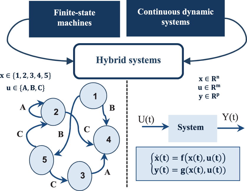
Figure 1: Continuous dynamics interacting with discrete events [25]

Generally, an HDS may be seen as the aggregation of a Discrete-Event System (DES), Continuous-Dynamic System (CDS), and interfaces that manage the interactions between the two evolutions (continuous and discrete).

The diagram in Fig. 2 [25] represents the generic structure of an HDS. The discrete part of the HDS is associated with a DES. The models representing discrete-event systems are finite state automata, Petri nets, and State Charts. The continuous part is represented by a set of continuous models, which is often based on ordinary differential equations. In contrast, the Continuous/Discrete (C/D) and Discrete/Continuous (D/C) interfaces reflect the interaction between the two parts. The interaction phenomenon between these types of dynamics is called a hybrid phenomenon.

Figure 2: Generic structure of an HDS [25]

3  Description of the MLD Formalism

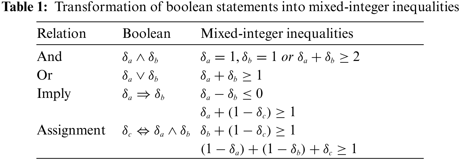
MLD systems appear as an appropriate framework for modeling several classes of hybrid systems and solving control problems. MLD system is a linear system bound by inequalities, including real and binary variables. The MLD formalism is founded on transforming propositional logical statements into mixed inequalities. The conceptual details of this transformation are well enlightened in [11]. Relations of this type occur at the interfaces (Fig. 2), and their transformation into inequality allows us to formulate and include them in a global mathematical model. Using a set of fundamental transformations, the Boolean variables characterizing the discrete part in Fig. 2 could be converted into binary linear inequalities. Some equivalences are reported in Table 1.

At the C/D interface, binary auxiliary variables δ are introduced to make it possible to describe the influence of the continuous state on the discrete dynamics (events) by mixed inequalities Eq. (1) [11].

[f(x)≤0]⇔[δ=1](1)

The above assignment expression can be converted to [25]:

{g(x)≤H(1−δ)g(x)≥ε+(h−ε)δ(2)

where H is the upper bound of g and h its lower bound, while ε is a small positive number.

Likewise, at the D/C interface (Fig. 2), the introduction of the real auxiliary variables z allows for considering mode changes and the influence of the discrete state on the continuous dynamics (e.g., open valve). The following equation defines the equality relation [11]:

z=δg(x)(3)

Then, this equation is transformed into mixed inequalities [25]:

{z≥hδz≤Hδz≤g(x)−h(1−δ)z≥g(x)−H(1−δ)(4)

The real auxiliary variables z are in the equations of continuous dynamics, and the binary auxiliary variables δ are in the equations of discrete dynamics. The foundations of MLD formalism are laid.

The generic structure of the MLD system is highlighted in Fig. 3 [25].

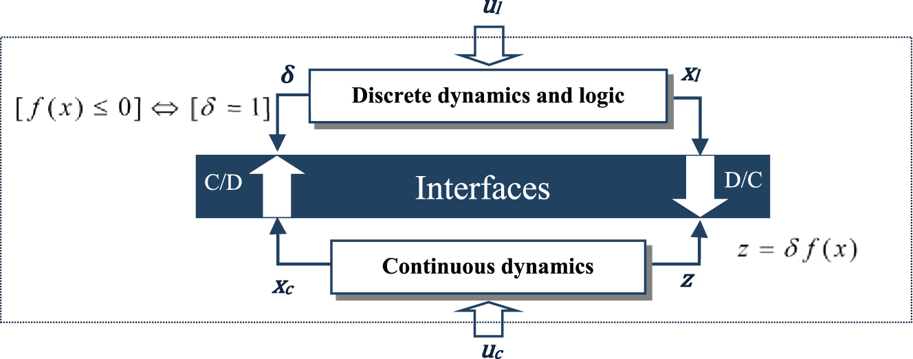
Figure 3: Generic structure of the MLD system [25]

Considering, on the one hand, the continuous linear dynamics of the system and, on the other hand, the transformations of logical relations into inequalities. The general form of the discrete-time MLD system is as follows [25]:

xk+1=Axk+B1uk+B2δk+B3zk(5a)

yk=Cxk+D1uk+D2δk+D3zk(5b)

E2δk+E3zk≤E4xk+E1uk+E5(5c)

with the state:

x=(xcxl)withxc∈ℜnxc,  xl∈{0, 1}nxl, nx≜nxc+nxl(6)

the input:

u=(ucul)withuc∈ℜnuc,  ul∈{0, 1}nul, nu≜nuc+nul(7)

and the output:

y=(ycyl)withyc∈ℜnyc,  yl∈{0, 1}nyl, ny≜nyc+nyl(8)

δ∈{0,1}rl are auxiliary binary variables, z∈ℜnyc representing continuous auxiliary variables that appear in the transformations. A, B1,…, B3, C, D1 ,…, D3, E1,…, E5 are matrices of the system of equations with appropriate dimensions. Assuming, x(k) is the current state and u(k) is the input, the time-evolution of Eq. (5) is determined by finding feasible values for δ(k) and z(k) satisfying Eq. (5c) and then by computing x(k+1) and y(k) from Eqs. (5a)–(5b). One way of proceeding is to consider a linear mixed optimization problem to examine the pair’s existence (δ(k),z(k)).

4  MPC of MLD Systems

MPC is one of the internal model control techniques for predicting the system’s output over a future prediction horizon. This method is based on the adoption of a receding horizon strategy. It calculates an optimal control sequence that minimizes the cost function for a constrained dynamical system. The first element of the computed control sequence is applied to the system. In the following time step, a new sequence is calculated to replace the previous one. MPC strategy is presented in Fig. 4 [26].

Figure 4: Model predictive control strategy [26]

Several works presented in the literature have adopted the MPC control for MLD systems such as [27–29]. In this case, the optimal control problem that must be solved is a Mixed Optimization Problem (MOP). It can be solved with some of the MIP techniques, either Mixed Integer Quadratic Programming (MIQP) or Mixed Integer Linear Programming (MILP). Recent works were discussed, presenting MILP and MIQP techniques in hybrid MPC design [30–32].

4.1 Problem Position

Once the MLD model of the system has been well-posed, the optimization problem related to the MPC approach can be written as a MOP.

Let the current time be k and k+N as the final time, xk is the current state, (xc,uc) a reference trajectory value, and find U=(u0T,u1T,…,uN−1T)T the sequence of commands in the prediction horizon which moves the state from xk to xc.

At each sampling step, the problem to be solved can be established as [11]:

minUJN(x0,U)=minU∑k=0(N−1)(||xk+1−xc||Qx2+||yk−yc||Qy2+||uk−uc||Qu2+||δk−δc||Qδ2+||zk−zc||Qz2)(9)

subject to (for k=0 to N−1):

xk+1=Axk+B1uk+B2δk+B3zk(10a)

yk=Cxk+D1uk+D2δk+D3zk(10b)

E2δk+E3zk≤E4xk+E1uk+E5(10c)

xN=xc(10d)

The pair (δc,zc) is determined from the pair (xc,uc) called the equilibrium pair, by solving the MILP problem in a way similar to the feasibility test. yc is the output setpoint, and N is the length of the prediction horizon.

The weighting matrices have the following properties: Qx,u are definite symmetric positive, and Qδ,z,y are definite symmetric semi-positive. Within an online MPC, the stability of the controlled system is guaranteed by the choice of the terminal state constraint under feasibility assumptions.

The optimization problem involves the control variables u and the auxiliary variables δ and z. Thereby, the vector to be optimized is augmented: from the control perspective, the optimal control U is being researched, but from the optimization perspective, (UTΔTZT)T are being sought, where Δ and Z are the sequences of variables δ and z on the horizon.

Problem Eq. (9) can be written in the following quadratic form [11]:

minV=12VTHV+fTV(11)

subject to:

AinV≤bin(12)

AeqV=beq(13)

where V=(UTΔTZT)T with U=[uk,…,uk+N−1]T,Δ=[δk,…,δk+N−1]T,Z=[zk,…,zk+N−1]T.

Fig. 5 shows the design of the MPC control strategy based on the MLD model. The optimal solution V∗ to the predictive control problem (11) is chosen as the system control signal u(t). At each iteration, due to the integer variables δ and z used in the MLD model, the control problem should be solved using a MIP algorithm.

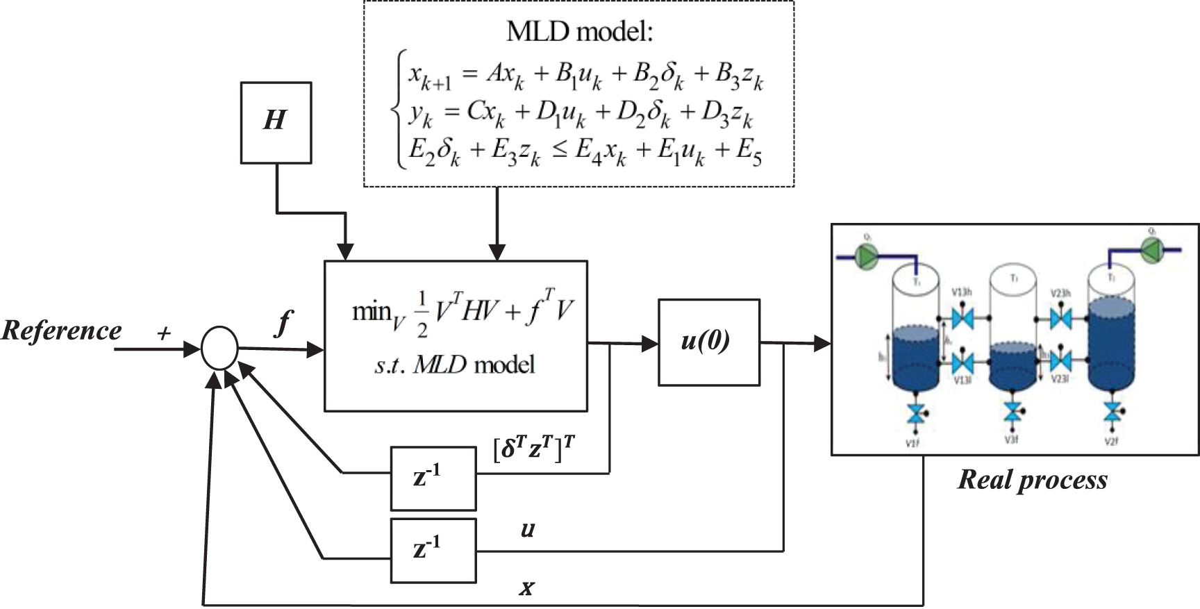
Figure 5: Strategy of the MLD-MPC control for a hybrid system

4.2 Mixed Integer Programming

The minimization problem Eq. (9) can be solved with MIQP based on an exhaustive enumeration technique, that is, generating all possible solutions to find the optimal one.

The number of binary optimization variables is:

Nl=N(nul+rl)(14)

The maximum number of solved Qp problems is:

NmaxQp=2Nl(15)

Since the optimization time grows exponentially with the problem size, MIQPs problems are classified as NP-complete. To avoid exhaustive enumeration of integer variables of the problem and therefore reduce the number of solutions to be tested, several methods have been approved such as the B&B method.

B&B is the commonly used technique for solving MIQP, which aims to eliminate the branches associated with a partial solution deemed unfeasible using lower and upper bounds.

The B&B method is based on alternating a separation step and an evaluation step. The first step consists in dividing a problem into disjoint sub-problems, resulting in a binary search tree. The evaluation of each tree node will indicate whether the latter can contain an optimal solution. As described in Fig. 6, the problem associated with each node is solved. If the problem is infeasible, that tree branch is marked, and there is no need to further explore it. Then, the node is expanded to include a new binary variable. The optimal solution V∗ is chosen among the feasible solutions with the lowest cost concerning the objective function.

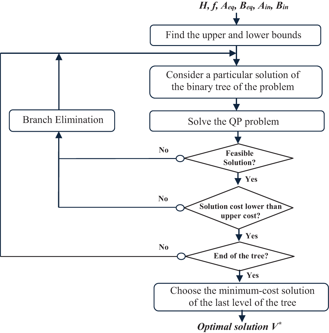
Figure 6: Branch-and-bound algorithm

5  Application: Three-Tank Hybrid System

5.1 Description of the Three-Tank Hybrid System

In the present simulation study, a three-tank process is considered for implementing the proposed MLD-MPC approach. The studied system is composed of three tanks interconnected with valves, as shown in Fig. 7 [25]. Tank T1 and tank T2 are supplied with water by two pumps with flow rates Q1 and Q2 ranging between 0 and Qmax=2.10−4 m3/s. The liquid levels in the tanks are the variables to be controlled denoted h1, h2 and h3 with a maximal height hmax=1 m. The upper control valves (V13h,V23h), positioned at a height hv=0.8 m, and the lower control valves (V13l,V23l) can only take two states: fully opened or fully closed. The valves V1f, V2f and V3f define outgoing flows of tanks equal to 0.1 m3/s.

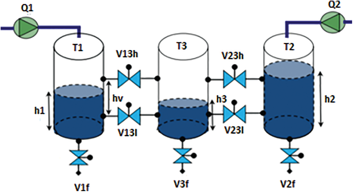
Figure 7: Three-tank benchmark process [25]

5.2 Modeling of the Three-Tank Process in MLD Framework

The equations of levels in tanks are derived from the conservation law of the mass as follows [25]:

h˙1=1Sc(Q1−Q13l−Q13h−Q1f)(16a)

h˙2=1Sc(Q2−Q23l−Q23h−Q2f)(16d)

h˙3=1Sc(Q13l+Q13h+Q23l+Q23h−Q3f)(16c)

where Sc is the cross-sectional area of each tank and Q denotes the liquid flow. Torricelli’s law provides the relations of the flows through the valves with a linearized form of the system as follows:

Q13l≈kV13l(h1−h3)(17a)

Q23l≈kV23l(h2−h3)(17b)

Qif≈kVifhifori∈{1, 2, 3}(17c)

where k=aSv2g/hmax, a is an associated constant to the liquid, Sv represents the section of valves and g is the acceleration due to gravity.

For the flow  Q13h, it is necessary to consider the configuration of the different cases for liquid levels h1 and h3:

Ifh1≥hv and h3≥hvthenQ13h=khV13h(h1−h3)(18a)

Ifh1≤hv and h3≥hv thenQ13h=khV13h(hv−h3)(18b)

Ifh1≥hv and h3≤hvthen Q13h=khV13h(h1−hv)(18c)

Ifh1≤hv and h3≤hv thenQ13h=0(18d)

where kh=aSv2g/(hmax−hv).

Equally, it is possible to determine the flow Q23h.

Let us consider, on the one hand, the state space of the TTHS, which is partitioned into eight regions, and on the other hand, the possible constraints of the states of the valves (0/1) are considered. The studied system then has 128 operating modes.

By introducing the following variables, it is possible to obtain the MLD model of the studied TTHS: x=y=[h1 h2 h3]T, u=[Q1 Q2 V13l V23l V13h V23h]T, δ=[δ1 δ2 δ3]T and Z=[z1 z2 z3 z13l z23l z13h z23h]T.

where:

[δi=1]⇔[hi≥hv] fori=1, 2, 3(19a)

zi=δi(hi −hv) fori=1, 2, 3(19b)

zi3l=Vi3l(hi −h3) fori=1, 2(19c)

zi3h=Vi3h(zi −z3) fori=1, 2(19d)

Finally, the tool HYSDEL (HYbrid Systems Description Language) [33] generates a computational MLD model. It is a high-level modeling language for hybrid systems in discrete time.

5.3 MLD-MPC of TTHS

A first simulation concerning the evolution of the open-loop system using the MLD model is realized. The system is simulated for 500 s, and the following initial conditions are: h10=0.1 m, h20=0.9 m and h30=0.1 m. The manipulated variables in this study case are: U=[10−4;10−4;1;1;0;0].

Fig. 8 presents the responses of levels in the three-tank system within the MLD model. According to this open-loop response, it is obvious that the evolution of levels is far from the desired references. Then the open-loop system using the MLD model is unstable.

Figure 8: Dynamical evolution of TTHS in open loop (MLD model): (a) h1(t), (b) h2(t), (c) h3(t)

The objective of the MLD-MPC control strategy is to reach the liquid levels h1=0.6 m, h2=0.8 m and h3=0.5 m. Using a sample time T=10 s, simulations of 30×T=300 s have been achieved for the horizon prediction N=2.

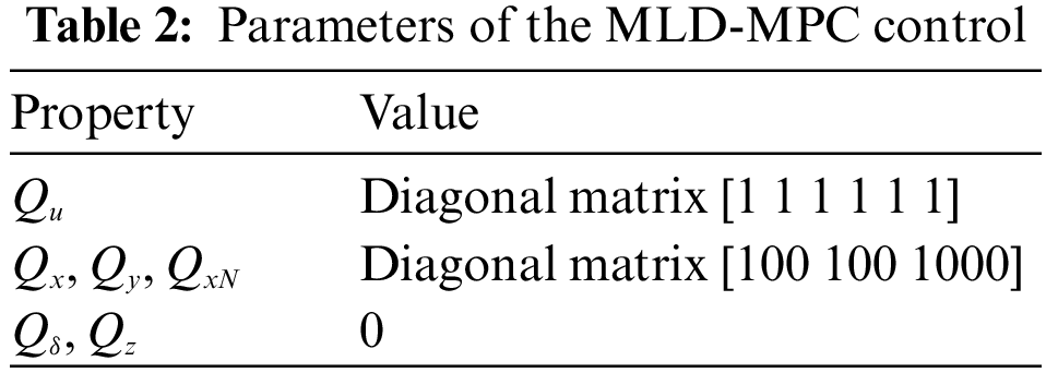
The simulations of the system are achieved using a CPLEX solver with the B&B algorithm [34]. For best results in terms of output precision, the weight matrices should be adjusted. The choice is initially to enhance the output variable weighting matrix’s value relative to the other variables. Consider a fast switching of the control signal, which is undesirable for the system, after several simulation tests the appropriate weighting values have been determined. The weighting matrix values for the MLD-MPC control are listed in Table 2.

By applying the MLD-MPC control, the simulation results of the closed-loop system are illustrated in Fig. 9 for the liquid levels and Fig. 10 for continuous and discrete control signals. From Fig. 9, it is apparent that the system converges to desired level specifications. The tracking errors for the tanks are highlighted in Table 4, for T1 and T2 are close to zero and for tank T3 less than 1%. Note that the level h3(t) gives away oscillations around the desired level h3=0.5 m as it does not correspond to an equilibrium point level. These oscillations do not disturb the main object of the control. They are induced by the opening and closing of the interaction valve V13l presented in Fig. 10 to ensure adjustment of the level h3(t) to its desired reference.

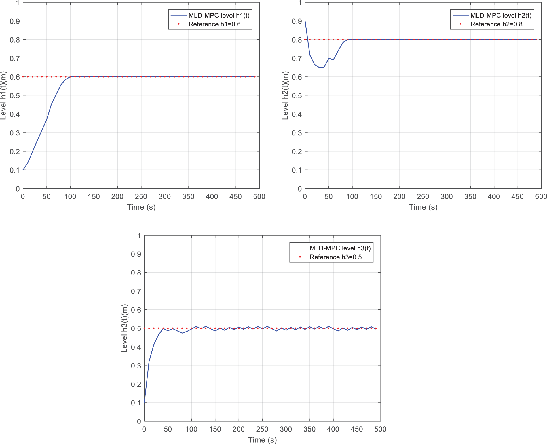
Figure 9: Dynamical evolution of TTHS in closed-loop (MLD-MPC): (a) h1(t), (b) h2(t), (c) h3(t)

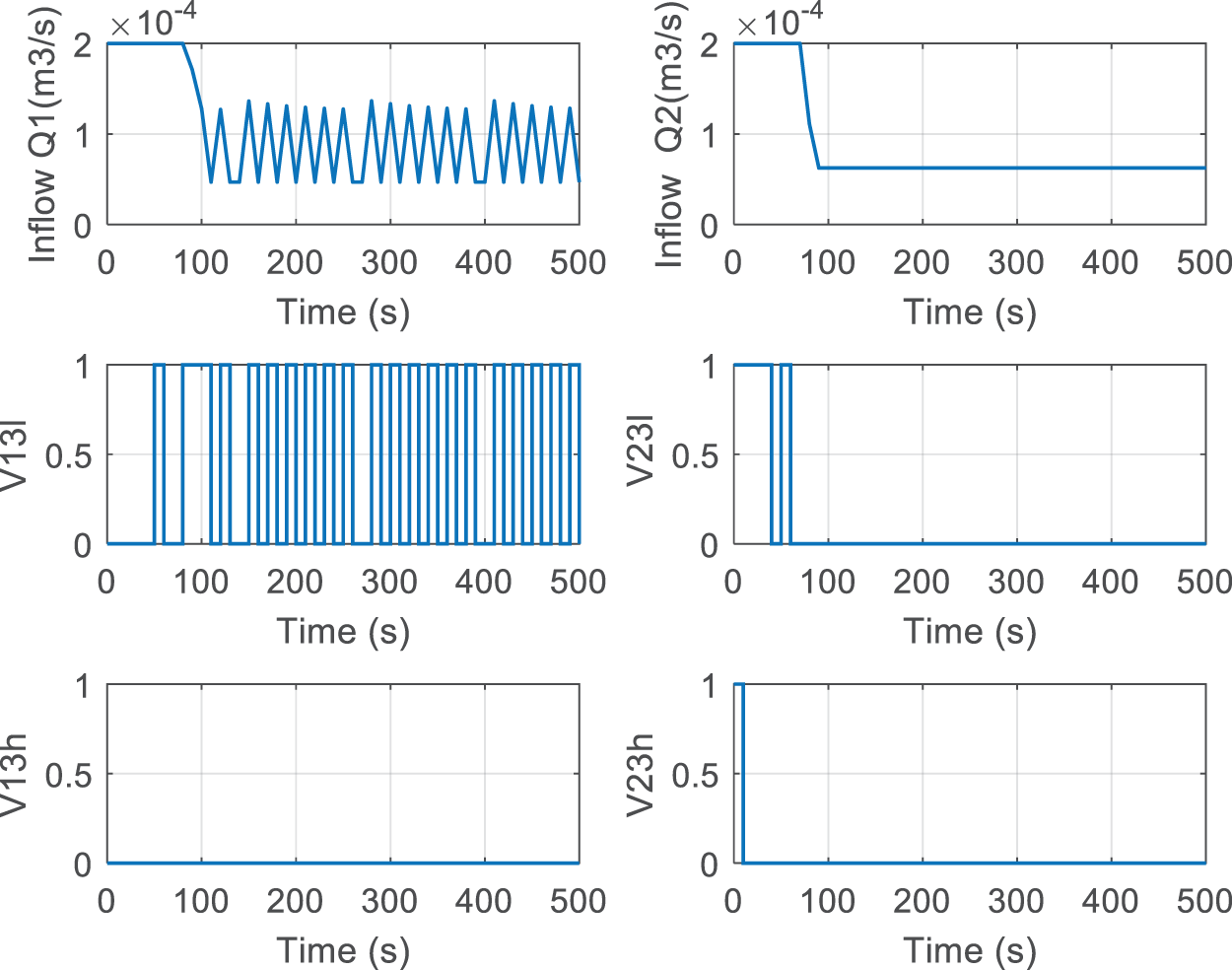
Figure 10: Control signals with MLD-MPC (u=[Q1 Q2 V13l V23l V13h V23h ]T)

Fig. 9 shows the evolutions of the levels h1(t) and h3(t) that do not present oscillations. The level h1(t) is manipulated by the inflow Q1 and the valve V13l. The valve V13h is permanently closed and does not allow the liquid exchange between the two tanks T1 and T3. In contrast, the level h2(t) is manipulated by the inflow Q2 and the two valves [V23l V23h]. After reaching the setpoint h2=0.8 m, the two valves kept closed and the inflow Q2 became constant at 6.24.10−5 m^{3}/s.

Another simulation was performed concerning the robustness of the MLD-MPC control against disturbances while keeping the same previous parameters illustrated in Table 2. Disturbances are considered as liquid leaks from the valve V1f of tank T1 equal to 0.05m^{3}/s (50% compared with the nominal value of the outgoing flow from V1f).

The evolutions of the levels are illustrated in Fig. 11. The level h1(t) oscillates around the desired setpoint that is no longer a point of equilibrium in the presence of disturbances. Fig. 12 presents the manipulated inputs adjusted by the MLD-MPC controller. The disturbances rejection is assumed by acting on the inflow Q1, and the state of the valve V13l that induced the oscillations.

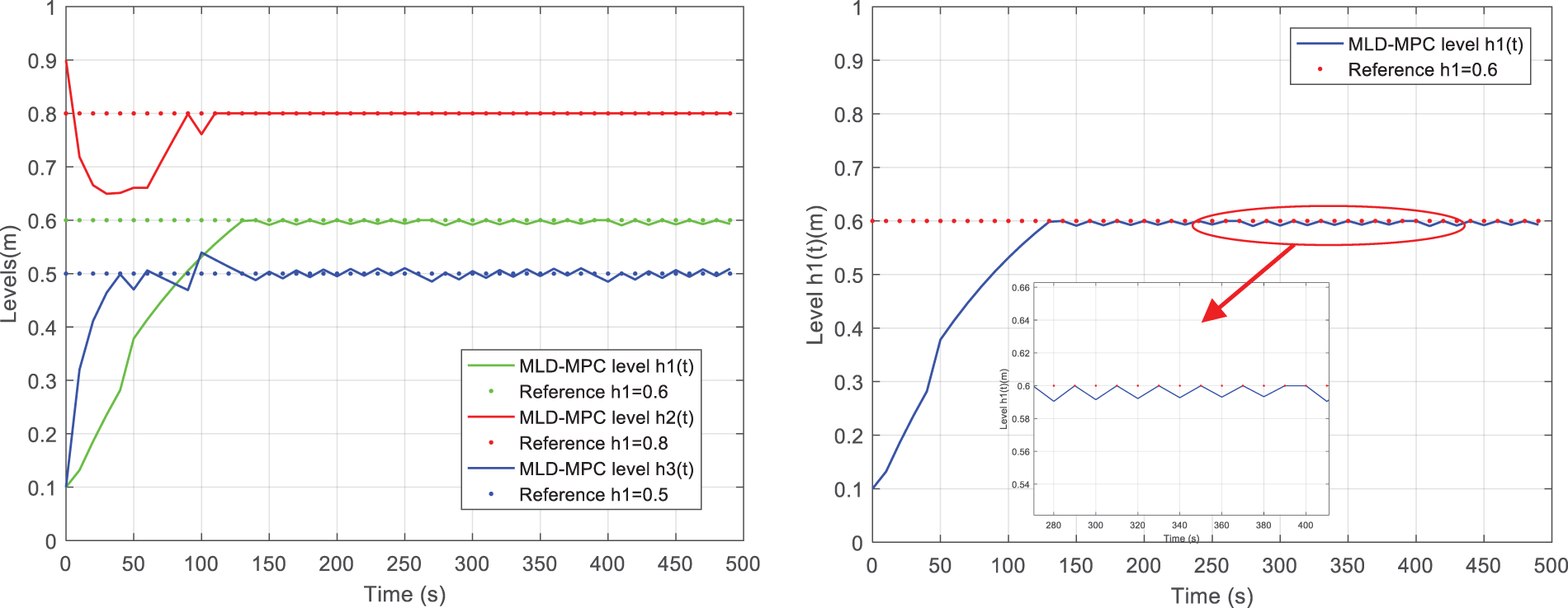
Figure 11: Dynamical evolution of TTHS in closed-loop (MLD-MPC) in the presence of disturbances: (a) h1(t), h2(t) and h3(t), (b) h1(t)

Figure 12: Control signals in the presence of disturbances (u=[Q1 Q2 V13l V23l V13h V23h ]T)

The evidence from this study is that the MLD-MPC control made the system converge to desired equilibrium points even if it is affected by disturbances. Also, the steady-state error for the level is deficient with the value of 6.8.10−9%.

To demonstrate the effectiveness of MLD-MPC control such as accuracy and high robustness in the case of hybrid systems, the proposed method is compared to a standard MPC approach under different conditions (nominal conditions and in the presence of disturbances). The standard MPC, based on quadratic optimization, is synthesized with the constrained linear system model.

The used linear model is gained by linearizing the nonlinear system around a single operating mode corresponding to: (h1 < hv ), (h2 < hv ), (h3  < hv ), (V13l=1), (V23l=1),(V13h=0), (V23h=0).

Additionally, the matrices (A, B, C, and D) that represent the system state space are as shown:

A=[−0.0273 00.0248 0 −0.02730.0248 0.0248 0.0248−0.0521],B=[31.847100 031.84710],C=[100 010 001], D=[000 000](20)

To provide a comparison between the controllers, the exact values of the weighting matrices are applied. Table 3 details the parameter of the standard MPC.

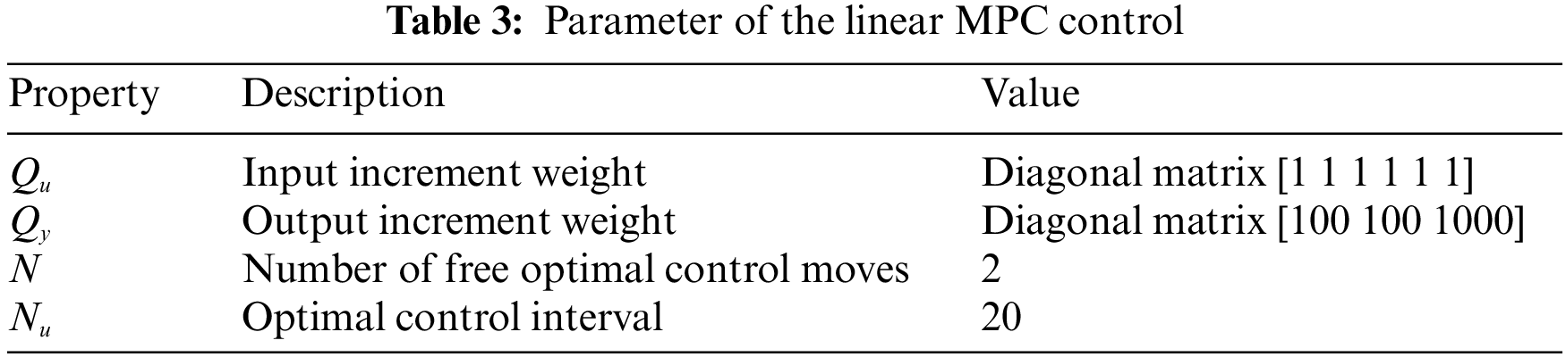
Fig. 13 plots the evolution of tank levels using standard MPC (dash-dotted lines) and MLD-MPC approach. The two continuous manipulated inputs generated by standard MPC are pinpointed in Fig. 14. With the standard MPC based on a single linear model, it is highlighted in Fig. 13 that the system does not follow the desired trajectory. In addition, from Table 4, it is evident that the values for tracking errors are significant in both cases (normal conditions and in the presence of disturbances).

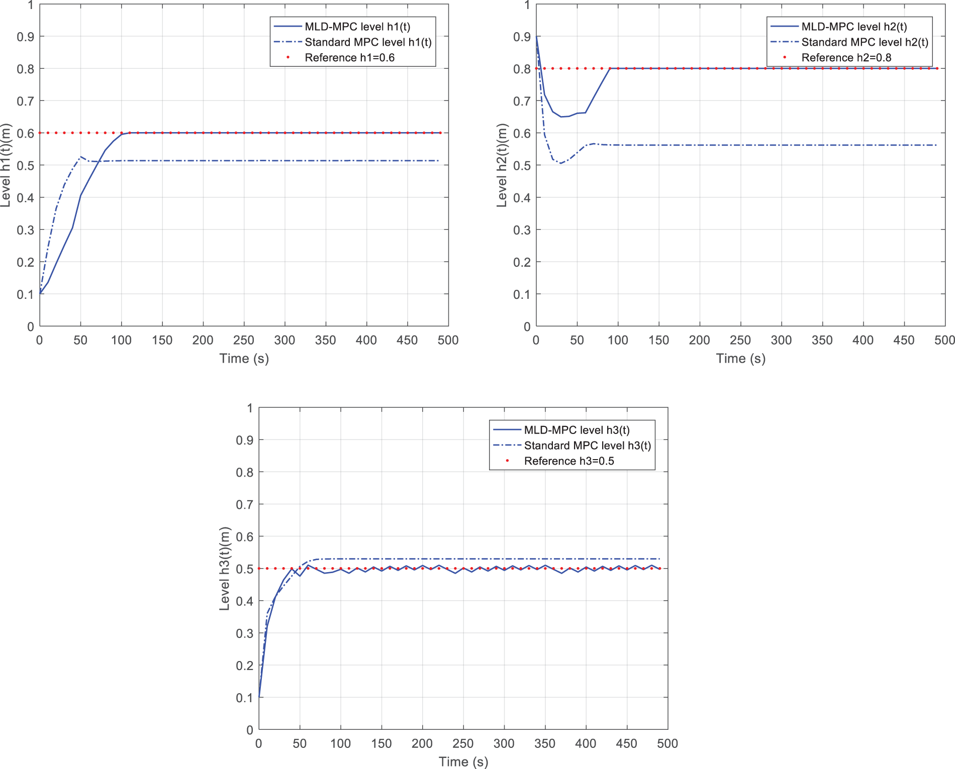
Figure 13: Dynamical evolution of TTHS (MLD-MPC/standard MPC): (a) h1(t), (b) h2(t), (c) h3(t)

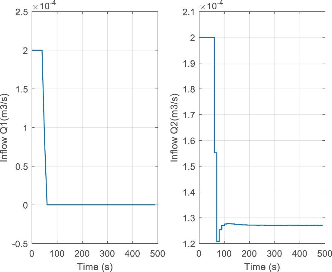
Figure 14: Control signals (standard MPC): u=[Q1 Q2]T

As established from Table 4, the MLD-MPC controller for the TTHS has respectable performance, and the steady-state error is very low (less than 0.1% in nominal conditions and less than 0.6% in the presence of disturbances). Whereas using standard MPC control, the system outputs didn’t converge to the desired setpoint, and the tracking errors are notable whether under normal conditions (more significant than 18.76% for h2(t)) or in the presence of disturbances (more significant than 20.98% for h1(t)). These results prove that the standard MPC is not suitable for the control of the TTHS.

As expected, the linear model doesn’t provide a good approximation of the TTHS. Indeed, the studied system operates in 128 modes, whereas the linear model approximates the system around a single operating point. This hurts the performance of the system; the desired performance is guaranteed locally only when the system operates around this linearization point [25]. The MLD modeling approach relies on approximating the nonlinear system by multiple linearizations for various operating points; the system can switch from one operating mode to another. This modeling framework is essential for synthesizing hybrid system controllers to preserve the most incredible performance under diverse operating modes.

In general, it is impossible to model or control HDSs with sufficient precision, neither by continuous systems theory approaches nor by discrete systems theory approaches. In this respect, the consideration of the discrete input variables of the system is essential to guarantee the desired performances for the closed-loop system.

6  Conclusion

In this paper, an MPC strategy of a three-tank system has been proposed using an MLD model. The MLD formalism was used to obtain a robust hybrid system modeling framework to synthesize the MPC control for the TTHS. Then, the proposed MLD-MPC control based on MIQP has been developed with the B&B algorithm. Various simulations have been exhibited, and the results demonstrate the strengths of the proposed hybrid approach, such as precision and efficiency in normal conditions and high robustness in the presence of disturbances. Subsequently, this paper introduced a comparative study between the MLD-MPC control and the standard MPC based on a single linear constrained model. The results reveal the superior performances of the hybrid MLD-MPC approach compared to the standard MPC. The strengths of the hybrid approach lie both in the behavior approximation level and in the consideration of discrete variables. Research into solving this problem of predictive control of HDSs is already underway. It is highly recommended to introduce more advanced optimization methods. Similarly, there has been a growing interest in using heuristic methods instead of the B&B algorithm. Our study will also be applied to a real process to experimentally validate this approach.

Funding Statement: The authors received no specific funding for this study.

Conflicts of Interest: The authors declare that they have no conflicts of interest to report regarding the present study.

References

1. B. Altin, P. Ojaghi and R. G. Sanfelice, “A model predictive control framework for hybrid dynamical systems,” IFAC-PapersOnLine, vol. 51, no. 20, pp. 128–133, 2018. [Google Scholar]

2. M. Robba and M. Rossi, “Optimal control of hybrid systems and renewable energies,” Energies, vol. 15, no. 1, pp. 78, 2021. [Google Scholar]

3. A. A. Martynyuk, “Elements of the theory of stability of hybrid systems,” International Applied Mechanics, vol. 51, no. 3, pp. 243–302, 2015. [Google Scholar]

4. A. R. Teel and J. P. Hespanha, “Stochastic hybrid systems: A modeling and stability theory tutorial,” in 2015 54th IEEE Conf. on Decision and Control (CDC), Osaka, Japan, pp. 3116–3136, 2015. [Google Scholar]

5. D. Vošček, A. Jadlovská and D. Grigl’ák, “Modelling, analysis and control design of hybrid dynamical systems,” Journal of Electrical Engineering, vol. 70, no. 3, pp. 176–186, 2019. [Google Scholar]

6. K. Kumar, T. Aggrawal, V. Verma, S. Singh, S. Singh et al., “Modeling and simulation of hybrid system,” International Journal of Advanced Science and Technology, vol. 29, no. 4s, pp. 2857–2867, 2020. [Google Scholar]

7. N. Lynch, R. Segala and F. Vaandrager, “Hybrid i/o automata,” Information and Computation, vol. 185, no. 1, pp. 105–157, 2003. [Google Scholar]

8. Y. -J. Ning, H. -P. Ren and J. Li, “An improved switching controller for boost converter based on hybrid automata model,” in 2019 Chinese Automation Congress (CAC), Hangzhou, China, pp. 4598–4602, 2019. [Google Scholar]

9. V. V. Skobelev and V. G. Skobelev, “Some problems of analysis of hybrid automata,” Cybernetics and Systems Analysis, vol. 54, no. 4, pp. 517–526, 2018. [Google Scholar]

10. Z. Xiao, K. Chen, B. He, Z. Wu and Y. Zhang, “A type of hybrid automata model using in laboratory optimal management,” in 2020 IEEE 4th Information Technology, Networking, Electronic and Automation Control Conf. (ITNEC), Chongqing, China, vol. 1, pp. 2065–2069, 2020. [Google Scholar]

11. F. Borrelli, A. Bemporad and M. Morari, Predictive Control for Linear and Hybrid Systems, Cambridge University Press, 2017. [Online]. Available: https://www.cambridge.org [Google Scholar]

12. Y. Zhang, X. Chu, Y. Liu and Y. Liu, “A modelling and control approach for a type of mixed logical dynamical system using in chilled water system of refrigeration system,” Mathematical Problems in Engineering, vol. 2019, pp. 1–12, 2019. [Google Scholar]

13. C. Liang, X. Xu and F. Wang, “MLD based model and validation of DM-PHEV in mode transition process,” in 2021 40th Chinese Control Conf. (CCC), Shanghai, China, pp. 1405–1412, 2021. [Google Scholar]

14. T. Zanma, S. Akiba, K. Hoshikawa and K. Z. Liu, “Cruise control for a two-wheeled mobile vehicle using its mixed logical dynamical system model,” IEEE Transactions on Industrial Informatics, vol. 16, no. 5, pp. 3145–3156, 2019. [Google Scholar]

15. J. Ng and H. H. Asada, “Model predictive control and transfer learning of hybrid systems using lifting linearization applied to cable suspension systems,” IEEE Robotics and Automation Letters, vol. 7, no. 2, pp. 682–689, 2021. [Google Scholar]

16. P. PS, S. Bhartiya and R. D. Gudi, “Modeling and predictive control of an integrated reformer–membrane–fuel cell–battery hybrid dynamic system,” Industrial & Engineering Chemistry Research, vol. 58, no. 26, pp. 11392–11406, 2019. [Google Scholar]

17. B. Legat, R. M. Jungers and J. Bouchat, “Abstraction-based branch and bound approach to Q-learning for hybrid optimal control,” Learning for Dynamics and Control, vol. 144, pp. 263–274, 2021. [Google Scholar]

18. P. Hespanhol, R. Quirynen and S. Di Cairano, “A structure exploiting branch-and-bound algorithm for mixed-integer model predictive control,” in 2019 18th European Control Conf. (ECC), Naples, Italy, pp. 2763–2768, 2019. [Google Scholar]

19. N. Adelgren and A. Gupte, “Branch-and-bound for biobjective mixed integer programming,” INFORMS Journal on Computing, vol. 34, no. 2, pp. 909–933, 2022. [Google Scholar]

20. S. Atakan and S. Sen, “A progressive hedging-based branch-and-bound algorithm for mixed-integer stochastic programs,” Computational Management Science, vol. 15, no. 3, pp. 501–540, 2018. [Google Scholar]

21. K. Sathishkumar, V. Kirubakaran and T. K. Radhakrishnan, “Real time modeling and control of three tank hybrid system,” Chemical Product and Process Modeling, vol. 13, no. 1, pp. 31–41, 2018. [Google Scholar]

22. C. Sadhukhan, S. K. Mitra, M. K. Naskar and M. Sharifpur, “Fault diagnosis of a nonlinear hybrid system using adaptive unscented kalman filter bank,” Engineering with Computers, vol. 38, no. 3, pp. 2717–2728, 2022. [Google Scholar]

23. E. Mottaiyandi, S. Vellayikot and V. Kaliappan, “Performance comparison of estimation-based control schemes for hybrid systems,” Transactions of the Institute of Measurement and Control, vol. 44, no. 3, pp. 634–645, 2022. [Google Scholar]

24. K. T. Sundari, R. Giri, C. Komathi, S. D. Devi and D. A. Jessica, “Gain scheduled adaptive PI controller for a hybrid three tank system,” in 2022 2nd Int. Conf. on Power Electronics & IoT Applications in Renewable Energy and its Control (PARC), Mathura, India, pp. 1–5, 2022. [Google Scholar]

25. H. Yaakoubi and J. Haggège, “Modeling of three-tank hybrid system using mixed logical dynamical formalism,” in 2022 5th Int. Conf. on Advanced Systems and Emergent Technologies (IC_ASET), Hammamet, Tunisia, pp. 55–60, 2022. [Google Scholar]

26. D. Simon, “Model predictive control in flight control design: Stability and reference tracking,” Ph.D. Dissertation, Linköping University Electronic Press, Sweden, 2014. [Google Scholar]

27. J. Lian, S. Liu, L. Li, X. Liu, Y. Zhou et al., “A mixed logical dynamical-model predictive control (MLD-MPC) energy management control strategy for plug-in hybrid electric vehicles (PHEVs),” Energies, vol. 10, no. 1, pp. 74–91, 2017. [Google Scholar]

28. B. Li, C. Song, Y. Wu and J. Zhao, “A new adaptive factor-based output compensation strategy for offset free control of MLD–MPC with model–plant mismatch,” Industrial & Engineering Chemistry Research, vol. 60, no. 4, pp. 1709–1718, 2021. [Google Scholar]

29. X. Lu and Q. Zhang, “FCS-MPC strategy for PV grid-connected inverter based on MLD model,” Energy Engineering, vol. 118, no. 6, pp. 1729–1740, 2021. [Google Scholar]

30. C. Dullinger, W. Struckl and M. Kozek, “A general approach for mixed-integer predictive control of HVAC systems using MILP,” Applied Thermal Engineering, vol. 128, pp. 1646–1659, 2018. [Google Scholar]

31. A. Bemporad and V. V. Naik, “A numerically robust mixed-integer quadratic programming solver for embedded hybrid model predictive control,” IFAC-PapersOnLine, vol. 51, no. 20, pp. 412–417, 2018. [Google Scholar]

32. Y. Jia and D. Görges, “Energy-optimal adaptive cruise control based on hybrid model predictive control with mixed-integer quadratic programming,” in 2020 European Control Conf. (ECC), Saint Petersburg, Russia, pp. 686–692, 2020. [Google Scholar]

33. F. D. Torrisi and A. Bemporad, “HYSDEL-A tool for generating computational hybrid models for analysis and synthesis problems,” IEEE Transactions on Control Systems Technology, vol. 12, no. 2, pp. 235–249, 2004. [Google Scholar]

34. C. Bliek1ú, P. Bonami and A. Lodi, “Solving mixed-integer quadratic programming problems with IBM-CPLEX: A progress report,” in Proc. of the Twenty-Sixth RAMP Symp., Chiyoda City, Tokyo, Japan, pp. 16–17, 2014. [Google Scholar]