BN-GEPSO: Learning Bayesian Network Structure Using Generalized Particle Swarm Optimization

1  Introduction

Bayesian networks (BN) [1] are well accepted and broadly used class of probabilistic models in artificial intelligence. They combine the strengths of both probability theory and graphical theory. Due to this reason, they are always the first choice to represent knowledge while working in domains dealing with uncertainty like risk analysis [2], bio information [3], prediction [4,5], classification [6], estimating service quality [7], etc. They are also referred to as belief networks.

In simple terms, BN is a DAG i.e., it consists of nodes and edge, where nodes represent random variables and edge the conditional independence present among variables. Moreover, BN also has some conditional probability tables (CPTs) showing the probability of the occurrence of an event given a combination of nodes and their values [8]. The process of learning DAG is known as “structure learning,” whereas the process of learning CPTs is known as “parameter learning.” The focus of this research is on structure learning.

We can use three methods to learn the bayesian network structure that is score-based, where we choose the bayesian network having the best score [9–11]. Constraint-based, where we recurrently apply statistical tests of our choice to find the independencies between variables [12–14]. Hybrid, which is the result of merging the strengths of both constraint and score-based approaches [15–17]. Both exact and heuristic search techniques can be employed to find the optimal bayesian network structure (i.e., exploring all possible graphs), but generally, the number of possible DAGs is large (this number increases exponentially with an increase in the number of nodes). It is considered to be NP (non-deterministic polynomial) hard problem [18]. Hence to find the optimal bayesian network structure in good time (i.e., reducing search complexity) heuristic methods are preferred.

In the past decades, researchers have proposed different heuristic approaches to learning bayesian network structure, including (but not limited to) particle swarm optimization (PSO) [9,19–24], genetic algorithm [25], simulated annealing [26], artificial bee colony [27], artificial ant colony [28], pigeon inspired optimization [29], firefly algorithm [30]. Among all these approaches, PSO has been widely applied for the reason that it is simpler to code (and parallelize), has fast convergence speed, and has better global search ability [9]. Bayesian network structure learning falls in the category of the discrete optimization problem, while PSO is in continuous optimization, so we are required to discretize it. To do so, some methods use coding i.e., alphabetic or binary coding [29–33] while others propose new velocity, position updates [9,23,31], et cetera.

The remainder of the paper is systematically ordered as follows: in Section 2, we discuss recent and past work done on our topic and our contribution. In Section 3, we present the basics of Bayesian networks and score-based BN structure learning. In Section 4, we discuss in detail the discretization of GEPSO and the velocity update procedure. In Section 5, we report our proposed methodology. In Section 6, we present the experimental setup, evaluation indicators, and results. Lastly, conclusions are presented in Section 7.

2  Related Work

Recently researchers have adopted the following approaches to learning BN structure using PSO: local-information PSO (LIPSO) [9] that incorporates local information in the BN structure learning process by applying the max min parent’s and children (MMPC) algorithm [34] followed by mutual information to get initial DAG. Peter and Clark-PSO (PC-PSO) [20] where the PC [35] algorithm is used to generate an initial DAG for PSO, followed by a genetic algorithm step to vary the search process. Novel discrete-PSO (NDPSO-BN) [21] is proposed, here each particle (for PSO) is characterized as a matrix corresponding to a candidate solution (BN), to avoid premature convergence neighborhood searching operators are used. Particle swarm optimization-BN (PSOBN) [19] approaches the problem from a new angle by using likelihood to represent the particle position and velocity. But three-phase dependency analysis (TDPA) [36] is used to get the initial DAG, which can fail to construct the right BN structure (due to TDPA faithfulness condition for monotone DAG). Modified particle swarm optimization (MPSO) [22] is proposed which uses mutation to avoid local optima problems [24] combines PSO [37] and the K2 algorithm [38], while [39] combines chaotic PSO (CPSO) with the K2 algorithm. PSO searches in space of orderings to obtain the ordering of the global best solution then K2 uses the ordering to find the optimal solution. Maximum likelihood tree-immune-based PSO (MLT-IBPSO) [40] is proposed which uses MLT (maximum likelihood tree) [41] to get an initial DAG followed by binary PSO combined with an immune strategy to search. An approach focused on learning with small datasets is proposed in [42].

It is a common issue to face challenges regarding the time taken and accuracy while experimenting on higher complexity networks.

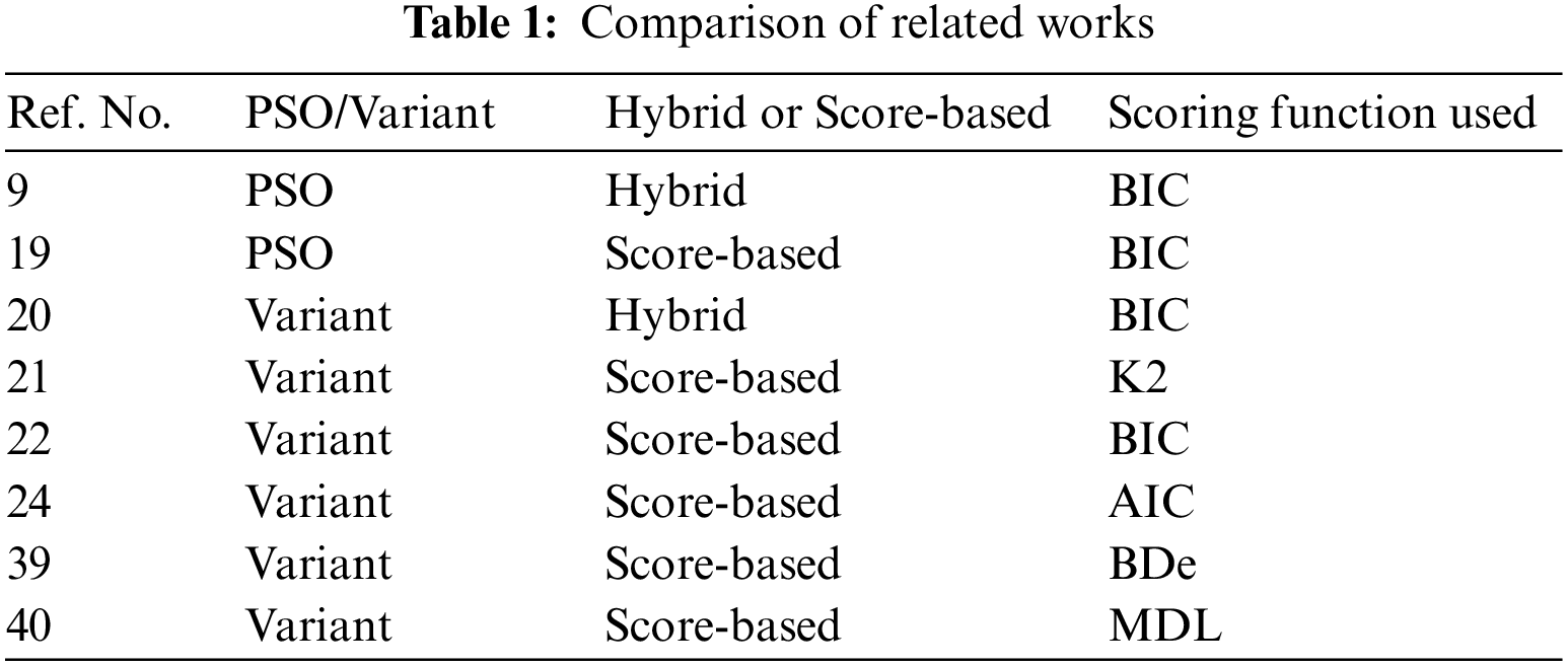
Generalized particle swarm optimization (GEPSO) [43] proposes variations in the PSO algorithm. It enhances the original PSO by integrating more terms (two) into the velocity update equation. The purpose of these terms is: to increase knowledge sharing and interrelations between particles, to diversify the swarm, and to enhance searching ability in unexplored areas of the search space. Table 1 shows the different methodologies that fellow researchers have used. We can see that different scoring functions have been used that include Bayesian information criterion (BIC), K2, Akaike information criterion (AIC), Minimum description length (MDL), and Bayesian Dirichlet equivalent (BDe).

In this paper, we have made two contributions: firstly, we discretize GEPSO and use it to learn BN structure (the discretization was inspired by [9,31]). Secondly, we propose a novel velocity update procedure that optimizes the Bayesian network-generalized particle swarm optimization (BN-GEPSO) search process.

3  Brief Introduction to Bayesian Networks

Two basic components that make a BN are a DAG denoted as DAG=G=(Nodes,Edges) and more than one table that describe CPTs. Because BN’s follow Markov property a CPT for a particular node shows the effect of parents on that node. An example of a bayesian network is provided in Fig. 1.

Figure 1: ASIA (lung cancer) Bayesian network

An edge that goes from node N1 to node N2 (denoted as N1→N2) means that node N1 is the cause (parent) of node N2. Non-appearance of an arrow tells that variable under observation does not depend on each other (marginal or conditional independence). Leveraging the Markov property, we can write the following, see Eq. (1) for a node B and its parents Pa(B):

P(B)=∏l=1nP(Bl|Pa(Bl))(1)

Score-Based Approach for BN Structure Learning

The aim of the score-based BN structure learning is to use the training dataset (D) to determine the network structure (T) having the best score see Eq. (2).

P(T|D)=P(T,D)P(D)=P(T,D)(2)

Since P(D) is independent of structure, P(T, D) is used as a scoring metric. There are different scoring metrics, but the one we will be using is the BIC score see Eq. (3).

BICscore(T|D)=∑u=1n∑v=1qu∑w=1ruMuvwlog(MuvwMuv)−12∑u=1nqu(ru−1)log(M)(3)

Here M represents samples in the dataset, n is the total number of nodes, ru is the possible values of uth node xu, qu the possible values of the parent node of xu, Muvw is the number of cases in which parent nodes of xu take vth value and xu take wth value and Muv the number of cases where parent nodes of xu take vth value.

4  Discretization of GEPSO

After selecting the scoring function, we apply GEPSO to search for the optimal solution. Since we are working on a discrete optimization problem, Discrete binary PSO coding is used where particle position is represented with a matrix (see Eq. (4)) having values {0,1} and velocity by a matrix (see Eq. (5)) having values {−1,0,1}. If n is the total number of nodes in the network, then:

Xnxn=[x1,1…x1,n−1x1,n⋮⋮⋱⋮xn−1,1…xn−1,n−1xn−1,nxn,1…xn,n−1xn,n](4)

Vnxn=[v1,1…v1,n−1v1,n⋮⋮⋱⋮vn−1,1…vn−1,n−1vn−1,nvn,1…vn,n−1vn,n](5)

Both these matrices have size n x n. Fig. 2 is an example of coding, i.e., from a DAG to a matrix.

Figure 2: Position “Node coding” example

The GEPSO formula is redefined to work in discrete space (using DBPSO). Refer to Eqs. (6) and (7):

Prtvelji=Prtvelji−1+(Pbposji−1−Prtposji−1)+(Gbposji−1−Prtposji−1)+(Pbposrandomi−1−Prtposji−1)+Pvelrandom(6)

Prtposji=Prtposji−1++Prtvelji(7)

where the terms used are j = Particle number, i = Iteration number, Prtvelji−1= Previous/initial velocity randomly initialized in the start, Prtvel = Particle velocity, Pbpos = Personal best position, Gbpos = Global best position, Prtpos = Particle position, Pbposrandomi−1 = Best position of randomly chosen particle till iteration i, Pvelrandom = Randomly generated velocity.

Pbposrandomi−1 term incorporates the knowledge of neighboring particles at every iteration, thus leading us toward good results and bringing variety to the search process. On the other hand, Pvelrandom term prevents the algorithm from getting stuck at local optima. Below are examples (see Figs. 3 and 4) showing how particle velocity is calculated using DBPSO, and how we update the position when we have velocity.

Figure 3: New velocity using subtraction

Figure 4: New position using addition

We update the personal and global best position as shown in Eqs. (8) and (9):

If(BIC(Prtposji)>BIC(Prtposji−1))(8)

thenPbposji=Prtposji

If(BIC(Pbposji)>BIC(Gbposji−1))

thenGbposji=Pbposji(9)

Velocity Update Procedure

In our research, we keep the position updated as it is, while we propose to use a selection method to update velocity. We define the five velocities shown in Eq. (6) as V1, V2, V3, V4, and V5. Where V1 is the previous/initial velocity and we obtain the others as follows: V2 by subtracting the personal best position from the previous position, V3 by subtracting the global best position from the previous position, V4 by subtracting a random particles personal best position from the previous position, finally V5 is the randomly generated velocity. For each velocity, first, we find out the corresponding position update by addition, then we calculate the BIC score of the new position (posn1 for V1 by using function BIC (input). This is shown in Eq. (10)

temp1=posn1+V1cyclecheckbic=BIC(temp1)(10)

After that, we save all BIC scores in an array and normalize the array by its sum (so that the outputs are between {0,1}. We sort the array (array = [a, b, c, d, e]) in ascending order (while doing so, we keep the velocity linked with array indexes, such that we know whether “a” corresponds to V1 or V2 and so on). To be unbiased a random number in the interval {0,1} and we pick the update velocity as in Eq. (11). Suppose that a, b, c, d, e belongs to V1, V2, and so on after sorting.

Ifa>r and Vupdate=V1ElseIfb>r and Vupdate=V2ElseIfc>r and Vupdate=V3ElseIfd>r and Vupdate=V4ElseVupdate=V5(11)

5  Proposed Methodology

In our proposed method, we get an initial DAG (initial structure) to generate PSO particles by combining the MMPC algorithm [34] with cross-relative average entropy (CRAE). Algorithm 1, describes a short pseudo code for obtaining candidate parents and children (CPC) of a node using MMPC, while Algorithm 2, describes the complete procedure.

MMPC algorithm takes the target node and dataset as input and outputs a set that consists of possible parents and children of the target node (this set is not constrained in our approach). The max-min heuristic outputs the maximum association achieved (maximum from all the minimum associations, given target node and CPC set) and the node that has this value. If this association value is greater than zero, we add that node to our CPC set. In the backward phase, we double-check our CPC set for false positives (if there is some node in CPC that can cause another node in CPC to be independent of the target variable when conditioned on it, we remove that (another) node).

After MMPC executes, we have an un-directed graph between the target node and its CPC, so we use CRAE (Eqs. (12) and (13)) to determine the edge direction. This results in a directed graph. Since BN is a DAG by definition, we remove cycles from the directed graph, making it a DAG.

For two variables Ai Aj, where |Ai| and |Aj| represent the count of values of the variables Ai and Aj. CRAE is given as follows:

CRAE(Aj→Ai)=∑i=1n∑j=1mp(ai,aj)logp(ai|aj)−∑i=1np(ai)logp(ai)|Ai|(12)

CRAE(Ai→Aj)=∑i=1n∑j=1mp(ai,aj)logp(aj|ai)−∑j=1mp(aj)logp(aj)|Aj|(13)

We perform two operations similar to those used in [8] i.e., adding new edges and reversing the edges randomly. To produce an initial population for PSO search and to diversify it. These operations will create cycles, so we remove them to ensure all particles are DAGs. Last but not least, PSO initial parameters are initialized along with position and velocity matrices, followed by the PSO search. During the search when we update the position, cycles might be created, so we remove them accordingly.

6  Experiments and Results

6.1 Experimental Setup

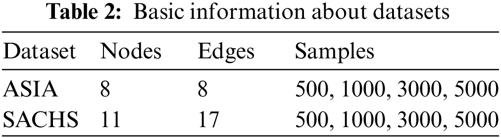
The experimental setup consisted of a personal laptop having the 10th generation Intel Core i7-10750H CPU with a frequency of 2.60 GHz, MS-Windows 10 (x64), and 16 GB RAM. The programming language used was Python (3.9.7), the main library used was “bnlearn,” and the compiler was “Spyder IDE 5.1.5” (Anaconda). The datasets used for testing our algorithm are the ASIA network (benchmark dataset), a small dataset that relates a visit to Asia and lung diseases, and the SACHS network, which consists of data regarding 11 proteins and phospholipids derived from immune system cells. For each dataset, we use four different sample sizes. These datasets are available in the bnlearn library. Samples are generated by using the python “bn.sampling” (model, number-samples) command. Table 2 gives basic details about the datasets used.

6.2 Evaluation Indicators

To evaluate our results, i.e., the learned Bayesian network structure we use the Mean BIC score of the final global best structure. BIC score outputs a negative value. The smaller the value, the better the result. In other words, BIC score furthest away from 0 is better. Time taken per iteration of PSO (TPI) in seconds and the total time taken for complete execution in minutes (TTT). Each experiment is repeated five times to get mean values. The number of particles is 100, total iterations for the GEPSO search procedure are 50.

6.3 Results

We have named our method BN-GEPSO, and we compare our results against discrete binary PSO (DBPSO) and LIPSO. DBPSO is in fact classic PSO, where we code position and velocity into matrices followed by adding the three velocity matrices and updating the position by the addition of velocity and position matrix. Table 3 displays the results for the ASIA dataset while Table 4 displays the performance for the SACHS dataset on DBPSO, BN-GEPSO, and LIPSO using sample sizes of 500,1000,3000, and 5000.

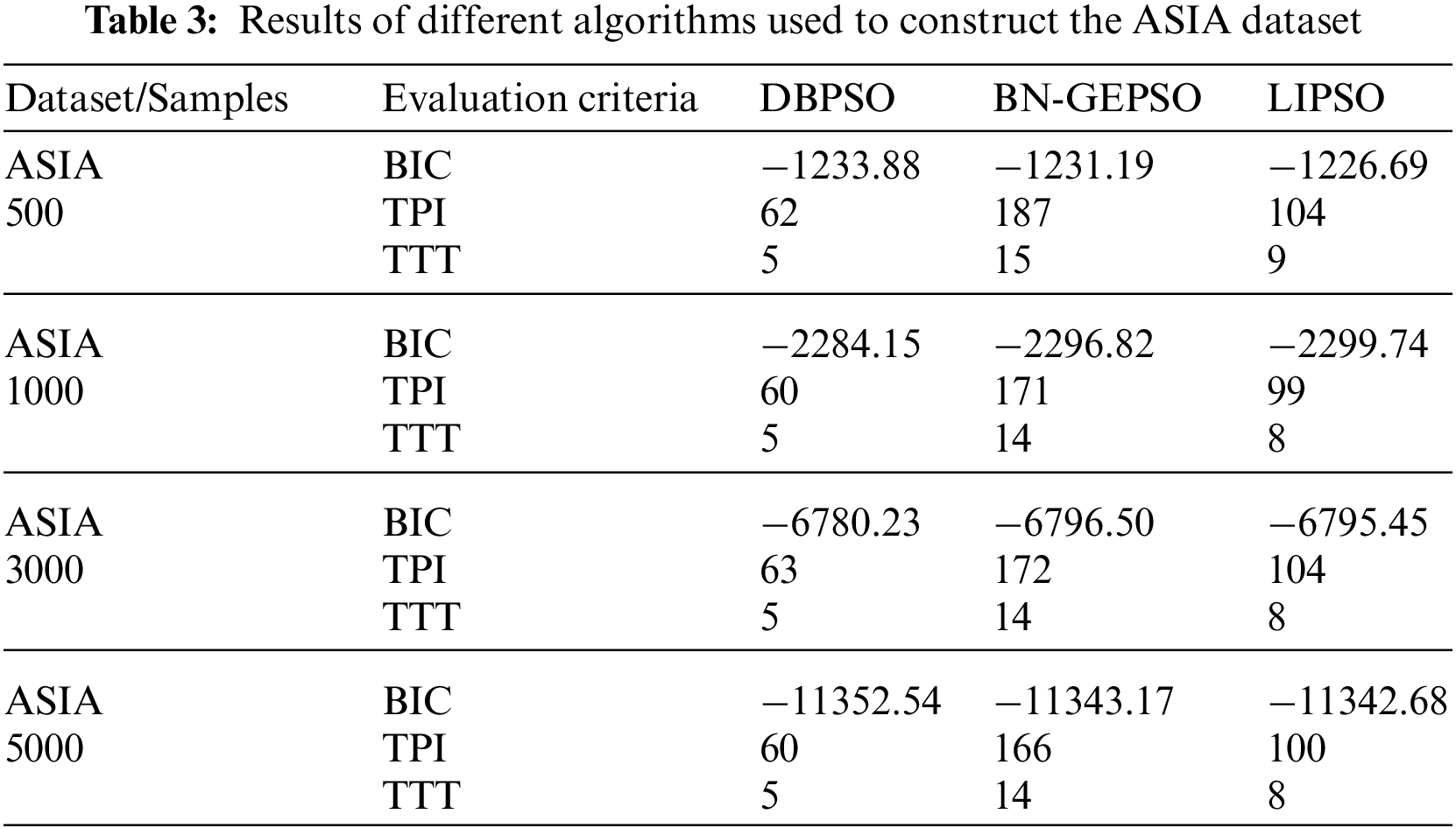
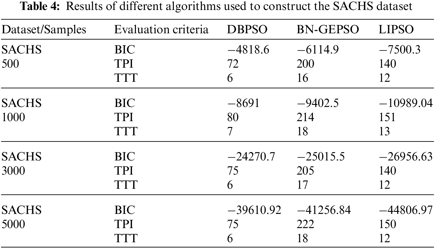
If we compare our BIC score with DBPSO and LIPSO on the ASIA dataset, we perform better than both of them. If in any case, we do lose, the margin is small. Contrary to that, on the SACHS dataset, LIPSO stays ahead of BN-GEPSO while using a dataset with more edges and nodes. A reason for this behavior is that LIPSO adds more information into the initial DAG using the mutual information step. In contrast, we don’t use this step. Another important behavior to see is that as the dataset gets bigger, we are outperforming the DBPSO algorithm, which was our target in this research, to prove that GEPSO works better than PSO while learning the BN structure.

Now, if we compare TTI and TTT terms we are losing here. The reason is that we have five velocity terms (PSO has three). Another reason is that we are not using any constraining step to limit the maximum number of CPC nodes for each target node.

While DBPSO does not have CPC and LIPSO constrains it to a maximum of 2. We did this to show how knowledge sharing in GEPSO is working. Note that the fourth term in GEPSO, which choose the random best position of a random particle, works to share information between particles. From our experiments, we can see that this information sharing is not as effective as using mutual information at the beginning phase before the CRAE step.

7  Conclusions

We have discretized GEPSO (a new generalized PSO algorithm) and used it to learn the Bayesian network (BN) structure. We name this Bayesian network generalized particle swarm optimization (BN-GEPSO). The discretization was inspired by discrete binary particle swarm optimization (DBPSO). BN-GEPSO uses the max min parent’s and children (MMPC) algorithm and crosses relative average entropy (CRAE) to generate an initial directed acyclic graph (DAG) structure. Then two operations of adding and reversing edges are performed to generate an initial population for GEPSO. Finally, GEPSO iterates, and we choose the best global solution as our output. We also proposed a way to update the velocity hence improving the search process. Experiments were performed on datasets of different sample sizes, which concluded that BN-GEPSO outperforms DBPSO as the complexity of the dataset increases. Future research directions include: reducing total time taken per iteration (TTI) and total time taken for complete execution (TTT) values by constraining candidate parents and children (CPC) set, applying this approach to continuous data (learning BN structure from continuous data, and instead of using our equations, the GEPSO paper is to be the reference. GEPSO has different parameters, weights, etc., which are not taken into consideration when discretizing. This means that we still have to fully unleash the power of this algorithm). This approach can also be extended towards time-based data as in dynamic Bayesian networks (where we work with data at different time slices), experimenting on large samples sizes and datasets by leveraging the parallel power of graphics processing units (GPUs), improving the velocity update procedure, application-based studies, for example, using BN-GEPSO for the analysis of disease, making an application for insurance companies to predict the risk of each customer to decide whether they are a good or bad fit (this approach will focus more on BN prediction, BN classification, and BN inference).

Acknowledgement: The authors extended their appreciation to the Deanship of Scientific Research at King Khalid University for funding this work through the Large Groups Project under grant number RGP.2/132/43. The authors express their gratitude to the editor and referees for their valuable time and efforts on our manuscript.

Funding Statement: Funds are available under the Grant Number RGP.2/132/43 at King Khalid University, Kingdom of Saudi Arabia.

Conflicts of Interest: The authors declare that they have no conflicts of interest to report regarding the present study.

References

1. F. V. Jensen and T. D. Nielsen, “Bayesian Networks and Decision Graphs,” 2nd ed., New York, USA: Springer, pp. 23–50, 2001. [Google Scholar]

2. R. He, X. Li, G. Chen, Y. Wang, S. Jiang et al., “A quantitative risk analysis model considering uncertain information,” Process Safety and Environmental Protection, vol. 118, no. 5, pp. 361–370, 2018. [Google Scholar]

3. K. Sachs, O. Perez, D. Pe’er, D. A. Lauffenburger and G. P. Nolan, “Causal protein-signaling networks derived from multiparameter single-cell data,” Science, vol. 308, no. 5721, pp. 523–529, 2005. [Google Scholar] [PubMed]

4. W. Li, P. Zhang, H. Leung and S. Ji, “A novel qos prediction approach for cloud services using bayesian network model,” IEEE Access, vol. 6, pp. 391–1406, 2017. [Google Scholar]

5. M. Hafiz Mohd Yusof, A. Mohd Zin and N. Safie Mohd Satar, “Behavioral intrusion prediction model on bayesian network over healthcare infrastructure,” Computers, Materials & Continua, vol. 72, no. 2, pp. 2445–2466, 2022. [Google Scholar]

6. S. Li, S. Chen and Y. Liu, “A method of emergent event evolution reasoning based on ontology cluster and bayesian network,” IEEE Access, vol. 7, pp. 15 230–15 238, 2019. [Google Scholar]

7. A. A. El-Saleh, A. Alhammadi, I. Shayea, A. Azizan and W. Haslina Hassan, “Mean opinion score estimation for mobile broadband networks using bayesian networks,” Computers, Materials & Continua, vol. 72, no. 3, pp. 4571–4587, 2022. [Google Scholar]

8. K. Murphy, “An introduction to graphical models,” 2001. [Online]. Available: http://www2.denizyuret.com/ref/murphy/intro_gm.pdf [Google Scholar]

9. K. Liu, Y. Cui, J. Ren and P. Li, “An improved particle swarm optimization algorithm for bayesian network structure learning via local information constraint,” IEEE Access, vol. 9, pp. 40 963–40 971, 2021. [Google Scholar]

10. B. Andrews, J. Ramsey and G. F. Cooper, “Scoring bayesian networks of mixed variables,” International Journal of Data Science and Analytics, vol. 6, no. 1, pp. 3–18, 2018. [Google Scholar] [PubMed]

11. E. S. Adabor, G. K. Acquaah-Mensah and F. T. Oduro, “Saga: A hybrid search algorithm for bayesian network structure learning of transcriptional regulatory networks,” Journal of Biomedical Informatics, vol. 53, no. 4, pp. 27–35, 2015. [Google Scholar] [PubMed]

12. Y. Jiang, Z. Liang, H. Gao, Y. Guo, Z. Zhong et al., “An improved constraint-based bayesian network learning method using gaussian kernel probability density estimator,” Expert Systems with Applications, vol. 113, no. 6, pp. 544–554, 2018. [Google Scholar]

13. P. Spirtes, C. N. Glymour and R. Scheines, “Causation, prediction, and search,” 2nd ed., London, UK: The MIT press, pp. 78–97, 2000. [Google Scholar]

14. X. Xie and Z. Geng, “A recursive method for structural learning of directed acyclic graphs,” The Journal of Machine Learning Research, vol. 9, pp. 459–483, 2008. [Google Scholar]

15. A. L. Madsen, F. Jensen, A. Salmer´on, H. Langseth and T. D. Nielsen, “A parallel algorithm for bayesian network structure learning from large data sets,” Knowledge-Based Systems, vol. 117, no. 3, pp. 46–55, 2017. [Google Scholar]

16. X. Sun, C. Chen, L. Wang, H. Kang, Y. Shen et al., “Hybrid optimization algorithm for bayesian network structure learning,” Information-an International Interdisciplinary Journal, vol. 10, no. 10, pp. 294, 2019. [Google Scholar]

17. S. Acid and L. M. De Campos, “A hybrid methodology for learning belief networks: Benedict,” International Journal of Approximate Reasoning, vol. 27, no. 3, pp. 235–262, 2001. [Google Scholar]

18. M. Chickering, D. Heckerman and C. Meek, “Large-sample learning of bayesian networks is np-hard,” Journal of Machine Learning Research, vol. 5, pp. 1287–1330, 2004. [Google Scholar]

19. X. Liu and X. Liu, “Structure learning of bayesian networks by continuous particle swarm optimization algorithms,” Journal of Statistical Computation and Simulation, vol. 88, no. 8, pp. 1528–1556, 2018. [Google Scholar]

20. B. Sun, Y. Zhou, J. Wang and W. Zhang, “A new pc-pso algorithm for bayesian network structure learning with structure priors,” Expert Systems with Applications, vol. 184, no. 4, pp. 115237, 2021. [Google Scholar]

21. J. Wang and S. Liu, “A novel discrete particle swarm optimization algorithm for solving bayesian network structures learning problem,” International Journal of Computer Mathematics, vol. 96, no. 12, pp. 2423–2440, 2019. [Google Scholar]

22. L. Yang, J. Wu and F. Liu, “Bayesian network structure learning based on modified particle swarm optimisation,” International Journal of Information and Communication Technology, vol. 8, no. 1, pp. 112–121, 2016. [Google Scholar]

23. S. Gheisari and M. R. Meybodi, “Bnc-pso: Structure learning of bayesian networks by particle swarm optimization,” Information Sciences, vol. 348, no. 3, pp. 272–289, 2016. [Google Scholar]

24. S. Aouay, S. Jamoussi and Y. BenAyed, “Particle swarm optimization based method for bayesian network structure learning,” in 5th Int. Conf. on Modeling, Simulation and Applied Optimization (ICMSAO), Hammamet, Tunisia, pp. 1–6, 2013. [Google Scholar]

25. C. Contaldi, F. Vafaee and P. C. Nelson, “Bayesian network hybrid learning using an elite-guided genetic algorithm,” Artificial Intelligence Review, vol. 52, no. 1, pp. 245–272, 2019. [Google Scholar]

26. S. Lee and S. B. Kim, “Parallel simulated annealing with a greedy algorithm for bayesian network structure learning,” IEEE Transactions on Knowledge and Data Engineering, vol. 32, no. 6, pp. 1157–1166, 2019. [Google Scholar]

27. C. Yang, H. Gao, X. Yang, S. Huang, Y. Kan et al., “Bnbeeepi: An approach of epistasis mining based on artificial bee colony algorithm optimizing bayesian network,” in IEEE Int. Conf. on Bioinformatics and Biomedicine (BIBM), San Diego, CA, USA, pp. 232–239, 2019. [Google Scholar]

28. X. Zhang, Y. Xue, X. Lu and S. Jia, “Differential-evolution-based coevolution ant colony optimization algorithm for bayesian network structure learning,” Algorithms, vol. 11, no. 11, pp. 188, 2018. [Google Scholar]

29. S. W. Kareem, F. Q. Alyousuf, K. Ahmad, R. Hawezi and H. Q. Awla, “Structure learning of bayesian network: A review,” Qalaai Zanist Journal, vol. 7, pp. 956–975, 2022. [Google Scholar]

30. X. Wang, H. Ren and X. Guo, “A novel discrete firefly algorithm for Bayesian network structure learning,” Knowledge-Based Systems, vol. 242, p. 108426, 2022. [Google Scholar]

31. H. Xing-Chen, Q. Zheng, T. Lei and S. Li-Ping, “Learning bayesian network structures with discrete particle swarm optimization algorithm,” in IEEE Symp. on Foundations of Computational Intelligence, Honolulu, Hawaii, pp. 47–52, 2007. [Google Scholar]

32. X. C. Heng, Z. Qin, X. H. Wang and L.-P. Shao, “Research on learning bayesian networks by particle swarm optimization,” Information Technology Journal, vol. 5, no. 3, pp. 540–545, 2006. [Google Scholar]

33. T. Wang and J. Yang, “A heuristic method for learning bayesian networks using discrete particle swarm optimization,” Knowledge and Information Systems, vol. 24, no. 2, pp. 269–281, 2010. [Google Scholar]

34. I. Tsamardinos, L. E. Brown and C. F. Aliferis, “The max-min hillclimbing bayesian network structure learning algorithm,” Machine Learning, vol. 65, no. 1, pp. 31–78, 2006. [Google Scholar]

35. P. Spirtes and C. Meek, “Learning bayesian networks with discrete variables from data,” in Conf. on Knowledge Discovery and Data Mining (KDD), Montreal, Canada, vol. 1, pp. 294–299, 1995. [Google Scholar]

36. E. Lantz, S. Ray and D. Page, “Learning bayesian network structure from correlation-immune data,” arXiv preprint arXiv: 1206. 5271, 2012. [Google Scholar]

37. J. Kennedy and R. Eberhart, “Particle swarm optimization,” in Proc. of ICNN’95-Int. Conf. on Neural Networks, Perth, WA, IEEE, vol. 4, pp. 1942–1948, 1995. [Google Scholar]

38. E. Brenner and D. Sontag, “Sparsityboost: A new scoring function for learning bayesian network structure,” arXiv preprint arXiv: 1309. 6820, 2013. [Google Scholar]

39. Q. Zhang, Z. Li, C. Zhou and X. Wei, “Bayesian network structure learning based on the chaotic particle swarm optimization algorithm,” Genetics and Molecular Research, vol. 12, no. 4, pp. 4468–4479, 2013. [Google Scholar] [PubMed]

40. X.-L. Li and X.-D. He, “A hybrid particle swarm optimization method for structure learning of probabilistic relational models,” Information Sciences, vol. 283, no. 1, pp. 258–266, 2014. [Google Scholar]

41. C. Chow and C. Liu, “Approximating discrete probability distributions with dependence trees,” IEEE Transactions on Information Theory, vol. 14, no. 3, pp. 462–467, 1968. [Google Scholar]

42. C. Xiaoyu and L. Baoning, “Bayesian network structure learning based on small sample data,” in 6th Int. Conf. on Robotics and Automation Engineering (ICRAE), Guangzhou, China, pp. 393–397, 2021. [Google Scholar]

43. D. Sedighizadeh, E. Masehian, M. Sedighizadeh and H. Akbaripour, “Gepso: A new generalized particle swarm optimization algorithm,” Mathematics and Computers in Simulation, vol. 179, no. 2, pp. 194–212, 2021. [Google Scholar]