A Convolutional Neural Network Model for Wheat Crop Disease Prediction

1  Introduction

Wheat is the globally most consumed food crop. It fulfills a significant portion of the daily energy requirements of the human body [1]. The genetic components of wheat (notably proteins, fiber, and vitamins) increase its consumption worldwide [2,3]. According to USDA foreign agricultural service report [4], more than 700 million metric tons of wheat have been produced globally in the last nine years, which is still less than its demand (shown in Fig. 1). The wheat demand is increasing daily, whereas its production is severely affected by natural disasters, climate change, war, and crop diseases. Among these challenges, wheat crop disease is of significant importance. If it is not prevented, it can be more destructive than its counterparts. The timely diagnosis and detection of wheat diseases are not only crucial for their prevention, but can also increase their production yield to boost the national economy. There are various techniques for detecting crop diseases such as microscopic techniques and manual visualization. However, these techniques are time extensive and error-prone due to human error factors. Thus, the researchers introduced alternative automatic techniques to identify crop diseases [5].

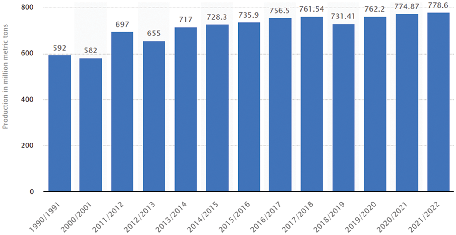
Figure 1: Global annual wheat production from 2011/2012 to 2021/2022 (million metric tons) [4]

The advancement in computer vision and machine learning increased the research interest in image-based automated detection systems for wheat diseases [6–8]. These techniques are adequate replacements of the time expensive and lab extensive diagnoses [9]. These techniques need standard equipment such as cameras, mobile phones, and commonly used storage to perform disease detection and classification. These techniques are subjective and focus on the specific task and require domain expert knowledge for feature extraction. Additionally, these techniques work ideally in a practical experimental setup.

The literature showed that most of the time, researchers used the standard dataset to evaluate their machine learning models. Although the machine learning models have achieved promising results on standard datasets but in-fields captured images have their own challenges. As mentioned in [10], those challenges include (a) complex background of the image, (b) challenging lighting effects, (c) fuzzy boundaries of the disease, (d) multiple diseases in a single image, (e) similar characteristics of different diseases, (f) distinctive characteristics for the same disease according to its shape and stage. Thus, in-field wheat disease detection is still a challenging task.

In this paper, the contribution is three-fold. First, this paper proposes a simple and lightweight CNN-based model that can also be used for smartphones in the future. Second, it will be fast enough to predict wheat disease in real-time. Third, it can increase the production yield by timely detecting in-field wheat crop disease. The rest of the paper is organized as follows. The next section provides a review of the existing literature in this field. Then Section 3 provides the proposed methods and materials, followed by results and discussion in Section 4, and finally, the conclusion and future work dimensions are presented in Section 5.

2  Related Work

Many CNN models have already been proposed for image-based crop disease prediction and classification. The proposed work in [11] introduced a deep learning model based on weekly supervised learning. The work includes training the model on onion crops with six categories of symptoms and using the activation map to localize diseases. The trained model used image-level annotation to detect and classify crop diseases. This model effectively identified the symptoms of onion crops diseases. The work in [12] used CNN to detect diseases from wheat images and use visualization methods to understand the learning behavior of these models. They used the CRAW dataset, containing 1163 images, divided into unhealthy and healthy classes. Another model, CNN-F5 [13], found a more representative subset of features for the original data set. This model maintains its high accuracy of 90.20% by training the 60-channel features.

In the work of [14], the researchers used hyperspectral imaging technology and the random forest method to analyze the reflectance spectrum of healthy and unhealthy wheat crop data. The characteristic wavelengths selected by random forest are 600 nm for late-stage seed germination, 800 nm for early-stage germination and 1400 nm for joint-stage germination that combines flowering and grouting. The work of [15] also provides a comprehensive overview of wheat rust disease research in India. Efforts are being made worldwide to monitor rust, identify the types of rust pathways and evaluate the rust resistance of wheat germ pulp. The responsible determination of early growth and rust-free varieties proved to be an effective strategy for managing its eradication [15]. However, efforts are still continued to eradicate wheat rust diseases. The rust and genomic methods are used to break down barriers that undermine performance and prevent wheat diseases. The critical factors for effective wheat disease prevention management require the effective classification of rusty stems from wheat, classification of sources of resistance and usage of preventive measures against them.

The works of [16,17] developed a CNN model to classify the diseases in maize. In other studies conducted in [18,19], the researchers identified diseases in apple trees. In [20], the authors presented a CNN model to detect the ‘black sigatoka’ and ‘black speckled’ diseases in banana plants. The work of [21] presented CNN models, trained on a dataset of 5632 images, to predict tea diseases. This work used GoogleNet, MCT and AlexNet models. Similarly, the work of [22] developed a CNN model for the detection of diseases in cucumber plants. The research works of [23,24] have classified the ‘fusarium wilt’ disease for radish plants. Furthermore, the authors of [25] had given a dataset of multiple plants and used CNN model that provided good accuracy of 95% for pepper plant disease detection. In Reference [26], the researchers used CNN architecture for disease classification in grapes. The authors of [27] have developed their dataset and introduced a CNN model for predicting soybean plant diseases.

Table 1 highlights the strengths and weaknesses of commonly used neural network models for crop disease prediction. These strengths and weaknesses are helpful in selecting the appropriate model according to the classification dataset.

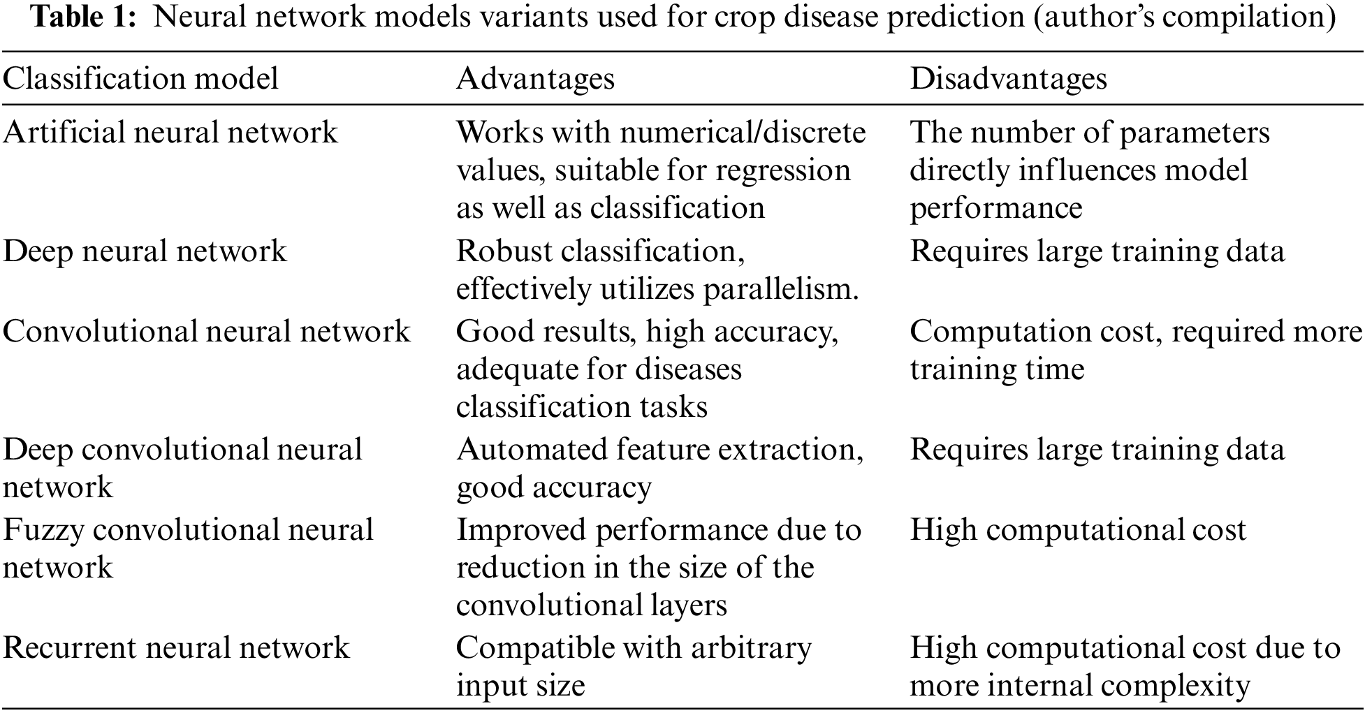
As evident from Table 1, the proposed model for this research is a variant of CNN and it achieves the goal of good classification with a small number of internal layers.

3  Proposed Methodology

This section explains the proposed methodology, of this work, in detail by describing the captured dataset, proposed model architecture, experimental environment, and employed performance evaluation metrics.

3.1 Dataset

The dataset was collected from the wheat fields in the district Kotli of Azad Kashmir (Pakistan). All the dataset images were captured using different models of mobile phones, including Infinix Hot8, Samsung J7 Prime, Samsung J7 Pro, and iPhone 8. All images were taken at the random angles and locations from the overall field. The total captured images were 3750. All the images were reevaluated, and the faulty images were removed. The remaining 1567 images were annotated manually by the field experts. Finally, 450 images were selected for the experiments based on the consensus in the opinion of experts. In the final dataset, 225 images belong to the healthy class and 225 to the unhealthy class. Some sample images are shown in Fig. 2a whereas, Fig. 2b shows specifically unhealthy images of the dataset.

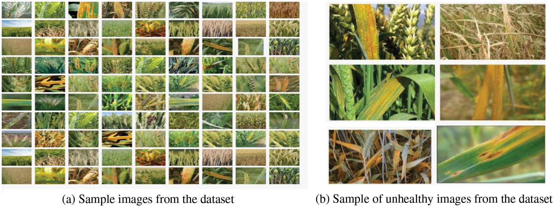
Figure 2: Sample healthy and unhealthy images from the captured dataset

3.2 Model Architecture

CNN is a deep neural network model trained through a supervised learning mechanism. It processes data effectively in the form of vectors and matrices. The basic structure of the CNN consists of an input layer, an output layer, and a sequence of hidden layers that map the input to the output. These layers work on the interconnection of the network and shared weight associated with internal neurons.

The convolutional layer uses the concept of the chain rule of derivatives. This rule shows how the slight change in x affects the change in y and z. It uses the principle of partial derivatives that compose that minor change in x (Δx) first make a slight change in y (Δy) by ∂x/∂y. Similarly, Δy brings changes in Δz. Combining both equations produces Δy/Δx and Δz/Δx. Extending the chain rule of derivatives for an input unit xi, jl give the general equation as shown in Eq. (1).

xi,jl=∑p=0m−1∑q−1m−1ωpqy(i−p)(j−q)l−1(1)

Once the convolutional layer computes error rate E, the partial derivative of E is calculated at the current layer, as shown in Eq. (2).

∂E∂xpql=∂E∂ypql∂ypql∂xpql=∂E∂ypql∂∂xpql(σ(xpql)=∂E∂ypqlσ′(xpql)(2)

It helps in the calculation of the backward propagation at the previous layer. After the convolutional layer transformation in the feature maps, the max-pooling layer tries to retrieve the high-order features from the features for robustness. It reduces the input of the specific location to a single value that achieves the goal of high order features extractions. The max-pool equation is presented in Eq. (3).

yi,j,kl= p,qmaxxi.j−p,k+ql−1(3)

where xi.j−p,k+ql−1 represent l−1 layer ith feature map at j and k location and p,q are vertical and horizontal indices. The max-pooling layer uses a sliding window for the extraction of non-overlapping blocks. These blocks are then converted to single values to get the high-order features. The final layers, before the output layer, are fully connected layers. These layers calculate the weighted sum of the preceding layers to convert all values for classification and prediction which is the task of the final output layer. The equation of the fully connected layer is presented in Eq. (4).

xl=wlxl−1+bl(4)

where the xl is the output of the fully connected layer, xl−1 represents the previous fully connected layers, wl is the weighted coefficient, and bl is the bias of the layer. The convolutional and hidden layers use the ReLU (Rectifier Linear Unit) activation functions as , calculated through the formula given in Eq. (5). The output layer uses SoftMax whose formula is given in Eq. (6).

R(x)={0,if x≤0x,otherwise}(5)

Soft(xi)=exi∑j=1nexj(6)

The proposed CNN model comprises three convolutional layers, three pooling layers, three fully connected layers, and an input and output layer. The detailed model architecture is shown in Fig. 3.

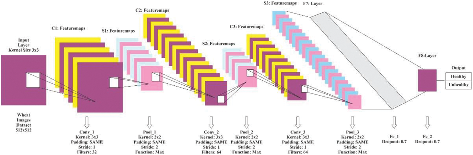
Figure 3: Proposed CNN model architecture

The three convolutional layers use 16, 32, and 64 filters. Every filter has a 3 × 3 kernel size and the strides are set to 1 for all convolutional layers. However, the kernel size for the pooling layers is set to 2 × 2 with stride 2. The learning rate was initially set to 0.001, while the input image resolution was set to 200 × 200 pixels. As described before, the ReLU activation function is utilized in the convolutional layers, and the SoftMax function is utilized in the pooling layers. In all layers of the model, the padding was set to default. The experimentation through this trained proposed model is explained in detail in the next section. It has proved that the combination of the hyper-parameters of the proposed CNN model, its filers, max-pooling layers, and fully connected layers performed better in disease classification of the wheat crop in in-field images.

3.3 Experimental Environment

The experimentation was conducted using Google Colab with the default setting for python with GPU The JPEG files of dataset images contained raw color photos of both classes of healthy and unhealthy wheat crops. These images are divided into two directories. Due to the relatively small dataset size, the experiments were carried out multiple times to check for model overfitting issues. In addition, the three variants of the dataset, created according to the dataset spilt, are used to evaluate the model. All the variants contained non-overlapping images.

3.4 Performance Evaluation Measures

The performance evaluation is made through the measures of accuracy, recall, precision, and f1 which are the standard metrics used for classification. The equations for these performance measures are shown in Eqs. (7)–(10). In addition, the class-wise performance evaluation is also used to measure the class_level performance of the classifiers.

Accuracy=TP+TNTP+TN+FP+FN(7)

Recall=TPTP+FN(8)

Precision=TPTP+FP(9)

f1=2(Recall ∗ PrecisionRecall+Precision)(10)

4  Results and Discussion

4.1 Model Training on Different Dataset Variants

The proposed convolutional neural network is trained on multiple versions of datasets. Figs. 4–6 highlight the model loss for training and validation on the split dataset versions represented by mnemonics s1, s2 and s3 where s1 represents (70, 15, 15), s2 represents (75, 15, 10) and s3 represents (80, 10, 10) for the split ratio of training, validating, and testing data respectively.

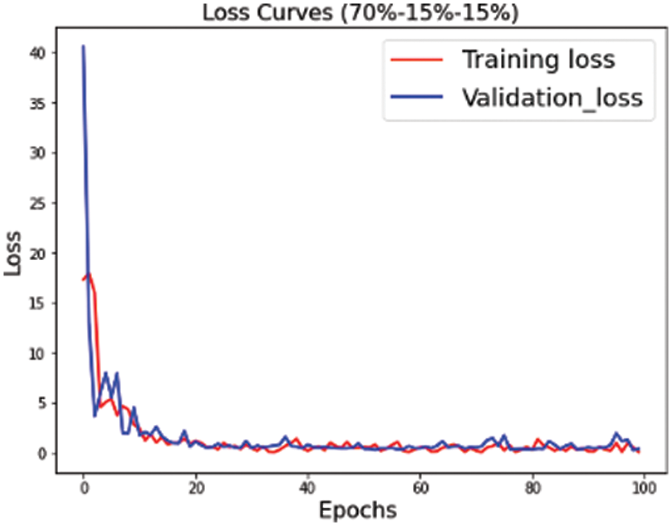
Figure 4: Training validation loss for the s1 (70, 15, 15) dataset split

Figure 5: Training validation loss for the s2 (75, 15, 10) dataset split

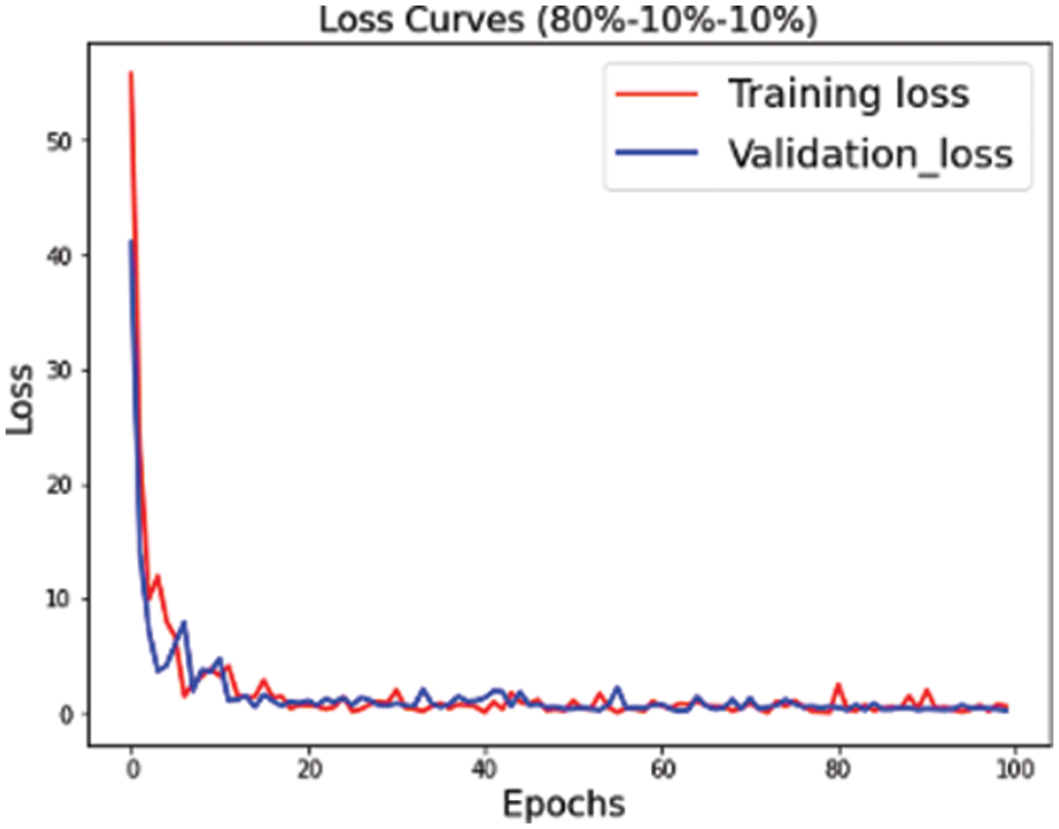
Figure 6: Training validation loss for s3 (80, 10, 10) dataset split

Figs. 7–9 represent the accuracy curve for the different experimental setups. The accuracies for the s1 (70, 15, 15) and s2 (75, 15, 10) dataset splits have higher fluctuation bands than the s3 (80, 10, 10) dataset split. The training accuracy band for Fig. 7 is between 30% and 100%, while for Fig. 8, it is between 20% and 100%. The larger band in accuracy for different epochs negatively affects the overall average score of the model. However, when the training size was increased to 80% of the dataset, the accuracy improved for both training and test datasets. The accuracy for validation, on the other hand, is relatively better than the training for s1, s2, and s3.

Figure 7: Training and validation accuracy for s1 dataset split

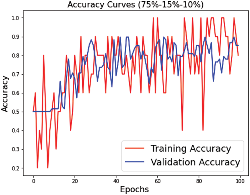
Figure 8: Training and validation accuracy for s2 dataset split

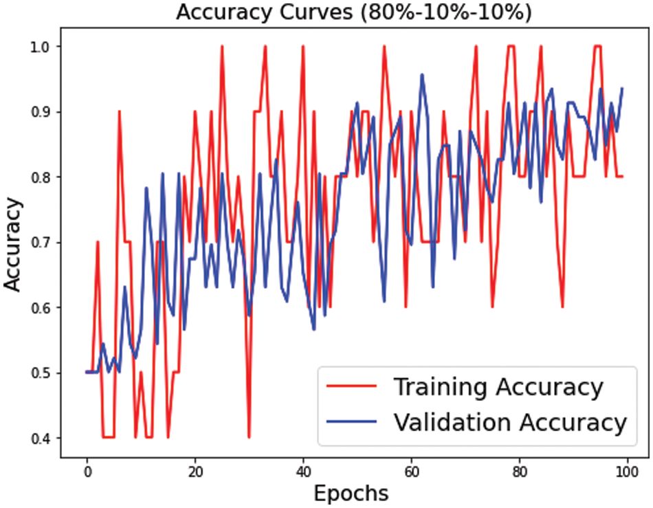
Figure 9: Training and validation accuracy for s3 dataset split

4.2 Model Testing on Different Dataset Variants

The model performed relatively better on the test datasets. The obtained confusion matrices of all three variants of dataset splits (s1, s2 and s3) are presented in Figs. 10–12. Fig. 10 shows the performance for the s1 dataset split, where it has shown better performance for healthy images where the prediction accuracy was 97%. Still, it was not good in predicting unhealthy images as it had shown merely 71% accuracy for them. Thus, negatively impacting the overall performance. On the other hand, Fig. 11 is giving a relatively better performance with 87% and 83% accurate results for healthy and unhealthy classes for the s2. In the s3 with 80% training data, the performance is best among all three data splitting schemes.

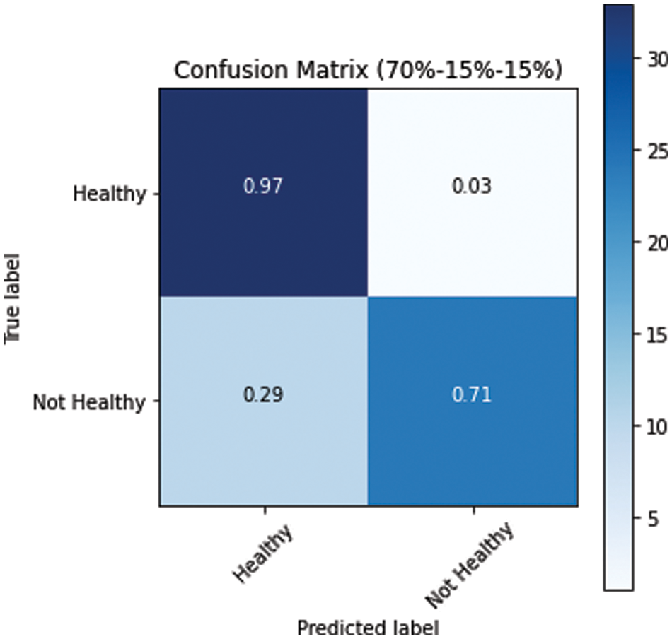
Figure 10: Confusion matrix for s1 dataset split

Figure 11: Confusion matrix for s2 dataset split

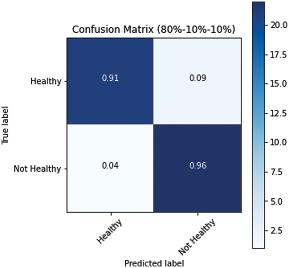
Figure 12: Confusion matrix for s3 dataset split

Besides the accuracy of the models, the classifier’s performance is also evaluated through precision, recall and f1 measures. It ensures not only the overall performance but also the prediction accuracy on both class levels. Table 2 presents these measures for all three dataset variants at each class level.

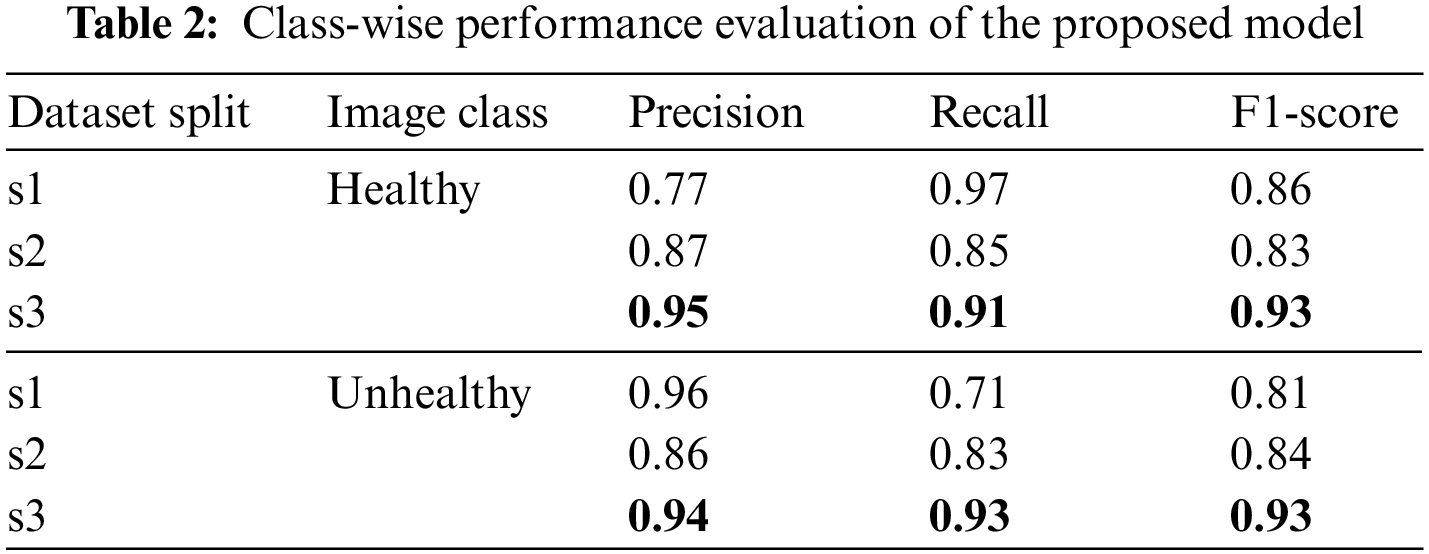
The above results have shown that larger training dataset results are better in all measures for both classes, where the smaller training set’s performance is relatively lower. Table 3 presents the weighted average results for both classes. In the combined results, all the numbers are in the acceptable range as all results are higher than 84%. However, the results of the third data split, s3 of (80, 10, 10) ratio, are highest with 0.94 precision, 0.93 recall, 0.93 f1 scores and 93% accuracy.

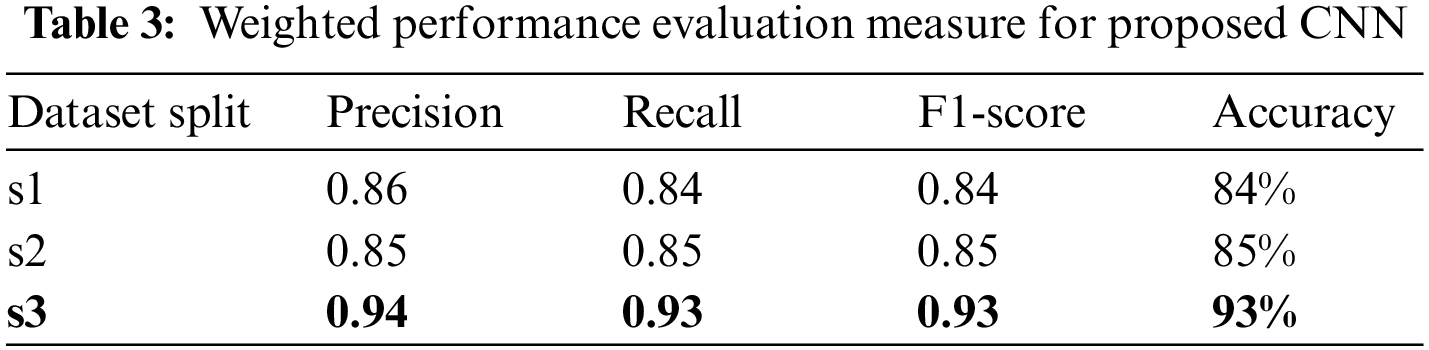
Table 4 provides a comparative analysis of state-of-the-art works for crop disease detection and classification. The table shows that the proposed model performed better than the majority of the models of state-of-the-art. However, the performance of the proposed model is best and almost similar to [28] in terms of accuracy.

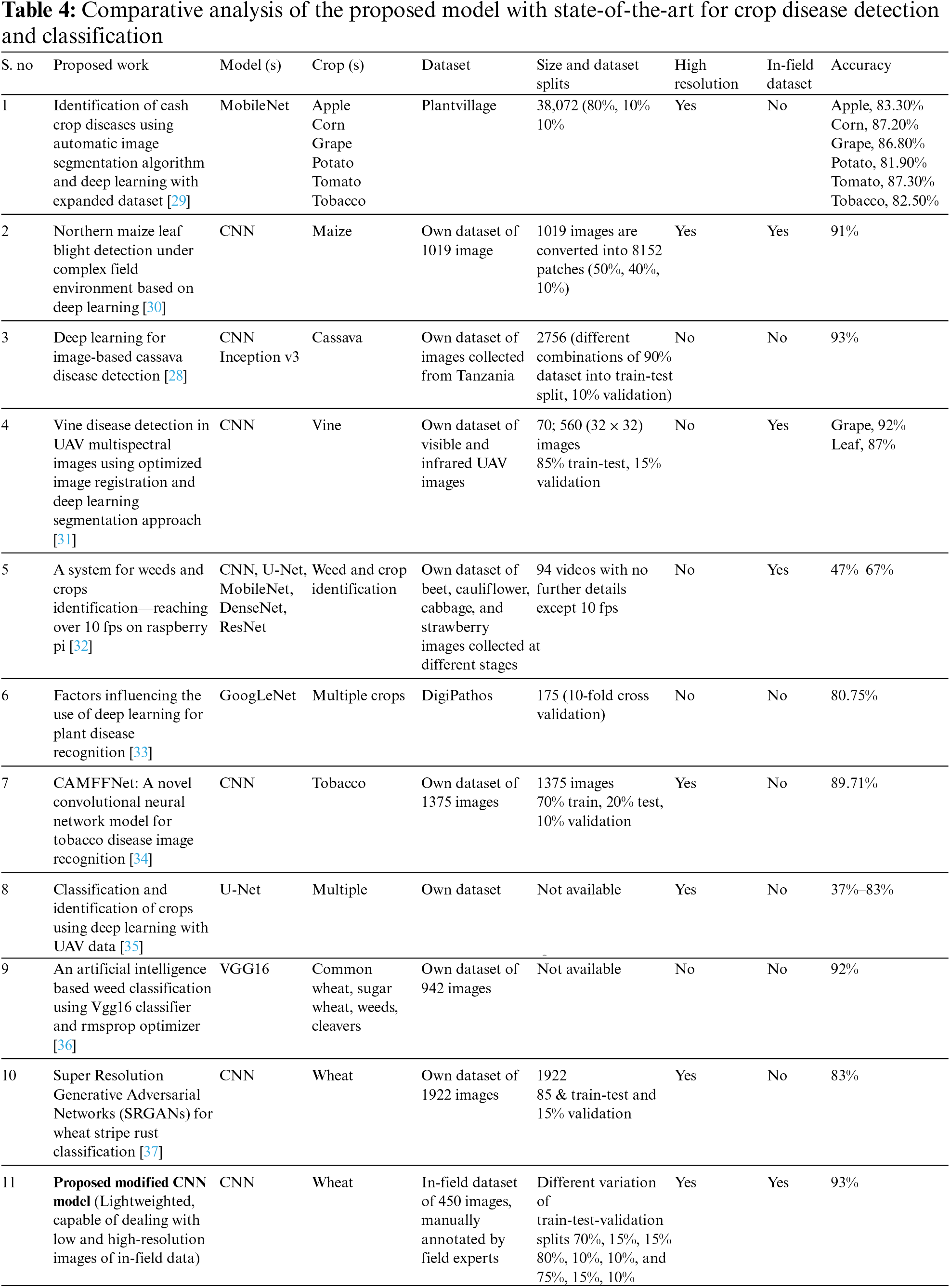
Table 4 highlights that only the researchers in [30] used both the in-field and high-resolution images. However, despite high computation, the reported accuracy is 91%. The authors in [28] reported a 93% accuracy, but they were using low-resolution data. There is a debate that training set size is positively correlated with accuracy. Some recent researchers [38,39] support this claim. On the other side, the researcher in [40] claimed 90% accuracy with 40% training dataset, by experimenting with 468 models. Therefore, the proposed modified CNN model is extensively evaluated on different variants of the dataset, and it was concluded that a higher number of images produces higher accuracy in the plant disease dataset.

5  Conclusion and Future Work

This research includes collecting images dataset from wheat fields of district Kotli of Azad Kashmir in Pakistan. These images are captured through mobile phones including Infinix Hot8, Samsung J7 Prime, Samsung J7 Pro and iPhone 8. The collected dataset is annotated by experts in two classes (healthy and unhealthy). A modified CNN model is proposed that is trained on the captured real dataset. The proposed model has shown the best results with 93% accuracy.

The fundamental challenge faced during the proposed research was the annotation, and validation from human expert; hence the dataset was limited to 450 images. However, in the future, it is planned to collect larger dataset of in-field images and annotate them for refined experimentation. However, data augmentation may also be utilized to enhance the existing datasets. In the future, it is planned to capture images through drones to capture a larger area of wheat fields to collect a larger dataset. The authors also planned to develop web services to provide online results to the farmers. Furthermore, in the future, the wheat crop images dataset is planned to cover multiple diseases, and it is planned to extend current work for multiple classifications and to predict different types of wheat crop diseases from their images.

Funding Statement: This work is funded by the University of Jeddah, Jeddah, Saudi Arabia (www.uj.edu.sa) under Grant No. UJ-21-DR-135. The authors, therefore, acknowledge the University of Jeddah for technical and financial support.

Conflicts of Interest: The authors declare that they have no conflicts of interest to report regarding the present study.

References

1. N. Poole, J. Donovan and O. Erenstein, “Agri-nutrition research: Revisiting the contribution of maize and wheat to human nutrition and health,” Food Policy, vol. 100, pp. 101976, 2021. [Google Scholar] [PubMed]

2. S. C. Bhardwaj, G. P. Singh, O. P. Gangwar, P. Prasad and S. Kumar, “Status of wheat rust research and progress in rust management-Indian context,” Agronomy, vol. 9, no. 12, pp. 892, 2019. [Google Scholar]

3. D. Zhang, Q. Wang, F. Lin, X. Yin, C. Gu et al., “Development and evaluation of a new spectral disease index to detect wheat fusarium head blight using hyperspectral imaging,” Sensors, vol. 20, no. 8, pp. 2260, 2020. [Google Scholar] [PubMed]

4. M. Shahbandeh, Global wheat production, 2022. [Online]. Available: https://www.statista.com/statistics/267268/production-of-wheat-worldwide-since-1990/ [Google Scholar]

5. J. Boulent, S. Foucher, J. Theau and P. L. St-Charles, “Convolutional neural networks for the automatic identification of plant diseases,” Front. Plant Sci., vol. 10, pp. 1–16, 2019. [Google Scholar]

6. V. K. Vishnoi, K. Kumar and B. Kumar, “Plant disease detection using computational intelligence and image processing,” Journal of Plant Diseases and Protection, vol. 128, no. 1, pp. 19–53, 2021. [Google Scholar]

7. M. Arya, K. Anjali and D. Unni, “Detection of unhealthy plant leaves using image processing and genetic algorithm with arduino,” in Proc. 2018 Int. Conf. on Power, Signals, Control and Computation (EPSCICON), Thrissur, India, pp. 1–5, 2018. [Google Scholar]

8. I. Hernández, S. Gutiérrez, S. Ceballos, F. Palacios, S. L. Toffolatti et al., “Assessment of downy mildew in grapevine using computer vision and fuzzy logic. Development and validation of a new method,” OENO One, vol. 56, no. 3, pp. 41–53, 2022. [Google Scholar]

9. J. Liu and X. Wang, “Plant diseases and pests detection based on deep learning: A review,” Plant Methods, vol. 17, no. 1, pp. 22, 2021. [Google Scholar] [PubMed]

10. A. Sinha and R. S. Shekhawat, “Review of image processing approaches for detecting plant diseases,” IET Image Processing, vol. 14, no. 8, pp. 1427–1439, 2020. [Google Scholar]

11. Y. Borhani, J. Khoramdel and E. Najafi, “A deep learning based approach for automated plant disease classification using vision transformer,” Scientific Reports, vol. 12, no. 1, pp. 11554, 2022. [Google Scholar] [PubMed]

12. E. Ennadifi, S. Laraba, D. Vincke, B. Mercatoris and B. Gosselin, “Wheat diseases classification and localization using convolutional neural networks and GradCAM visualization,” in Proc. 2020 Int. Conf. on Intelligent Systems and Computer Vision (ISCV), Fez, Morocco, pp. 1–5, 2020. [Google Scholar]

13. L. Zhou, C. Zhang, M. F. Taha, X. Wei, Y. He et al., “Wheat kernel variety identification based on a large near-infrared spectral dataset and a novel deep learning-based feature selection method,” Front. Plant Science, vol. 11, no. 575810, pp. 1–12, 2020. [Google Scholar]

14. K. N. Reddy, D. M. Thillaikarasi and D. T. Suresh, “Weather forecasting using data mining and deep learning techniques—A survey,” Journal of Information Computational Science, vol. 10, no. 3, pp. 597–603, 2020. [Google Scholar]

15. M. Wiston and K. Mphale, “Weather forecasting: From the early weather wizards to modern-day weather predictions,” Journal of Climatology, vol. 6, no. 2, pp. 1–9, 2018. [Google Scholar]

16. C. DeChant, T. Wiesner-Hanks, S. Chen, E. L. Stewart, J. Yosinski et al., “Automated identification of northern leaf blight-infected maize plants from field imagery using deep learning,” Phytopathology, vol. 107, no. 11, pp. 1426–1432, 2017. [Google Scholar] [PubMed]

17. M. Sibiya and M. Sumbwanyambe, “A computational procedure for the recognition and classification of maize leaf diseases out of healthy leaves using convolutional neural networks,” AgriEngineering, vol. 1, no. 1, pp. 119–131, 2019. [Google Scholar]

18. S. Baranwal, S. Khandelwal and A. Arora, “Deep learning convolutional neural network for apple leaves disease detection,” in Proc. Int. Conf. on Sustainable Computing in Science, Technology and Management (SUSCOM), Jaipur, India, pp. 260–267, 2019. [Google Scholar]

19. R. K. Lakshmi and N. Savarimuthu, “A novel transfer learning ensemble based deep neural network for plant disease detection,” in Proc. 2021 Int. Conf. on Computational Performance Evaluation (ComPE), Shillong, India, pp. 017–022, 2021. [Google Scholar]

20. J. Amara, B. Bouaziz and A. Algergawy, “Deep learning-based approach for banana leaf diseases classification,” in GI-Edition Lecture Notes in Informatics (LNI), Bonn, Germany: Gesellschaft für Informatik e.V. (GIpp. 79–88, 2017. [Google Scholar]

21. R. S. Yuwana, E. Suryawati, V. Zilvan, A. Ramdan, H. F. Pardede et al., “Multi-condition training on deep convolutional neural networks for robust plant diseases detection,” in Proc. 2019 Int. Conf. on Computer, Control, Informatics and its Applications (IC3INA), Tangerang, Indonesia, pp. 30–35, 2019. [Google Scholar]

22. S. Zhang, S. Zhang, C. Zhang, X. Wang and Y. Shi, “Cucumber leaf disease identification with global pooling dilated convolutional neural network,” Computers and Electronics in Agriculture, vol. 162, pp. 422–430, 2019. [Google Scholar]

23. L. M. Dang, S. Ibrahim Hassan, I. Suhyeon, A. k. Sangaiah, I. Mehmood et al., “UAV based wilt detection system via convolutional neural networks,” Sustainable Computing: Informatics and Systems, vol. 28, pp. 100250, 2020. [Google Scholar]

24. J. G. Ha, H. Moon, J. T. Kwak, S. I. Hassan, M. Dang et al., “Deep convolutional neural network for classifying fusarium wilt of radish from unmanned aerial vehicles,” Journal of Applied Remote Sensing, vol. 11, no. 4, pp. 14, 2017. [Google Scholar]

25. Y. Kurmi, P. Saxena, B. S. Kirar, S. Gangwar, V. Chaurasia et al., “Deep CNN model for crops’ diseases detection using leaf images,” Multidimensional Systems and Signal Processing, vol. 33, no. 3, pp. 981–1000, 2022. [Google Scholar]

26. R. Nagi and S. S. Tripathy, “Deep convolutional neural network based disease identification in grapevine leaf images,” Multimedia Tools and Applications, vol. 81, no. 18, pp. 24995–25006, 2022. [Google Scholar]

27. A. Karlekar and A. Seal, “SoyNet: Soybean leaf diseases classification,” Computers and Electronics in Agriculture, vol. 172, pp. 9, 2020. [Google Scholar]

28. A. Ramcharan, K. Baranowski, P. McCloskey, B. Ahmed, J. Legg et al., “Deep learning for image-based cassava disease detection,” Frontiers in Plant Science, vol. 8, pp. 1–7, 2017. [Google Scholar]

29. Y. Xiong, L. Liang, L. Wang, J. She and M. Wu, “Identification of cash crop diseases using automatic image segmentation algorithm and deep learning with expanded dataset,” Computers and Electronics in Agriculture, vol. 177, pp. 105712, 2020. [Google Scholar]

30. J. Sun, Y. Yang, X. He and X. Wu, “Northern maize leaf blight detection under complex field environment based on deep learning,” IEEE Access, vol. 8, pp. 33679–33688, 2020. [Google Scholar]

31. M. Kerkech, A. Hafiane and R. Canals, “Vine disease detection in UAV multispectral images using optimized image registration and deep learning segmentation approach,” Computers and Electronics in Agriculture, vol. 174, pp. 105446, 2020. [Google Scholar]

32. Ł. Chechliński, B. Siemiątkowska and M. Majewski, “A system for weeds and crops identification—Reaching over 10 FPS on Raspberry Pi with the usage of MobileNets, DenseNet and custom modifications,” Sensors, vol. 19, no. 17, pp. 3787, 2019. [Google Scholar] [PubMed]

33. J. G. A. Barbedo, “Factors influencing the use of deep learning for plant disease recognition,” Biosystems Engineering, vol. 172, pp. 84–91, 2018. [Google Scholar]

34. J. Lin, Y. Chen, R. Pan, T. Cao, J. Cai et al., “CAMFFNet: A novel convolutional neural network model for tobacco disease image recognition,” Computers and Electronics in Agriculture, vol. 202, pp. 107390, 2022. [Google Scholar]

35. A. Narvaria, U. Kumar, K. S. Jhanwwee, A. Dasgupta and G. J. Kaur, “Classification and identification of crops using deep learning with UAV data,” in Proc. 2021 IEEE Int. India Geoscience and Remote Sensing Symp. (InGARSS), Ahmedabad, India, pp. 153–156, 2021. [Google Scholar]

36. I. Dnvsls, S. M. T. Sumallika and M. Sudha, “An artificial intelligence based weed classification using vgg16 classifier and rmsprop optimizer,” Journal of Theoretical and Applied Information Technology, vol. 100, no. 6, pp. 1806–1816, 2022. [Google Scholar]

37. M. H. Maqsood, R. Mumtaz, I. U. Haq, U. Shafi, S. M. H. Zaidi et al., “Super resolution generative adversarial network (SRGANS) for wheat stripe rust classification,” Sensors, vol. 21, no. 23, pp. 7903, 2021. [Google Scholar] [PubMed]

38. C. A. Ramezan, T. A. Warner, A. E. Maxwell and B. S. Price, “Effects of training set size on supervised machine-learning land-cover classification of large-area high-resolution remotely sensed data,” Remote Sensing, vol. 13, no. 3, pp. 368, 2021. https://doi.org/10.3390/rs13030368 [Google Scholar] [CrossRef]

39. M. Croci, G. Impollonia, H. Blandinières, M. Colauzzi and S. Amaducci, “Impact of training set size and lead time on early tomato crop mapping accuracy,” Remote Sensing, vol. 14, no. 18, pp. 4540, 2022. https://doi.org/10.3390/rs14184540 [Google Scholar] [CrossRef]

40. J. Barry-Straume, A. Tschannen, D. W. Engels and E. Fine, “An evaluation of training size impact on validation accuracy for optimized convolutional neural networks,” SMU Data Science Review, vol. 1, no. 4, 2018. https://scholar.smu.edu/datasciencereview/vol1/iss4/12 [Google Scholar]