MSCNN-LSTM Model for Predicting Return Loss of the UHF Antenna in HF-UHF RFID Tag Antenna

1  Introduction

As an essential component of radio frequency identification (RFID) systems, RFID tags have the function of storing and transmitting the information. Compared with other tags, integrated high-frequency (HF)–ultrahigh-frequency (UHF) RFID tags are capable of both near-field (13.56 MHz) communication and far-field (860–960 MHz) operation, which have the unique advantage of meeting different application scenarios simultaneously [1,2], and their antenna designs are gradually receiving attention from the industry [1–4]. With the help of electromagnetic (EM) simulators to analyze the EM performance of the antenna has become an essential step in antenna design. Most simulators use numerical calculation methods to solve Maxwell equations for any given antenna, which has the advantage of high accuracy, there are also problems of complex computation and long solution time [5]. In addition, the non-linear relationship between the EM performance of RFID tag antennas and their physical dimensions leads to unclear optimization directions, requiring multiple simulation experiments to obtain the needed structures and dimensions. This not only increases the time cost of antenna design but may also face the problem of computational resources, such as memory bottlenecks.

Artificial neural network (ANN) is a viable solution to the above problems as it provides low computational cost solutions to complicated issues [5–7]. In recent years, related scholars have used ANN to construct the mapping relationship between RFID tag antenna dimensions and EM responses to predict the EM performance of the antenna, which saves time in calculating antenna performance and improves antenna design efficiency. For example, Li used back propagation (BP) network to predict the S-parameters of the printed dipole antenna, and the results had amplitude and phase errors of less than 0.09% [8]. Hong analyzed that the structural parameters of UHF RFID dipole tag antennas have sequential characteristics and used Bi-directional Long Short-Term Memory (BiLSTM) network to predict the return loss of the antennas. The BiLSTM had higher prediction accuracy compared with the non-sequential BP neural network and radial basis function (RBF) neural network [9]. Samson Daniel used ANN to optimize the performance of cavity-backed antenna loaded with slots for RFID applications [10]. However, there are comparatively few studies on ANN for EM performance prediction of RFID tag antennas, which have remarkable achievements in other antenna designs [11]. To mention a few, Sami Khafaga employed an improved LSTM to predict the bandwidth of a metamaterial antenna, and the predictions of the LSTM were superior compared to Multilayer Perceptron (MLP), K-Nearest Neighbors (KNN) and the basic LSTM [12]. Compared with LSTM and other networks, convolutional neural network (CNN) is more adept at extracting spatial features of antennas. Jacobs proposed a CNN for predicting resonant frequencies of dual-frequency pixelated microstrip antennas, the average relative errors of the predicted dual resonant frequencies are 0.13% and 0.22%, respectively, which were more accurate than the standard feedforward neural network [13]. Luo et al. proposed CNN that can be used for ultra-wideband antenna performance prediction, the inputs of the model were cross-sectional images or three views, and the outputs were the transfer function of the antenna [14].

The works described above achieve remarkable achievements, but still have certain limitations:

1)   It is difficult for a one-sized convolution kernel to represent the overall information of the sample data as well as local features. In contrast, large kernels can extract the entire structure, while small kernels are better at extracting the fine-grain features [15].

2)   CNN, LSTM, etc. cannot learn both temporal and spatial features simultaneously. CNN is highly efficient at learning spatial features while LSTM can effectively handle temporal features [16].

To overcome the limitations of single-size convolutional kernels, Roy proposed a multi-scale feature fused CNN that could effectively extract local fine-grained information at high frequencies and overall features at low frequencies in the electroencephalogram signals and dramatically enhanced the accuracy of the motor imagery classifier [15]. The integration of CNN and LSTM is an effective strategy to combine the advantages of both, and Rajesh Kanna et al. has successfully built efficient Intrusion Detection Systems based on this strategy [16,17]. When predicting antenna performance, both multi-scale CNN and LSTM are needed to extract the multiple features of the antenna. Thus, this paper proposes the multi-scale CNN stacked with long short-term memory (MSCNN-LSTM) model which can effectively predict the return loss of the UHF antennas in HF-UHF RFID tag antennas. The model can partly replace EM simulation software to improve the efficiency of HF-UHF RFID tag antenna design.

The core work of this paper is as follows:

1)   The impedance of different structures of UHF antennas has been analyzed as it is a crucial factor affecting the return loss of the antenna.

2)   The work designs a multi-branch and multi-scale CNN to learn fine-grain localized information of the antenna and overall features.

3)   A stacked integration strategy of MSCNN and LSTM is adopted, which combines the respective advantages of both models to extract antenna features better and improve the prediction performance of the model.

4)   The performance of CNN, LSTM, BiLSTM, and CNN-LSTM has been compared, and the results showed that the proposed MSCNN-LSTM accurately predicted the return loss and outperformed other models using the same dataset.

5)   A single-chip integrated HF-UHF RFID tag antenna has been designed by the proposed MSCNN-LSTM.

The paper is organized as follows: Section 2 briefly introduces CNN and LSTM; The HF-UHF RFID tag antenna is described in Section 3; Section 4 details the features of the UHF antenna dimension data and the verification experiment of the proposed model MSCNN-LSTM. Finally, the conclusions of this paper and plans for future research are given in Section 5.

2  Theoretical Background

2.1 Convolutional Neural Network

Convolutional neural network (CNN) is a feedforward neural network proposed by LeCun et al. in 1998 [18]. The most central aspect of convolutional neural networks is the convolutional operation, which can be expressed as

yl+1=a(∑wl∗xl+bl)(1)

where wl, bl are the weights and biases of layer l, respectively, and xl denotes the inputs of layer l; a denotes the activation function.

MSCNN is a modified convolutional neural network. Unlike neural networks with a single convolutional kernel, MSCNN has different numbers and sizes of convolutional kernels distributed in multiple branches. The large convolution kernels can extract overall information, while small kernels are better at extracting the fine-grain features, thereby improving the feature expression ability of the network.

2.2 Long Short-Term Memory

Long short-term memory (LSTM) is an enhancement on the recurrent neural network (RNN), which largely overcomes the problems of gradient disappearance and gradient explosion by introducing memory units [19]. LSTM can retain critical features in input parameters for a long time, so it can effectively process a wide range of sequence data. As shown in Fig. 1, the inputs of the LSTM at the t-th update are the hidden information of the previous layer ht−1 and the memory unit ct−1 and the current input xt, and the outputs are ht and ct. The structure of LSTM consists of three main gating units: the forget gate, the input gate, and the output gate.

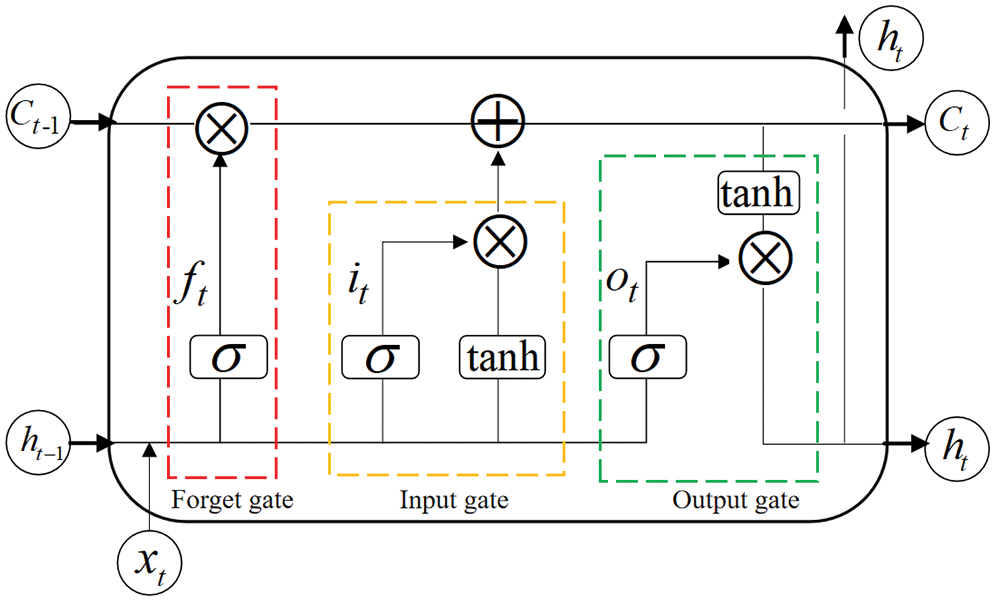
Figure 1: LSTM neuron internal structure

The forget gate is composed of the activation function σ, and its state update calculation formula is shown in Eq. (2). It decides if the memory unit ct−1 should be retained or thrown away.

ft=σ(Wf⋅[ht−1,xt]+bf)(2)

The input gate consists of activation functions σ and tanh, which is updated by Eq. (3), whose role is to regulate the degree to which the information c~t obtained by Eq. (4) is preserved to ct. The update of ct is completed by Eq. (5)

it=σ(Wi⋅[ht−1,xt]+bi)(3)

c~t=tanh⁡(Wc⋅[ht−1,xt]+bc)(4)

ct=ft⊗ct−1+it⊗c~t(5)

The output gate is composed of the activation functions σ and tanh, whose update equation is (6), and finally, the update of ht is completed by Eq. (7).

ot=σ(Wo⋅[ht−1,xt]+bo)(6)

ht=ot⊗tanh⁡(ct)(7)

In the above equations, W and b denote the weights and biases, respectively, and ⊗ denotes the product operation.

3  Design of HF-UHF RFID Tag Antenna

3.1 HF-UHF RFID Chip

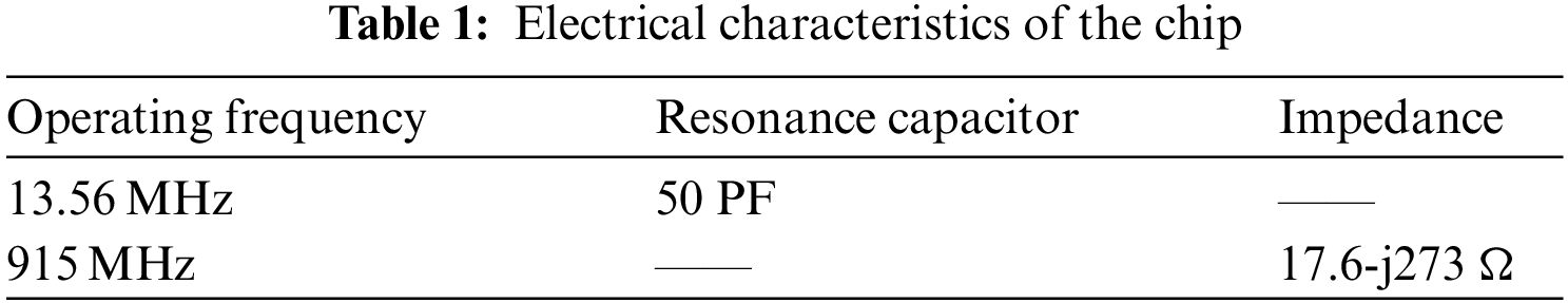
The RFID tag chip in this paper is em|echo-V produced by EM Microelectronics, which is a dual frequency device that supports ISO/IEC15693, ISO/IEC18000-3 model 1, NFC Forum Type 5 Tag, ISO/IEC18000-63, EPCTM Gen2v2, and ISO/IEC29167-10. The electrical characteristics of the chip are shown in Table 1 [20].

3.2 Design Goal of the HF-UHF RFID Tag Antenna

The energy source of the passive RFID tags is only the radio frequency energy transmitted by the RFID readers in the air. To improve the response distance of the tag, the antenna of the tag should have a good impedance match with the chip used, according to the maximum power transmission theory. The return loss (S11) of the tag antenna port can effectively measure the degree of impedance matching between the antenna and chip. The S11 is computed by

S11=20lg⁡(Za−Zc∗Za+Zc)(8)

where Za is the antenna input impedance, Zc is the chip input impedance and Zc∗ is the conjugate value of chip impedance. According to the engineering requirements, this paper takes S11≤−10 dB as the design goal of the HF-UHF RFID tag antenna.

3.3 Structure of the HF-UHF RFID Tag Antenna

The simulation software used in this research is Ansoft High Frequency Structure Simulator (HFSS) 19.2; the computer hardware configurations are Intel (R) Core (TM) i7-9750HF CPU @ 2.60 GHz and 32G RAM.

The designed RFID tag antenna comprises a HF coil antenna and an UHF folded dipole antenna. Fig. 2 shows the structure of the HF coil antenna. The coil antenna distributes on both sides of the substrate in the form of a via-hole connection, and the winding direction is counterclockwise. The turn width and turn spacing of the coil antenna are represented by m and s. As shown in Fig. 3, the UHF antenna is a left-right symmetrical folded dipole antenna with a matching ring, and the end of the antenna are radiation patches; the overall structure of the HF-UHF RFID tag antenna is demonstrated in Fig. 3. The antenna builds on a polyethylene terephthalate film substrate of 2.7 relative permittivity and 0.075 mm of thickness, whose size varies with the dout in the HF RFID tag antenna and the a2 in the UHF RFID tag antenna.

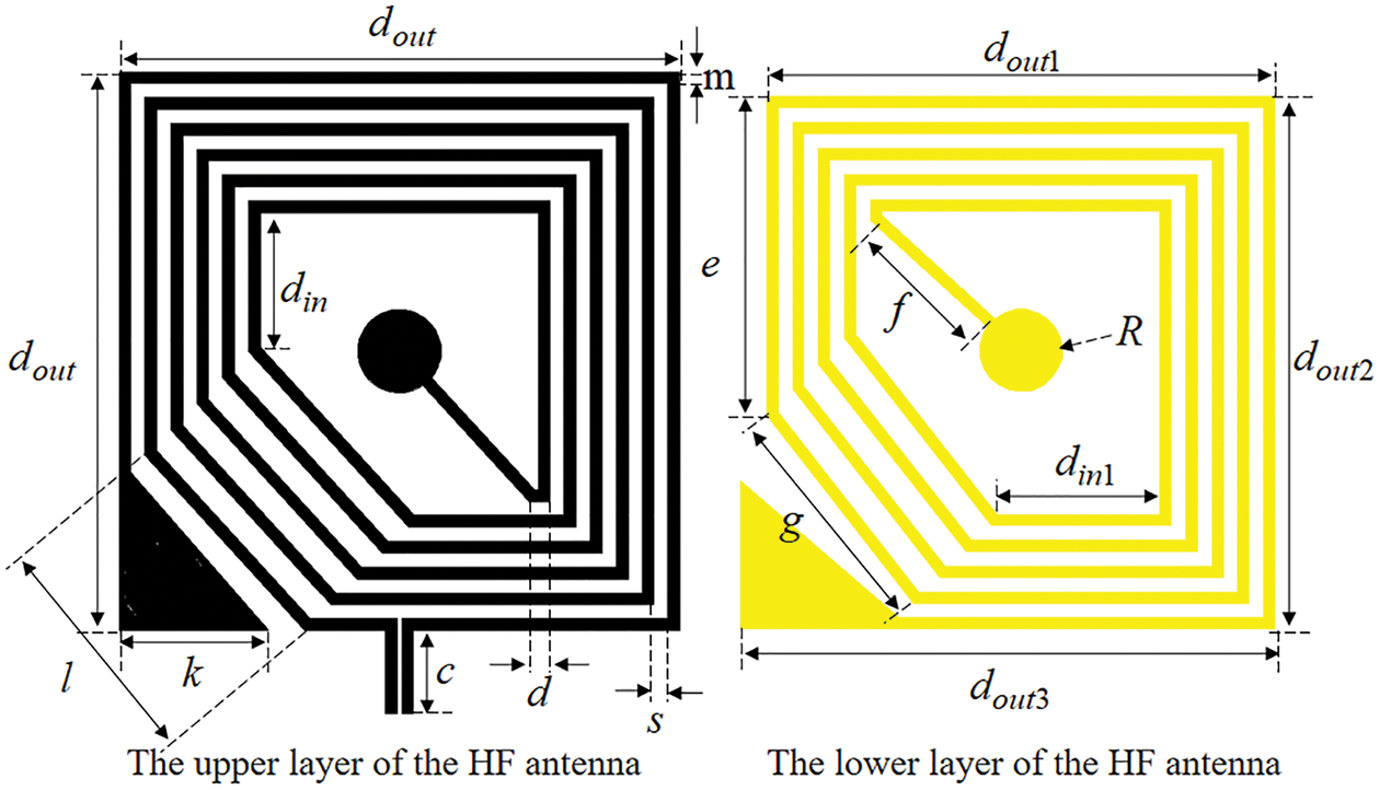
Figure 2: Structure of the HF RFID tag antenna

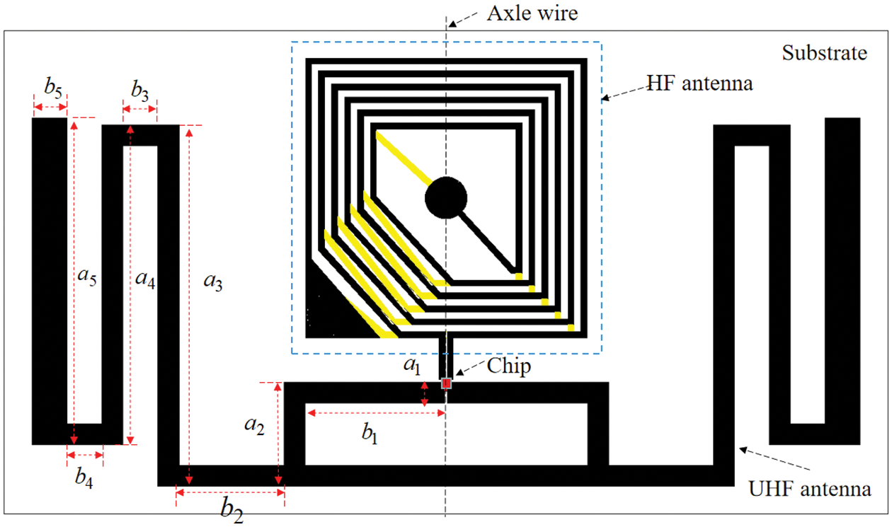
Figure 3: Structure of the HF-UHF tag antenna

Through experiments, it is found that the average simulation time of the HF RFID tag antenna is about 16 s, which is only 1/3 of the UHF antenna. This is because the mesh size of the finite element analysis method profile is related to the wavelength of the antenna, and the wavelength of the HF antenna is much larger than that of the UHF antenna. As a result, the HF antenna is relatively computationally small and the simulation time is comparatively short. As explained in [21], the HF RFID tag antenna has a significant impact on the impedance of the UHF RFID tag antenna, while the latter has a relatively small influence on the former. Therefore, this paper will obtain the structural dimensions of the HF coil antenna with the help of HFSS simulation software and design the UHF antenna based on it. Table 2 shows the dimensions of the HF antenna obtained from the simulation experiment. To prevent the UHF antenna from contacting the HF antenna, overlapping itself, or exceeding the substrate, its dimensions must meet the following formulas:

{b1+b2>dout/2a2>2a1a3<a2+c+douta4<a3a5≈a4(9)

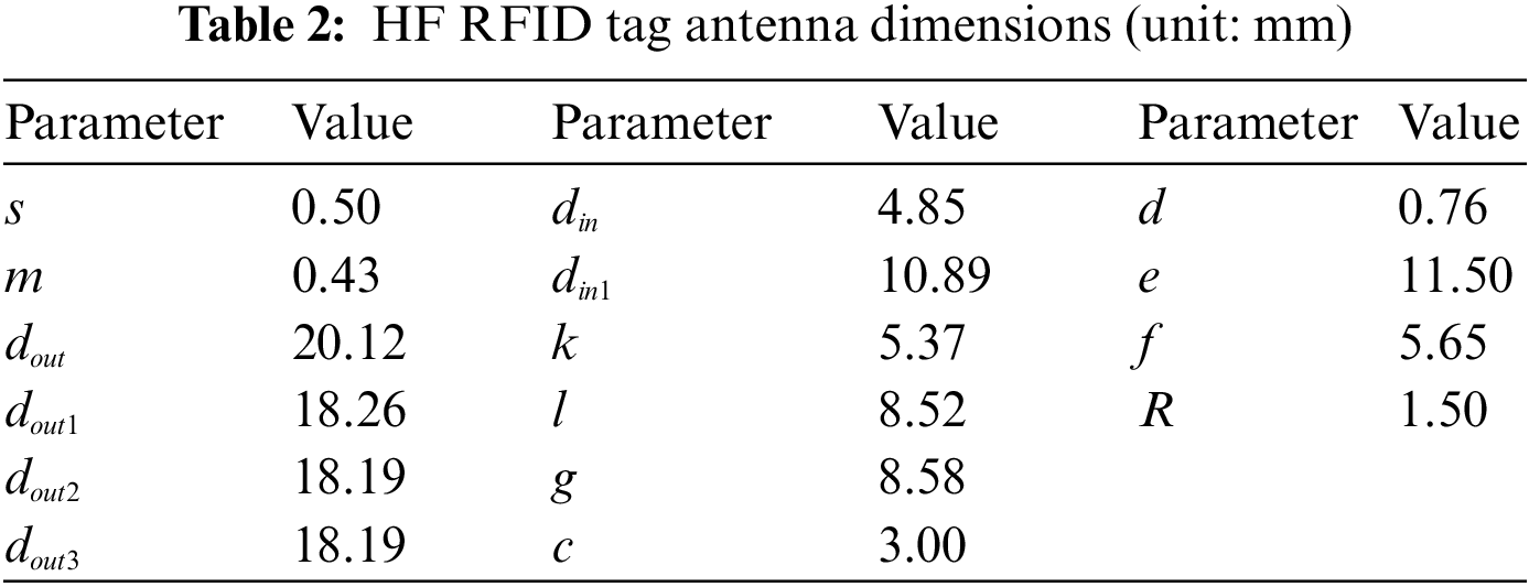
Table 3 shows the range of the structure parameters of the UHF antenna.

4  MSCNN-LSTM Model Experiment

4.1 Data Preparation

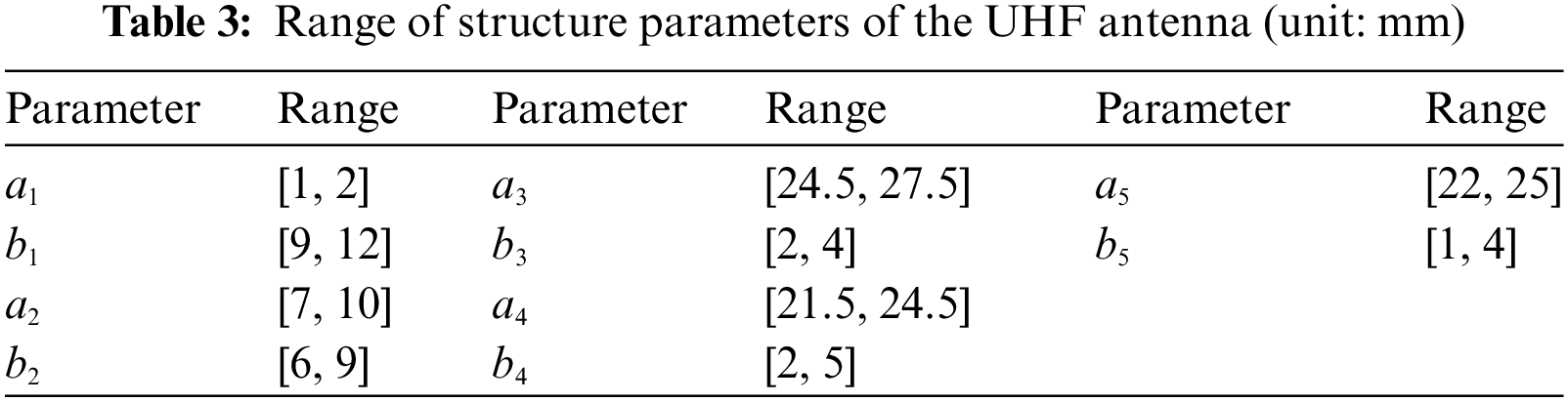
Based on the initial structure of the HF-UHF RFID tag antenna shown in Fig. 3, this study used MATLAB to control the HFSS to randomly adjust the dimensions of the UHF antenna according to Table 3 to generate a total of 480 sets of antenna simulation data. Then, in the working frequency band (860 –960 MHz) of the UHF RFID tag antenna with a sampling interval of 4 MHz, the return loss of antennas at 21 frequency points were taken respectively, and 480 groups of antennas collected a total of 10,080 sample data.

4.2 Data Analysis

This section firstly introduces the structure of the UHF antenna, then shows the impact of each dimension change on UHF antenna impedance and explains the reason for changes from the principle, and finally infers the characteristics of UHF antenna dimension data and the relationship between the dimension and antenna return loss.

As shown in Fig. 4, the UHF antenna is a left-right symmetric structure with an impedance matching ring in the middle, a folded dipole connected to the matching ring, and radiating patches [22] at the end. a1 represents the line width of the matching ring and the folded dipole, b5 represents the width of the radiation patches. The dimensions of the structures to the left from the center axis of the UHF antenna are b1, a2, b2, a3, b3, a4, b4 and a5, respectively.

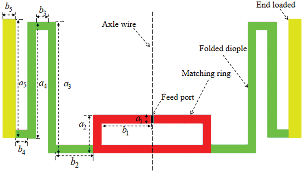
Figure 4: Structural division diagram of the UHF antenna

Fig. 5 presents the simulation result of UHF RFID tag antenna impedance changing with each dimension adjustment. The results show that the antenna impedance is related to each dimension, but there are differences in the degree of correlation. For example, b1 and a3 are increased by 3 mm in steps of 0.5 mm the former increases the antenna reactance and resistance by about 108 and 28 Ω, respectively; the latter can only change it by 17 and 4 Ω. The effect of the same dimension alteration on the resistance and reactance of the antenna is generally the same. Still, there are exceptions, and the b4 is a case in point, when b4 increases from 4 to 4.5 mm, the resistance of the antenna increases, and the reactance decreases. Finally, combined with Fig. 4, one can observe that the dimensions of the matching ring and the end radiation patches have a significant influence on the impedance of the UHF RFID tag antenna. This is because the ring structure can introduce inductance and capacitance, and the end-loading method can accumulate more charges and increase the equivalent capacitance of the tag antenna [22].

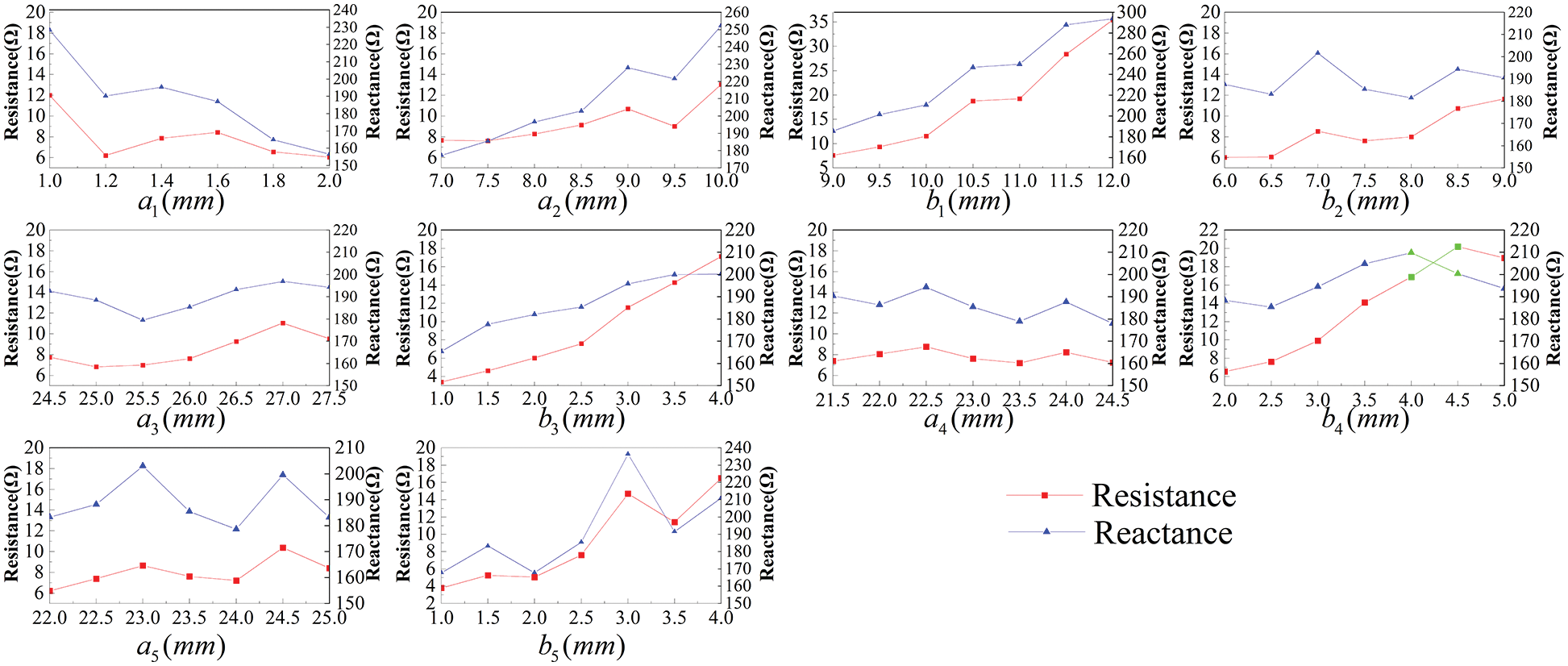
Figure 5: Simulation results of the UHF RFID tag antenna impedance variation with each dimension

To sum up, we draw the following conclusions: the data of dimensions not only represents the dimensions of different structures of the antenna, reflecting the spatial features of the antenna but also implies the impedance characteristics of different structures, which determine the overall impedance of the antenna to a large extent.

As shown in Fig. 6, the return loss of the UHF RFID tag antenna varies with the antenna dimensions. According to the formula (8), UHF antenna return loss is related to the impedance of both the antenna and the chip, and the impedance of the chip at a specific frequency has been relatively fixed. Hence, it depends on the impedance of the antenna. Due to the impedance of the antenna is not linearly related to the dimensions, the return loss of the antenna is also a nonlinear mapping relationship with the dimensions.

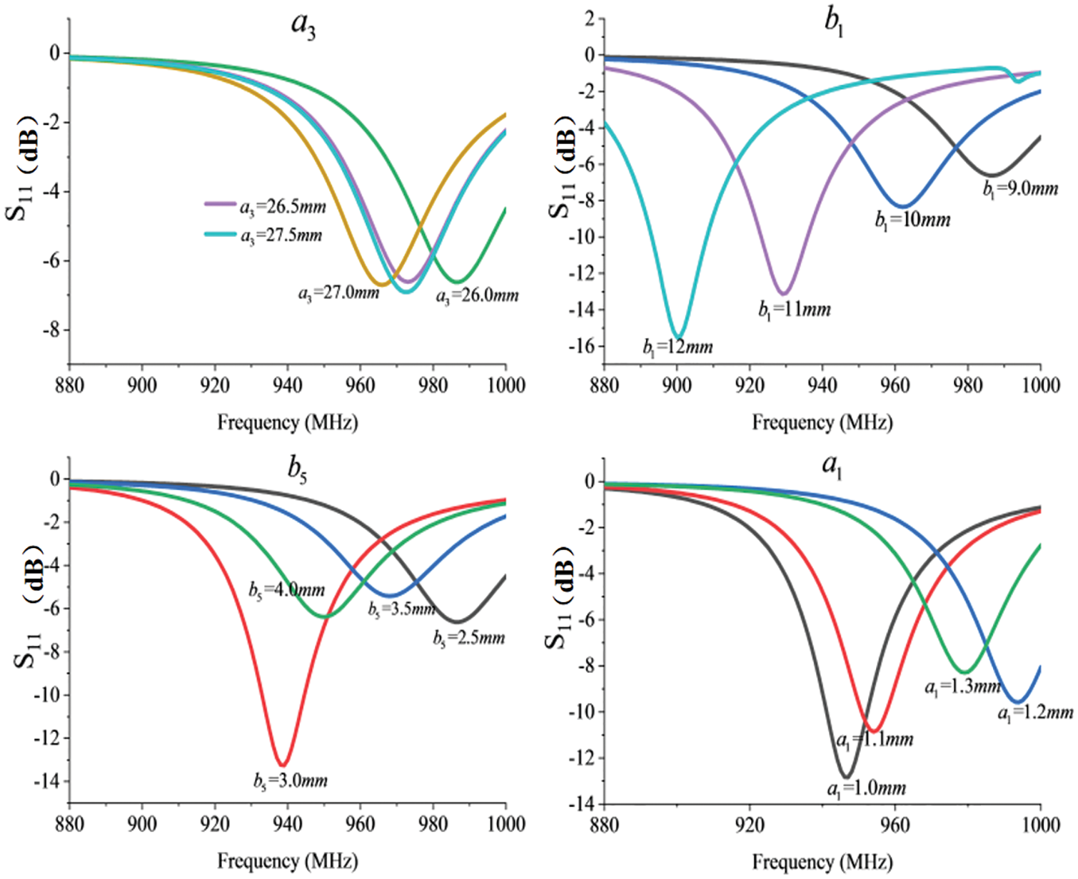
Figure 6: Simulation results of UHF RFID tag antenna return loss variation with each dimension

4.3 MSCNN-LSTM Model

In this section, to obtain the non-linear mapping relationship between UHF antenna return loss and its dimensions, the MSCNN-LSTM model is established based on the spatial features of the antenna simulation data and the impedance characteristics implied by it. The model of the MSCNN-LSTM is shown in the inset of Fig. 7.

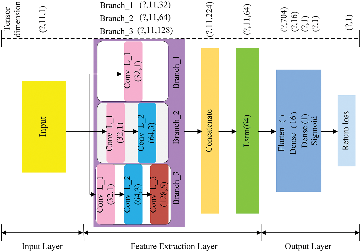
Figure 7: Structure of the MSCNN-LSTM

In the MSCNN-LSTM, ten structural parameters (a1,b1,a2,b2,a3,b3,a4,b4,a5,b5) of the UHF antenna and one sampling frequency point are set as input, and the return loss of the antenna is set as output. The input shape is (?, 11, 1), “?” indicates the number of samples delivered per batch of training, which is taken as 10 in this article. 11 and 1 represent the length and dimension of the input, respectively. The feature extraction layer is divided into the MSCNN module, Concatenate module, and LSTM module. MSCNN has three branches, Branch_1 has one dimensional convolution layer_1 (Conv L_1), Branch_2 contains Conv L_1 and Conv L_2, and Branch_ 3 consists of three convolution layers, Conv L_1, Conv L_2, Conv L_3 in that order. The parameters of Conv L_1, Conv L_2 and Conv L_3 are (32, 1), (64, 3) and (128, 5), respectively. Where 32, 64, 128 represent the number of convolution kernels, and 1, 3, and 5 are the size of the kernels. Conv L_1 uses relatively small convolution kernels, which can automatically extract fine-grain features of the antenna. Conv L_2 has a medium-sized kernel to extract the relatively coarse grain features of the antenna. Whereas, Conv L_3 extracts the overall features of the antenna, hence uses the larger kernel [15]. In addition, as the convolution depth increases and the size of the convolution kernels grows, more feature information is accumulated, and we increase the number of convolution kernels in the later convolution layers to fully extract the feature information. In each convolutional layer, the stride is 1, the padding is SAME, and the activation function is rectified linear unit (ReLU) which can improve the training speed of neural networks. Passing through Branch_1, the tensor dimension of the input data becomes (?, 11, 32). In Branch_2, the input data passes through Conv L_1and then Conv L_2, and the dimension of the tensor becomes (? 11, 64). The input data passes through the three convolutional layers in Branch_3 in turn, and the tensor dimension is changed to (? 11, 128).

The Concatenate module connects the features from the three branches to obtain broader feature information. The output shape of Concatenate module is (?, 11, 224).

Long-term memory retention is one of the main advantages of LSTM. As demonstrated in [12], the LSTM also performs well in the prediction of antenna performance. This paper input the dimension data into the model in the order of the structure of the UHF RFID tag antenna so that the LSTM with 64 units can fully extract the EM characteristics of the antenna, after which the feature information is flattened into a vector of 704 by the flatten layer. The feature information then enters a fully connected layer consisting of two dense layers. Two dense layers can improve the accuracy of the prediction results. Finally, the last feature information is used to predict the return loss of the UHF antenna via the Sigmoid layer.

4.4 Training of MSCNN-LSTM Model

This paper built related algorithm models based on the deep learning framework TensorFlow.

At the beginning of model training, we normalized the sample data to [0, 1] to improve the efficiency of model training [23]. These 10080 samples were then randomly divided into training and testing sets in an 8:2 ratio. The parameters of the model were optimized using the Adam optimizer during the model training process, with the initial learning rate set to 0.001 and the number of iterations trained to 100. The top part of Fig. 7 shows the change in tensor dimension after the data has gone through each module.

4.5 Performance Analysis of MSCNN-LSTM

Four models of CNN, LSTM, CNN-LSTM and BiLSTM [9] with the same training parameters as the MSCNN-LSTM were built to verify the prediction ability of the MSCNN-LSTM model on the return loss of UHF antenna in HF-UHF RFID tag antenna. The prediction performance of each model was quantified by using the mean absolute error (MAE), mean square error (MSE), and root mean square error (RMSE) evaluation metrics. The evaluation metric is calculated as follows:

MAE=1n∑i=1n|yprei−ytruei|(10)

MSE=1n∑i=1n(yprei−ytruei)2(11)

RMSE=1n∑i=1n(yprei−ytruei)2(12)

Table 4 shows the prediction errors of MSCNN-LSTM, CNN-LSTM, LSTM, CNN, and BiLSTM [9] models in the test set and the time consumption comparison with HFSS for calculating the return loss of 100 UHF antennas. The smaller the value of each evaluation index of the model, the closer the predicted value of return loss is to the simulated value of HFSS, and the superior prediction performance of the model. As shown in Table 4, the MAE, MSE, and RMSE of MSCNN-LSTM are 0.0073, 0.00032, and 0.01814 are smaller than the evaluation results of other models, indicating that the MSCNN-LSTM model proposed in this paper is superior to CNN-LSTM, LSTM, CNN, and BiLSTM [9] in UHF antenna return loss prediction. The evaluation indexes of MSCNN-LSTM are better than those of CNN-LSTM, reflecting the comprehensiveness and superiority of MSCNN in extracting antenna spatial features. The error of CNN-LSTM is smaller than that of LSTM and CNN, which means that combining CNN and LSTM can make up for the shortcomings of each and give full play to the advantages of both to improve the accuracy for predicting antenna performance. It can also be found that the prediction accuracy of LSTM is slightly higher than that of CNN, which is related to the electromagnetic characteristics of the different structures of the antenna, and it is difficult to reflect this intrinsic difference from the shape of the antenna alone. Table 4 shows that the BiLSTM [9] is marginally more precise than the LSTM, but it is not as powerful as the combination of the LSTM and CNN.

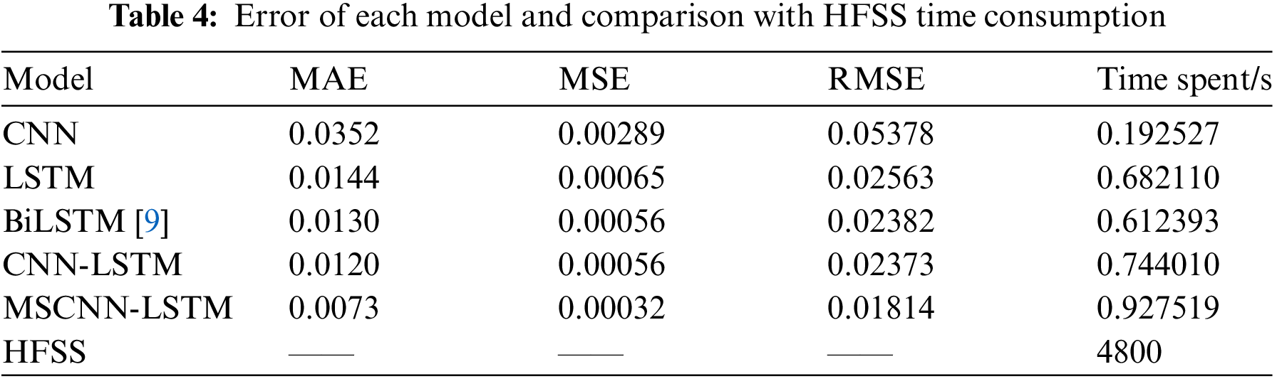
On the other hand, from the perspective of computation time, MSCNN-LSTM and other comparative models can evaluate the return loss of 100 UHF antennas in less than 1 s, while HFSS requires 4800 s. MSCNN-LSTM is relatively complex in terms of network structure, causing it to fall behind in terms of time consumption. Still the difference of less than 1 s between the models is entirely negligible compared to the simulation time of HFSS.

Fig. 8 shows the prediction performance of the MSCNN-LSTM model in partial test sets, the black dash-dot line represents the simulated values of the return loss of different antennas at different frequencies, and the red dash-dot line indicates the predicted values. In Fig. 8, the black simulation value distribution is irregular. However, each red prediction value is still very close to the black simulation value, which proves that the model can effectively predict the return loss of the UHF antenna.

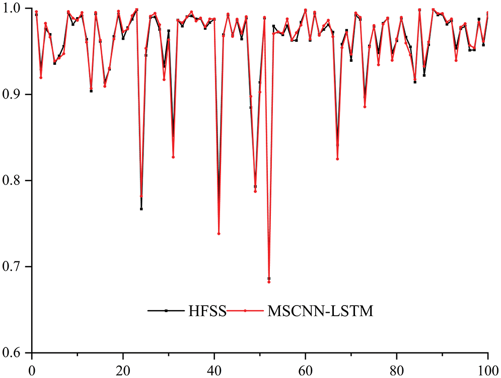
Figure 8: Example of MSCNN predictions

The prediction results of each model for some UHF antennas that are not in the sample data demonstrated in Fig. 9, from which it can be found that the predicted values of MSCNN-LSTM are closer to the simulation value of HFSS, and the prediction performances surpass that of CNN-LSTM and LSTM. Moreover, the accuracy of the MSCNN-LSTM in predicting the return loss near the resonance point is also improved compared to the literature [24], which is invaluable as the return loss at the impedance matching point of the RFID tag antenna usually drops dramatically, making it more difficult to predict.

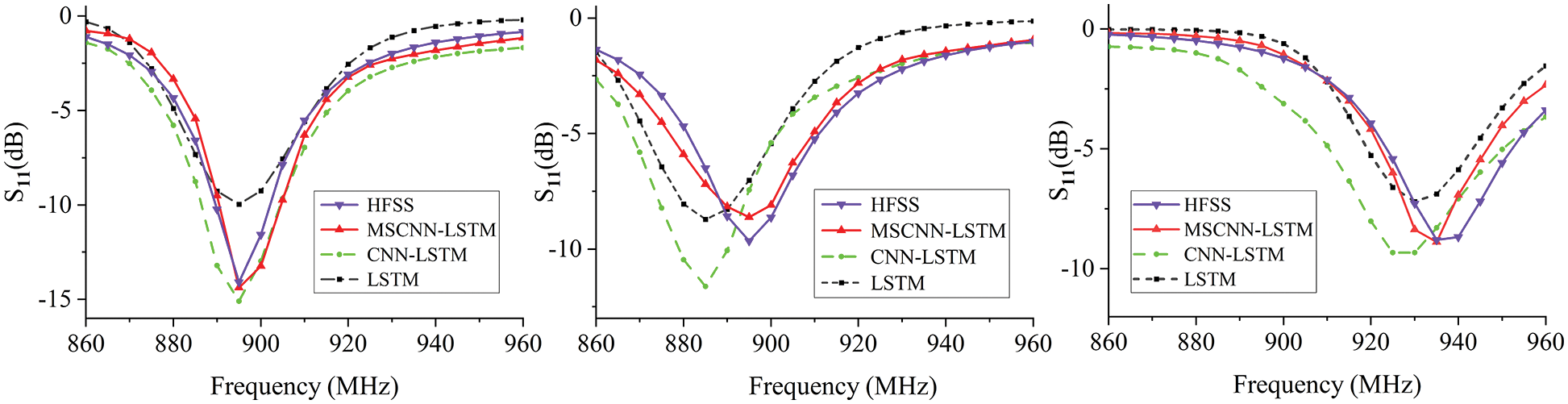
Figure 9: Prediction effect of each model for UHF antennas

Combining Table 4, Figs. 8 and 9, it can be concluded that compared to HFSS simulation calculation, MSCNN-LSTM greatly reduces the computational time consumption with guaranteed prediction accuracy, providing a basis for the fast design of HF-UHF RFID tag antennas.

4.6 Determine the Antenna Dimensions of the HF–UHF RFID Tag

Table 5 shows a set of UHF antenna dimensions with good return loss at 915 MHz predicted using the MSCNN-LSTM. Combined with the dimensions of the HF antenna in Section 3, the dimensions of the HF-UHF RFID tag antenna were determined in this paper.

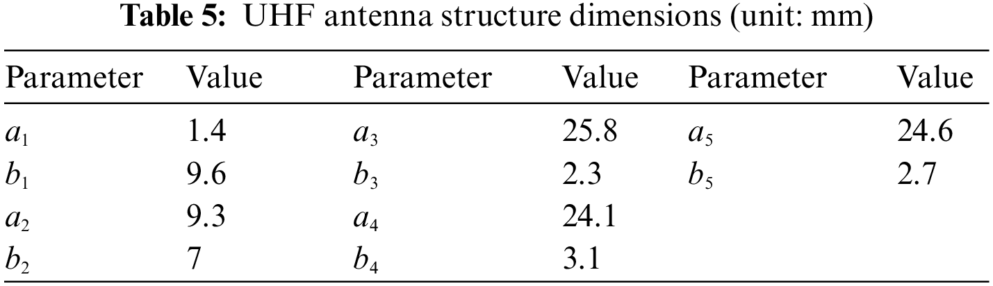
Fig. 10 depicts the return loss of the designed HF-UHF RFID tag antenna. In Fig. 10, the return loss of the HF antenna at 13.56 MHz is −58.76 dB, and the return loss of the UHF antenna at 915 MHz is −22.63 dB, both of which are less than −10 dB, indicating that the antenna and the chip have good impedance matching. The design goal of the HF UHF RFID tag antenna has been achieved.

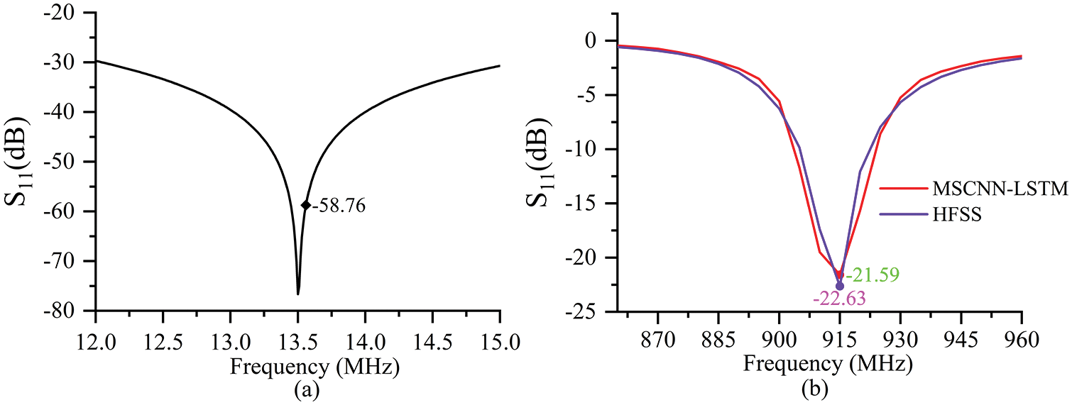
Figure 10: (a) Return loss of HF antenna; (b) Return loss of UHF antenna

5  Conclusion

In this paper, a new deep learning framework called MSCNN-LSTM has been proposed for predicting the return loss of the UHF antenna in HF-UHF RFID tag antenna, which is comprised of multi-scale convolutional neural network and long short-term memory. The model combines the advantages of both MSCNN and LSTM networks, which can extract fine-grain localized information of the antenna as well as overall spatial features and learn the EM characteristics of the different structures of the antenna. The proposed MSCNN-LSTM was validated using simulated data of UHF antennas in HF-UHF RFID antennas and compared with other prediction methods. Experimental results showed that the MAE (0.0073), MSE (0.00032), and RMSE (0.01814) of MSCNN-LSTM were the smallest compared to CNN, LSTM, BiLSTM, and CNN-LSTM. MSCNN-LSTM was significantly more accurate in predicting the return loss of UHF antennas than the previous four. In terms of computational time consumption, MSCNN-LSTM had a significant advantage over the simulation time of HFSS. The return loss of the dual-band RFID tag antenna designed with the assistance of MSCNN-LSTM was −58.76 and −22.63 dB at 13.56 and 915 MHz, respectively, which was a good conjugate match with the chip used and achieved the desired goal. In future research, we will try to refine the structure of the MSCNN-LSTM and apply it to the design of other antennas.

Acknowledgement: We sincerely thank our colleagues who contributed to the article but were not mentioned.

Funding Statement: The research work is carried out under the Beijing Natural Science Foundation-Beijing Education Commission Joint Project (KZ202210015020), Discipline Construction and Postgraduate Education Project of BIGC (No. 21090122005) and BIGC Project (Ee202204).

Conflicts of Interest: The authors declare that they have no conflicts of interest to report regarding the present study.

References

1. H. S. Farahani, B. Rezaee, M. Gadringer, W. Bosch, L. Zoscher et al., “A miniaturized HF/UHF dual-band RFID tag antenna,” in 2021 IEEE Int. Symp. on Antennas and Propagation and USNC-URSI Radio Science Meeting (APS/URSI), Singapore, pp. 383–384, 2021. [Google Scholar]

2. A. Sakonkanapong and C. Phongcharoenpanich, “Near-field HF-RFID and CMA-based circularly polarized far-field UHF-RFID integrated tag antenna,” International Journal of Antennas and Propagation, vol. 2020, pp. 1–15, 2020. [Google Scholar]

3. P. Wang, L. Dong, H. Wang, G. Li, Y. Di et al., “Passive wireless dual-tag UHF RFID sensor system for surface crack monitoring,” Sensors (Basel), vol. 21, no. 3, pp. 1–16, 2021. [Google Scholar]

4. N. Ha-Van and C. Seo, “A single-feeding port HF-UHF dual-band RFID tag antenna,” Journal of Electromagnetic Engineering and Science, vol. 17, no. 4, pp. 233–237, 2017. [Google Scholar]

5. A. I. Hammoodi, M. Milanova and H. Khaleel, “Design of flexible antenna for UWB wireless applications using ANN,” in 2017 Int. Conf. on Computational Science and Computational Intelligence (CSCI), USA, pp. 751–754, 2017. [Google Scholar]

6. A. Chandio, G. Gui, T. Kumar, I. Ullah, R. Ranjbarzadeh et al., “Precise single-stage detector,” arXiv preprint arXiv:2210.04252, pp. 1–33, 2022. [Google Scholar]

7. W. Khan, K. Raj, T. Kumar, A. M. Roy and B. Luo, “Introducing urdu digits dataset with demonstration of an efficient and robust noisy decoder-based pseudo example generator,” Symmetry, vol. 14, no. 10, pp. 1–15, 2022. [Google Scholar]

8. X. Li, J. Gao and G. Boeck, “Printed dipole antenna design using artificial neural network modeling for RFID application,” International Journal of RF and Microwave Computer-Aided Engineering, vol. 16, no. 6, pp. 607–611, 2006. [Google Scholar]

9. T. Hong, Z. He, C. Wang, J. Chen and J. Zhou, “Fast multi-objective RFID tag antenna design based on BiLSTM surrogate model,” Journal of Microwaves, vol. 37, no. 1, pp. 21–27, 2021. [Google Scholar]

10. R. S. Daniel, “Multiband substrate integrated waveguide antenna loaded with slots using artificial neural network,” International Journal of RF and Microwave Computer-Aided Engineering, vol. 32, no. 10, pp. 1–12, 2022. [Google Scholar]

11. A. Katkevičius, D. Plonis, R. Damaševičius and R. Maskeliūnas, “Trends of microwave devices design based on artificial neural networks: A review,” Electronics, vol. 11, no. 15, pp. 1–21, 2022. [Google Scholar]

12. D. Sami Khafaga, A. Ali Alhussan, E. -S. M. El-kenawy, A. Ibrahim, S. H. Abd Elkhalik et al., “Improved prediction of metamaterial antenna bandwidth using adaptive optimization of LSTM,” Computers, Materials & Continua, vol. 73, no. 1, pp. 865–881, 2022. [Google Scholar]

13. J. P. Jacobs, “Accurate modeling by convolutional neural-network regression of resonant frequencies of dual-band pixelated microstrip antenna,” IEEE Antennas and Wireless Propagation Letters, vol. 20, no. 12, pp. 2417–2421, 2021. [Google Scholar]

14. H. -Y. Luo, Y. Hong, Y. -H. Lv and W. Shao, “Parametric modeling of UWB antennas using convolutional neural networks,” in 2020 IEEE Int. Symp. on Antennas and Propagation and North American Radio Science Meeting, Montreal, Quebec, Canada, pp. 2055–2056, 2020. [Google Scholar]

15. A. M. Roy, “Adaptive transfer learning-based multiscale feature fused deep convolutional neural network for EEG MI multiclassification in brain–computer interface,” Engineering Applications of Artificial Intelligence, vol. 116, pp. 1–17, 2022. [Google Scholar]

16. P. R. Kanna and P. Santhi, “Hybrid intrusion detection using mapreduce based black widow optimized convolutional long short-term memory neural networks,” Expert Systems with Applications, vol. 194, pp. 116545, 2022. [Google Scholar]

17. P. Rajesh Kanna and P. Santhi, “Unified deep learning approach for efficient intrusion detection system using integrated spatial–temporal features,” Knowledge-Based Systems, vol. 226, pp. 1–12, 2021. [Google Scholar]

18. Y. LeCun, L. Bottou, Y. Bengio and P. Haffner, “Gradient-based learning applied to document recognition,” Proceedings of the IEEE, vol. 86, no. 11, pp. 2278–2324, 1998. [Google Scholar]

19. A. S. Navathe, M. Mugiishi and E. J. Emanuel, “Population-based primary care payment system in Hawaii-reply,” JAMA, vol. 322, no. 21, pp. 2136–2137, 2019. [Google Scholar] [PubMed]

20. https://www.emmicroelectronic.com/product/nfc-high-frequency-ics/em-echo-v [Google Scholar]

21. Z. Yang, Y. Zhang, L. Zhu, L. Shen, Y. Du et al., “Design of a single chip HF-UHF dual-band RFID tag antenna,” in Interdisciplinary Research for Printing and Packaging, Springer, Singapore, pp. 301–305, 2022. [Google Scholar]

22. N. Faudzi, M. Ali, I. Ismail, H. Jumaat and N. Sukaimi, “A compact dipole UHF-RFID tag antenna,” in 2013 IEEE Int. RF and Microwave Conf. (RFM), CA, USA, pp. 314–317, 2013. [Google Scholar]

23. S. Ioffe and C. Szegedy, “Batch normalization: Accelerating deep network training by reducing internal covariate shift,” in Int. Conf. on Machine Learning, PMLR, pp. 448–456, 2015. [Google Scholar]

24. Y. -F. Liu, L. Peng and W. Shao, “An efficient knowledge-based artificial neural network for the design of circularly polarized 3-D-printed lens antenna,” IEEE Transactions on Antennas and Propagation, vol. 70, no. 7, pp. 5007–5014, 2022. [Google Scholar]