Identification of Rice Leaf Disease Using Improved ShuffleNet V2

1  Introduction

In China, rice plays an important role in grain production. However, rice disease affects the growth of rice, which is an obstacle to rice yield. At present, there are many kinds of rice diseases [1–3]. Traditional identification methods rely on manual treatment to subjectively identify a variety of rice diseases, which consumes a lot of manpower and time [4]. The traditional disease identification methods have not met the production requirements of modern agriculture. It is urgent to develop a fast and accurate rice disease identification system to guide farmers to use pesticides correctly, reduce economic losses caused by diseases, and improve rice yield.

Now, image processing and machine learning are the key technologies to realize the identification and detection of plant diseases and pests [5–8]. Xiao et al. [9] realized the identification of common vegetable pests using the word bag model and support vector machine (SVM), with an average identification rate of 91.56%. Shi et al. [10] proposed a kernel discrimination method based on the spectral vegetation index (SVIKDA) to detect winter wheat diseases. The experimental results showed that the classification accuracy of mild, moderate, and severe winter wheat diseases could reach 82.9%, 89.2%, and 87.9%, respectively. Zhu et al. [11] proposed an automatic detection method of grape leaf disease based on image analysis and a back propagation neural network (BPNN). They extracted characteristic parameters such as perimeter, area, roundness, rectangle, and shape complexity by segmenting grape leaf disease regions. Finally, the average identification rate of the BPNN method can reach 91%. Besides, Singh et al. [12] applied the SVM to identify healthy and diseased rice plants, with an accuracy of 82%. Although image processing and machine learning technology have promoted the development of plant disease identification and detection technology, these methods not only require manual participation, but also need to know a lot of professional knowledge to complete [13,14]. Especially in the natural environment, due to the poor ability of feature extraction, the identification accuracy of these methods will further decrease. Therefore, how to solve the problem of low efficiency of machine learning data processing, feature extraction and identification is an urgent work to promote the application of plant disease identification technology in practice.

With the development of deep learning, it has been widely used in image identification technology [15–17]. Convolutional neural network (CNN) in deep learning has developed into one of the best classification methods in image identification tasks. Different from machine learning, CNN has more powerful image feature learning and expression capabilities. CNN can automatically extract low-level features of images and further learn high-level features [18,19]. In addition, CNN can also learn the inherent rules of image samples to obtain the hidden feature information in the image. Therefore, CNN has been widely used in image identification, classification, and segmentation instead of machine learning [20–23]. Chen et al. [24] used deep transfer learning for image-based plant disease identification. The results demonstrated the average identification accuracy can reach 92% under complex background conditions. Rahman et al. [25] fine-tuned the advanced large-scale architecture (VGG16 and Inception V3) and used it to identify rice diseases and pests. The final identification accuracy can reach 93.3%. Wu et al. [26] adjusted the parameters of VGG16 and ResNet dual channel convolution neural network, and the identification accuracy of maize leaf disease can reach 93.33%. Suo et al. [27] developed a new network with CoAtNet as the backbone network to realize the identification of grape leaf diseases, with an identification accuracy of 95.95%. Lv et al. [28] designed a new neural network based on the backbone AlexNet architecture to identify maize diseases, with an accuracy of 98.62%. Zeng et al. [29] proposed a SKPSNet-50 convolution neural network model for maize disease identification. In natural scenes, the average identification accuracy of the model can reach 92.9%. Although deep learning has promoted the development of plant disease identification technology, the problems of excessive parameters, large model size, and low identification accuracy still need to be further solved.

Therefore, we proposed an improved ShuffleNet V2 in the research of rice disease identification based on Ghost Module and ECA. The improved ShuffleNet can name it GE-ShuffleNet. Firstly, to train and verify the model, rice disease images are enhanced to expand the image data set and diversify the complexity of the image background. Secondly, the Ghost Module is used to replace the 1 × 1 convolution of the two basic unit modules in ShuffleNet V2. The ReLU activation function is replaced by the Hardswish activation function to improve the identification accuracy of the model. In addition, the ECA module and L2 regularization are respectively used to extract the correlation between channels and prevent overfitting. Finally, the enhanced image is input into the improved model for training and verification. A large number of experimental results show that the proposed model is feasible and has more advantages (accuracy and model size) in comparison to other models. As shown in Fig. 1, it is the process of rice disease identification based on GE-ShuffleNet.

Figure 1: The schematic diagram of rice disease identification based on GE-ShuffleNet. The red and purple dotted line boxes are the process of data preprocessing and data set division; The blue dotted box is the process of model construction and parameter optimization; The identification result output of the model and the model comparison process are shown in the black dotted box at the bottom of the schematic diagram

2  Image Data Set and Preprocessing

2.1 Original Data Set

In our work, the rice leaf disease data set used for the model experiment is derived from the public data set of Rice Leaf Disease Image Samples [30], including four rice leaf diseases (Bacterial blight, Blast, Tungro, and Brown spot). To ensure the robustness of the designed model in the natural environment, we only selected 1068 images with complex backgrounds, including 293 Bacterial blight images, 269 Blast images, 245 Tungro images, and 261 Brown spot images. As shown in Figs. 2, 2a–2d are sample images of four rice diseases.

Figure 2: The sample images of four rice diseases. (a) Bacterial blight image; (b) Blast image; (c) Tungro image; (d) Brown spot image

2.2 Image Preprocessing

To ensure the diversity of the data set, these images are enhanced to make their backgrounds more complex. The selected rice disease images are enhanced by adding random pixels, Gaussian noise, salt and pepper noise, random occlusion, animation effects, random contrast, and Gaussian blur, respectively. In addition, the brightness and blurriness of these images are adjusted to simulate the natural environment. The total number of enhanced rice disease images was 5163, including 1416, 1311, 1303, and 1133 for Bacterial blight, Blast, Tungro, and Brown spot, respectively. The specific image information is described in Table 1. Besides, the enhanced images of four diseases are shown in Fig. 3.

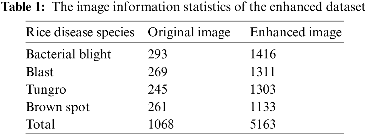
Figure 3: The enhanced sample images of four rice diseases. (a) Enhanced Bacterial blight image; (b) Enhanced Blast image; (c) Enhanced Tungro image; (d) Enhanced Brown spot image

To facilitate model training and testing, we divided the 5163 images, and selected about 80% of them (4132) as the training set, and the remaining 20% (1031) as the test set.

3  The Proposed GE-ShuffleNet

3.1 GE-ShuffleNet Model

In general, 1×1 Conv is used for two purposes before or after DWConv. On the one hand, it fuses information between channels to make up for the lack of information fusion function of DWConv between channels. On the other hand, it is used to reduce or increase dimensions, such as the inverted residual module in MobileNet V2. However, two 1×1 Conv are used in the right branch of shufflenet V2. In fact, only one is needed. Because 1×1 Conv is not required to play the role of dimension increase and dimension reduction, it is only used to fuse the information between channels of DWConv. First, the 1×1 Conv after DWConv in the right branch of ShuffleNet V2 is deleted. Secondly, to solve the problem that the remaining 1×1 Conv in ShuffleNet V2 occupies too much memory and causes the problem of computing load (FLOPs), the 1×1 Conv is replaced by the lightweight module Ghost Module in the GhostNet network [31]. In addition, ECA is added after the Ghost Module to effectively capture cross-channel interaction information under keeping the network lightweight. Finally, to avoid the overfitting problem of the model, L2 regularization is added to the network training. The ReLU activation function is replaced by the Hardswish activation function to further improve the identification accuracy of the model. The proposed structure diagram of GE-ShuffleNet is shown in Fig. 4.

Figure 4: The structure diagram of GE-ShuffleNet. Conv1 and Conv5 are convolution 1 and 5, respectively; MaxPool is the maximum pool layer; Stage2, stage3, and stage4 correspond to two basic units in part (a); Hardswish is the activation function; GlobalPool is global pooling; FC represents the full connection layer

3.2 ShuffleNet V2 Model

In addition to improving the accuracy of visual tasks, reducing the computational complexity of network models is also an urgent problem to be solved. Especially the hardware environment of the target platform is limited, so how to quickly identify the object with a very low delay. Due to the current actual demand, the network is developing towards lightweight, and they maintain a good balance between the running speed and accuracy of the model.

Ma et al. proposed ShuffleNet V2 based on ShuffleNet V1, and summarized four guidelines for designing efficient and lightweight networks [32–34]. As follows:

(1)   The input and output of the convolution layer keep the same number of channels, which can minimize the memory access cost (Memory Access Cost (MAC));

(2)   Consider the cost of using group convolution (excessive group convolution will increase MAC);

(3)   Reduce the number of branches and included units (the fewer branches in the model, the faster the model);

(4)   Reduce component-level operations (reduce time consumption).

As shown in Figs. 5, 5a and 5b are the basic units of ShuffleNet V1. However, the group convolution (GConv) and add operations in the red dashed boxes violate guidelines (2) and (4), respectively. In addition, the operations in the green box and the blue box in Fig. 5 violate guidelines (1) and (3), respectively. Therefore, to achieve high model capacity and efficiency, the key to solving the problem is to maintain a large number of channels with the same width, neither dense convolution nor multiple packets. As shown in Fig. 6, it is the schematic diagram of the ShuffleNet V2 basic unit module [35]. Observing Figs. 5 and 6, we can find that, different from ShuffleNet V1, ShuffleNet V2 (Fig. 6a) first splits the channel of the input characteristic matrix into two branches through a channel split. Here, the left branch is a shortcut branch, and the right branch corresponds to the main branch, thus meeting the guideline (3).

Figure 5: The basic unit of ShuffleNet V1. Input is the characteristic diagram input; GConv represents group convolution; DWConv represents depthwise convolution; AVGPool represents the average pooling layer; Stride is the step size; Concat indicates splicing operation; Add indicates element level addition operation; Output represents the output of the feature map; BN is batch normalization; ReLU is the activation function

Figure 6: The basic unit of ShuffleNet V2

The three convolutions input and output channels in the right branch have the same number, and the left and right branches are concatenated through the Concat module. In this way, the input and output of the convolution layer can maintain the same number of channels to reduce MAC (meeting the guideline (1)). We can also find that ShuffleNet V2 uses 1×1 convolution to replace the two GConvs in ShuffleNet V1. Since the use of group convolution is reduced, the MAC is also decreased. To increase information flow and realize feature mixing, in ShuffleNet V2, the channel Shuffle is connected after the Concat. Different from ShuffleNet V1, ReLU is placed on the right branch of ShuffleNet V2, which will reduce the number of processing elements by half. Besides, the ShuffleNet V2 uses a 3×3 depthwise convolution (DWConv) and a 1×1 convolution (Conv) instead of 3×3 average pooling (AVGPool) for feature mixing.

3.3 Ghost Module

Ghost Module is a model compression method. Compared with traditional convolution, Ghost Module can improve network speed by reducing network parameters and computation under ensuring network accuracy.

As the conventional convolution and Ghost Module are shown in Fig. 7. Observing Figs. 7a and 7b, we can find that the Ghost Module is divided into three steps to obtain the same number of feature maps as the conventional convolutions. Firstly, a small number of intrinsic feature maps are generated through traditional 1×1 convolution. Secondly, linear operations are used to expand features and increase the number of channels. These linear operations can generate more feature maps with fewer parameters. Without changing the size of the output feature map, the total number of parameters required in the Ghost Module and the computational complexity are lower than those of conventional CNN [36]. Finally, the output feature map after two convolutions is superimposed on the channel dimension to obtain the same output as the traditional convolution. Besides, Ghost Module can realize parallel identification and linear change, and reduce the computing cost of the general convolution layer while maintaining approximate identification performance.

Figure 7: The conventional convolution and Ghost Module. (a) Conventional convolution; (b) Ghost module. Identity refers to identity transformation; Φn represents a linear operation

3.4 ECA Attention Mechanism

The attention mechanisms can focus on important information with high weight. It can not only ignore irrelevant information with low weight, but also constantly adjust the weight to adapt to the selection of important information in different conditions. However, the current attention mechanism focuses more on the performance of selecting information that is more critical to the current task goal from a large amount of information, without considering the complexity of the model. The performance of the model is improved, but the complexity has also increased. To solve the contradiction between performance and complexity, Wang et al. [37] proposed an ECA module. The advantage of the ECA module is that it not only involves fewer parameters, but also has obvious performance gain.

As the schematic diagram of ECA attention mechanism is described in the Fig. 8. First, the input H×W×C feature map x is compressed by global average pooling (GAP) to obtain the 1×1×C feature map. Secondly, channel feature learning is carried out on the characteristic graph of 1×1×C, and local cross channel information interaction between each channel and adjacent K channels is realized by performing fast 1D convolution with the number of K. It should be noted that the value of K is adaptively determined and proportional to the mapping of channel coefficient C. Then 1×1 Conv is used to learn the interaction information between different channels. At this time, the dimension of the output feature map is still 1×1×C. Finally, the feature map 1×1×C of channel attention and the original H×W×C input feature map x are multiplied channel by channel through the ⊗ operator to obtain x1. x1 is a feature map with channel attention.

Figure 8: The schematic diagram of the ECA attention mechanism. GAP represents global average pooling; refers to the generation of channel weights using the Sigmoid activation function; ⊗ represents the element-by-element product operator

3.5 Hardswish Activation Function

In our work, we use the Hardswish activation function to replace the ReLU activation function of Conv1 and Conv5 in ShuffleNet V2 (as shown in Fig. 4). The ReLU activation function is shown in Eq. (1). Based on Eq. (1), the relationship between ReLU input x and output f(x) is shown in Fig. 9a. ReLU has the advantage that when x>0, its derivative is always 1, so there is no problem of gradient disappearance. In addition, ReLU is very fast in calculating derivatives. It only needs to judge whether x>0 or x<0. The disadvantage of ReLU is that some neurons may never be activated, resulting in the corresponding parameters never being updated. Because when x≤0, the output is always 0. If the output of a neuron is less than or equal to 0, it cannot enter the calculation. This phenomenon is called neuronal necrosis.

Figure 9: Activation function

The Hardswish activation function is proposed in MobileNet V3 [38]. The Hardswish activation function is an improvement of the swish activation function. The swish activation function is shown in Eq. (2). Based on Eq. (2), the relationship between swish input x and output f(x) is shown in Fig. 9b. Although compared with the ReLU activation function, swish can improve the accuracy of the neural networks to a certain extent, the derivation is more complex and quantization speed is slower. Therefore, from the perspective of actual embedded mobile devices, it does not meet the requirements of practical deployment. Hardswish has the same accuracy as swish, and can solve the problem of ReLU activation function neuron necrosis. Hardswish not only has the advantages of good numerical stability and fast computing speed, but also can be implemented as a segmentation function to reduce the number of memory accesses.

Therefore, Hardswish has significant advantages in deploying on practical embedded mobile devices. Eq. (3) is the Hardswish activation function. Fig. 9c shows the relationship between input x and output f(x) of Hardswish.

fReLU(x)=max{0,x}={x,ifx>00,otherwise(1)

fswish(x)=x⋅σ(x)(2)

fHardswish(x)=x⋅ReLU6(x+3)6={0,x≤−3x,x≥3x⋅(x+3)6, otherwise(3)

4  Experimental Results and Analysis

4.1 Experimental Environment and Hyperparameters Setting

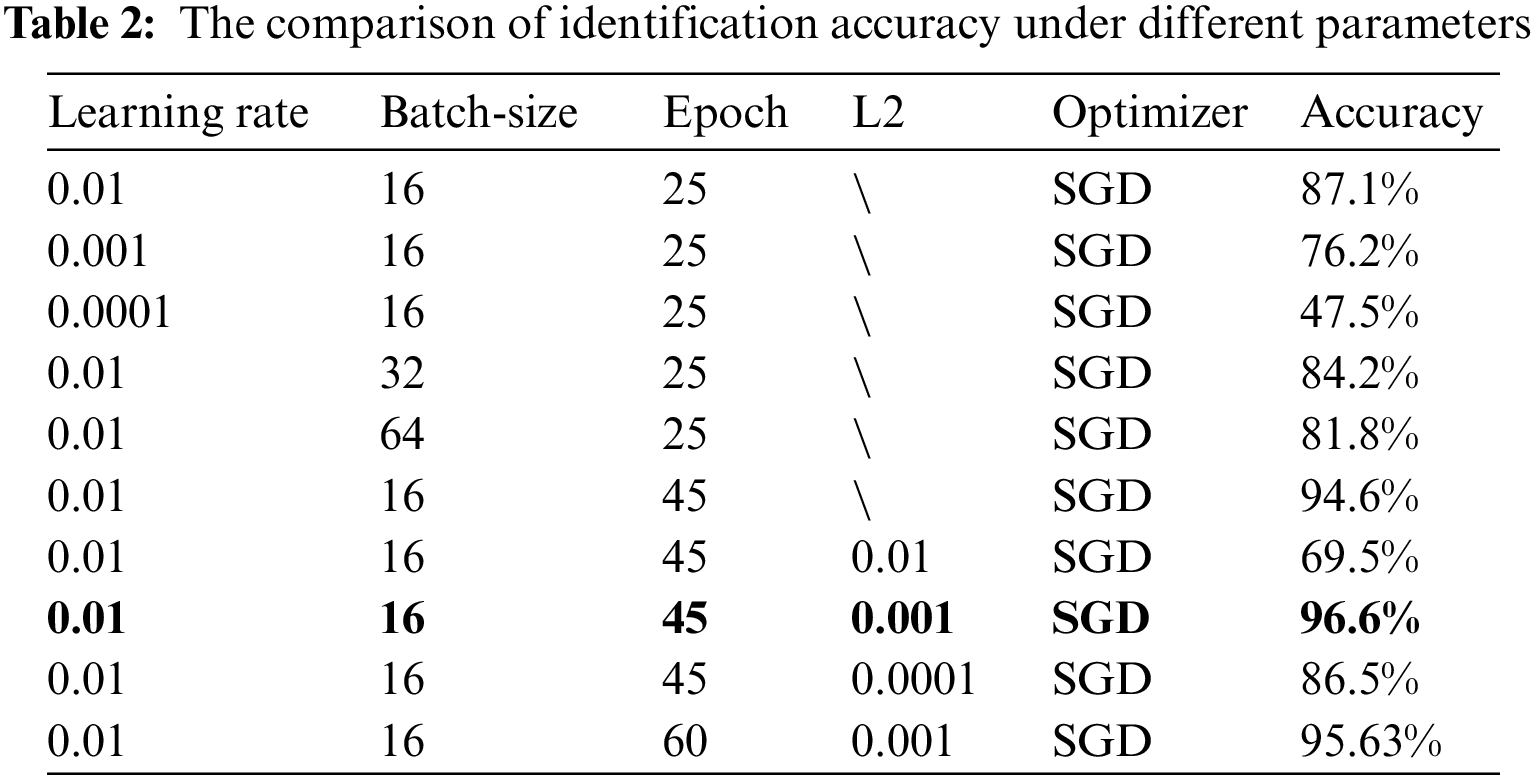
To implement our model training and validation, the experimental environment is python 3.8, PyTorch 1.9.1, and torch-vision 0.10.1. The server is configured with Intel Xeon E5-2680 v4 CPU, Samsung SSD 860 512 G hard disk, Kingston DDR4 64 GB memory, NVIDIA TITAN Xp graphics card, and 12 GB video memory. In the experiment, the stochastic gradient descent (SGD) optimizer is used to select the hyperparameters (learning rate, batch size, iterations, L2 regularization coefficient) of the model through a series of tests and comparative analysis. As shown in Table 2, the identification accuracy comparison of the GE-ShuffleNet model under the different parameters. Observing Table 2, we can find that the best highest accuracy (96.6%) can reach under learning rate (0.01), batch size (16), epoch (45), and L2 (0.001). Therefore, we set the learning rate, batch size, and L2 to 0.01, 16, and 0.001 to train our model under 45 epochs.

4.2 Analysis of Identification Results

The value stored in each element (i, j) represents the number of types (i) recognized by the classifier as type (j) when the actual category is type (i). Further, the model can calculate the identification accuracy and recall rate of each category. As shown in Figs. 10a and 10b correspond to the confusion matrix and normalized confusion matrix of the GE -ShuffleNet, respectively. From the normalized confusion matrix (Fig. 10b), we can see that the classification accuracy of our models for the four diseases is higher than 95%. In addition, we can see from the confusion matrix that the error rates of identification of Bacterial blight are 1.946%, 0.457%, and 0.755%, which are confused with Blast, Brown spot, and Tungro disease, respectively; The error rates of Blast were 4.828%, 0.457%, and 0.755%, which were mixed with Bacterial blight, Brown spot, and Tungro disease, respectively; The error rates of Brown spot were 0.345%, 2.335%, and 0.755%, which were confused with Bacterial blight, Blast, and Tungro disease, respectively; The error rate of Tungro disease was 0.389%, which was confused with Blast; The error classification of four rice diseases in the proposed model is mainly caused by the redundancy and complexity of image background.

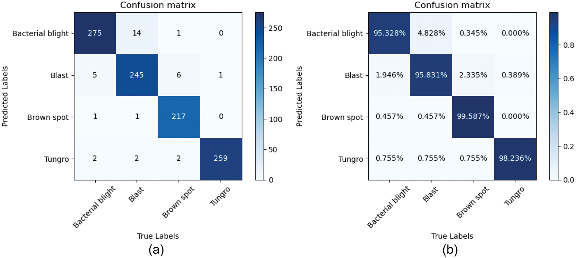
Figure 10: The GE-ShuffleNet confusion matrix. (a) Confusion matrix; (b) Normalized confusion matrix. The main diagonal (blue part) of the confusion matrix represents the correct prediction result, and the rest is the wrong identification

In addition, Precision, Recall, F1 score, and Accuracy are common evaluation indicators in classification tasks and will be used for further evaluation of our model performance. The Precision is shown in Eq. (4). As follows,

Precision=TPTP+FP(4)

Precision represents the probability that all the predicted positive samples are positive samples. TP (True Positive) represents the number of positive samples predicted to be positive, and FP (False Positive) indicates the number of negative samples predicted to be positive. Besides, (TP + FP) is the number of all predicted positive samples.

Recall refers to the probability that the actual positive samples are predicted to be positive samples. Therefore,

Recall=TPTP+FN(5)

where, False Negative (FN) represents the number of positive samples actually predicted to be negative, and (TP+FN) indicates the number of all actual positive samples. The F1-score takes into account the Precision and Recall at the same time, so that both can reach the highest. As follows,

F1−score=2⋅Precision⋅RecallPrecision+Recall(6)

Accuracy is an indicator widely used to evaluate models in deep learning. The higher the value, the better the performance of the model. Here,

Accuracy=TP+TNTP+TN+FP+FN(7)

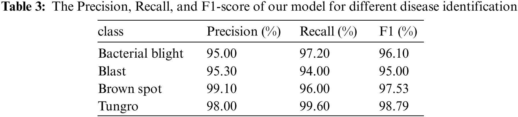
As shown in Table 3, the identification accuracy, recall rate, and F1-score of the proposed model for different diseases are recorded. We found that the classification precision of the four diseases was no less than 95%. Besides, the Precision and Recall of Brown spot and Tungro could reach 99.1% and 99.6%, respectively.

4.3 Performance Comparison of Different Models

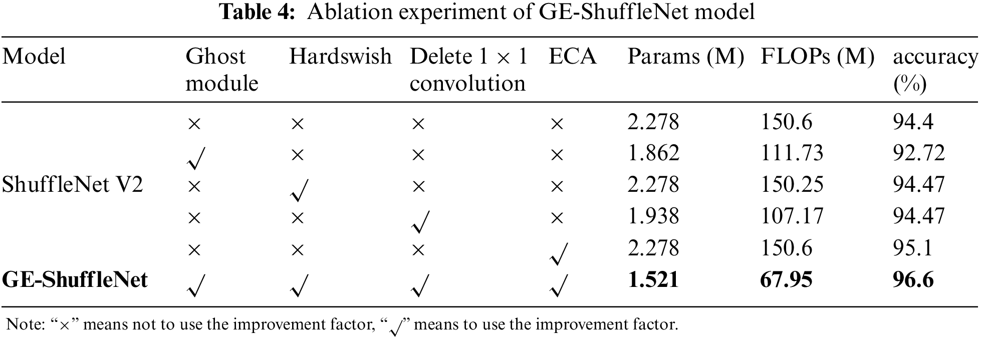
4.3.1 Ablation Test Results of the GE-ShuffleNet Model

To explore how to improve the performance of the ShuffleNet V2 model by using the Ghost module, Hardswish activation function, deleting 1×1 convolution of ShuffleNet V2 right branch and ECA attention mechanism, the ablation test was conducted and the results are described in Table 4. It can be seen from Table 4 that when the 1×1 convolution in the two basic units of ShuffleNet V2 is replaced by the Ghost module, the accuracy of the model decreases by 1.68%, but the Params and FLOP of the model decrease by 0.416 and 38.87 M, respectively. The Hardswish activation function is used to replace the ReLU activation function. When the model Params is unchanged, the FLOPs decrease slightly, and the accuracy of the model also increases slightly. The unimportant 1×1 convolution is deleted from the two basic unit modules of ShuffleNet V2. When the accuracy of the model increases, the model Params and FLOPs decrease by 0.34 and 43.43 M, respectively. The ECA attention mechanism structure is introduced into the two basic units of ShuffleNet V2, and the model accuracy is improved by 0.7% while keeping the model Params and FLOPs unchanged. By integrating the Ghost Module, Hardswish activation function, deleting the 1×1 convolution of the right branch of ShuffleNet V2, and improving ECA attention mechanism, the performance of the model has been greatly improved, the accuracy has been improved by 2.2%, Params reduced by 0.757 M, and the FLOPs has been reduced by 82.65 M. To more intuitively demonstrate the effectiveness of the GE-ShuffleNet model proposed in this study, the GE-ShuffleNet model will be compared with other different network models.

4.3.2 Performance Comparison between GE-ShuffleNet and Other Models

In this study, eight classical network models have selected for comparison to better highlight the advantages of the improved network in terms of precision and model parameters. As shown in (a) and (b) in Fig. 11, it is the comparison of the identification accuracy of GE-ShuffleNet, ShuffleNet V2, AlexNet, EfficienetNet V2 [39], MobileNet V2, ResNet50, Swim Transformer [40], GhostNet and VGG16 under different epochs. Figs. 11a and 11b correspond to the comparison of training and validation identification accuracy, respectively. By observing Fig. 11, the identification accuracy of different models increases with the increase of epochs. It should be noted that the identification accuracy of our model under different epochs is higher than that of other models. The results shown in Fig. 11 preliminarily confirm the performance of the proposed method. To further prove the advantages of the proposed model, Table 5 describes the accuracy, FLOPs, Params, and Model Size of different models.

Figure 11: The identification accuracy curve fitting results of different models under various epochs. (a) The comparison of training accuracy of different models; (b) The comparison of validation accuracy of different models

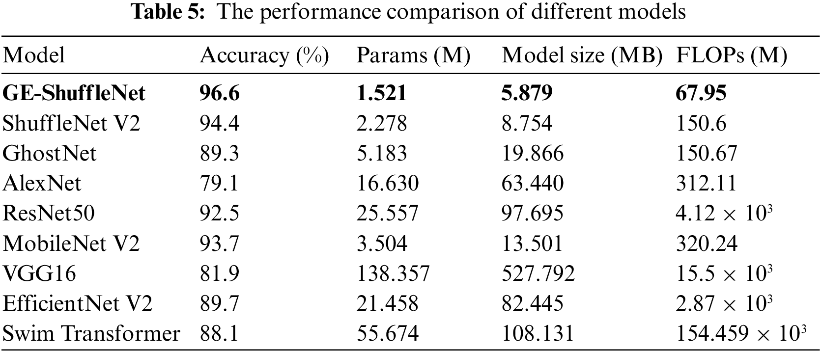
It can be seen from Table 5 that ShuffleNet V2 has higher accuracy (94.4%) than other models (MobileNet V2, GhostNet, AlexNet, Swim Transformer, EfficientNet V2, VGG16, and ResNet50). In addition, compared with these models, ShuffleNet V2 has obvious advantages in Params and Model Size. Then, compared with ShuffleNet V2, our model can not only improve the identification accuracy, but also reduce Params and model size. Especially, on the premise of reducing the model size to 2.875 MB, the identification accuracy of the proposed model is 2.2% higher than that of ShuffleNet V2. These quantitative comparison results highlight the advantages of the proposed model in disease identification and actual deployment.

5  Conclusion

In conclusion, this paper has proved the performance of GE-ShuffleNet through lots of experimental results. In our work, we first theoretically analyze the performance of ShuffleNet V2. A novel deep learning model is after that proposed to reduce the model size and improve accuracy for rice identification. The experimental results show that the identification accuracy with GE-ShuffleNet is more than ShuffleNet V2, MobileNet V2, GhostNet, AlexNet, Swim Transformer, EfficientNet V2, VGG16, and ResNet50. Moreover, compared with other models, GE-ShuffleNet is easier to deploy with fewer Params and smaller model sizes. This research provides an alternative method for intelligent spraying systems, intelligent disease diagnosis, and other equipment. In the future, we will further enrich the rice disease data set by collecting data from the experimental field to ensure the accuracy of the proposed model in practice.

Funding Statement: This work is supported in part by the Ji Lin provincial science and technology department international science and technology cooperation project under Grant 20200801014GH, and the Changchun City Science and Technology Bureau key science and technology research projects under Grant 21ZGN28.

Conflicts of Interest: The authors declare that we have no conflicts of interest to report regarding the present study.

References

1. J. Chen, D. Zhang, A. Zeb and Y. A. Nanehkaran, “Identification of rice plant diseases using lightweight attention networks,” Expert Systems with Applications, vol. 169, no. 4, pp. 114514, 2021. [Google Scholar]
2. P. K. Sethy, N. K. Barpanda, A. K. Rath and S. K. Beher, “Image processing techniques for diagnosing rice plant disease: A survey,” Procedia Computer Science, vol. 167, no. 1, pp. 516–530, 2020. [Google Scholar]
3. P. K. Sethy, N. K. Barpanda, A. K. Rath and S. K. B. MTech, “Deep feature based rice leaf disease identification using support vector machine,” Computers and Electronics in Agriculture, vol. 175, no. 1, pp. 105527, 2020. [Google Scholar]
4. Q. H. Cap, H. Tani, S. Kagiwada, H. Uga and H. Iyatomi, “LASSR: Effective super-resolution method for plant disease diagnosis,” Computers and Electronics in Agriculture, vol. 187, pp. 106271, 2021. [Google Scholar]
5. J. Feng, L. Yang, C. Yu, D. Cai and G. Li, “Image recognition of four rice leaf diseases based on deep learning and support vector machine,” Computers and Electronics in Agriculture, vol. 179, pp. 105824, 2020. [Google Scholar]
6. J. Parraga-Alava, K. Cusme, A. Loor and E. Santander, “RoCoLe: A robust a coffee leaf images dataset for evaluation of machine learning based methods in plant diseases recognition,” Data in Brief, vol. 25, no. 17, pp. 104414, 2019. [Google Scholar] [PubMed]
7. W. Ai, S. Liu, H. liao, J. Du, Y. Cai et al., “Application of hyperspectral imaging technology in the rapid identification of microplastics in farmland soil,” Science of The Total Environment, vol. 807, pp. 151030, 2022. [Google Scholar] [PubMed]
8. Y. Xiong, L. Liang, L. Wang, J. She and M. Wu, “Identification of cash crop diseases using automatic image segmentation algorithm and deep learning with expanded dataset,” Computers and Electronics in Agriculture, vol. 17, no. 4, pp. 105712, 2020. [Google Scholar]
9. D. Xiao, J. Feng, T. Lin, C. Pang and Y. Ye, “Classification and recognition scheme for vegetable pests based on the BOF-SVM model,” International Journal of Agricultural and Biological Engineering, vol. 11, no. 3, pp. 190–196, 2018. [Google Scholar]
10. Y. Shi, W. Huang, J. Luo, L. Huang and X. Zhou, “Detection and discrimination of pests and diseases in winter wheat based on spectral indices and kernel discriminant analysis,” Computers and Electronics in Agriculture, vol. 141, pp. 171–180, 2017. [Google Scholar]
11. J. Zhu, A. Wu, X. Wang and H. Zhang, “Identification of grape diseases using image analysis and BP neural networks,” Multimedia Tools and Applications, vol. 79, pp. 14539–14551, 2020. [Google Scholar]
12. A. K. Singh, A. Rubiya and B. S. Raja, “Classification of rice disease using digital image processing and svm classifier,” International Journal of Electrical and Electronics Engineers, vol. 7, no. 1, pp. 294–299, 2015. [Google Scholar]
13. L. Chen and Y. Yuan, “Agricultural disease image dataset for disease identification based on machine learning,” in Int. Conf. on Big Scientific Data Management, Cham, Springer, pp. 263–274, 2018. [Google Scholar]
14. U. K. Lopes and J. F. Valiati, “Pre-trained convolutional neural networks as feature extractors for tuberculosis detection,” Computers in Biology and Medicine, vol. 89, no. 7639, pp. 135–143, 2017. [Google Scholar] [PubMed]
15. S. Qiao, J. Li, C. Zhao and T. Zhang, “No-reference quality assessment for neutron radiographic image based on a deep bilinear convolutional neural network, nuclear instruments and methods in physics research section A: Accelerators,” Spectrometers Detectors and Associated Equipment, vol. 1005, no. 1, pp. 165406, 2021. [Google Scholar]
16. J. Yun, D. Jiang, Y. Sun, L. Huang, B. Tao et al., “Grasping pose detection for loose stacked object based on convolutional neural network with multiple self-powered sensors information,” IEEE Sensors Journal, (Early Accesspp. 1, 2022. [Google Scholar]
17. Y. Liu, D. Jiang, C. Xu, Y. Sun, G. Jiang et al., “Deep learning based 3D target detection for indoor scenes,” Applied Intelligence, vol. 25, no. 2, pp. 1–14, 2022. [Google Scholar]
18. C. R. Rahman, P. S. Arko, M. E. Ali, M. A. I. Khan, S. H. Apon et al., “Identification and recognition of rice diseases and pests using convolutional neural networks,” Biosystems Engineering, vol. 194, no. 1, pp. 112–120, 2020. [Google Scholar]
19. W. Zhou, H. Wang and Z. Wan, “Ore image classification based on improved CNN,” Computers and Electrical Engineering, vol. 99, no. 5–9, pp. 107819, 2022. [Google Scholar]
20. S. Dargan, M. Kumar, M. R. Ayyagari and G. Kumar, “A survey of deep learning and its applications: A new paradigm to machine learning,” Archives of Computational Methods in Engineering, vol. 27, no. 4, pp. 1071–1092, 2019. [Google Scholar]
21. Y. Kessentini, M. D. Besbes, S. Ammar and A. Chabbouh, “A two-stage deep neural network for multi-norm license plate detection and recognition,” Expert Systems with Applications, vol. 136, no. 3, pp. 159–170, 2019. [Google Scholar]
22. H. L. Sue, G. Hervé, B. Pierre and J. Alexis, “New perspectives on plant disease characterization based on deep learning,” Computers and Electronics in Agriculture, vol. 170, pp. 105220, 2020. [Google Scholar]
23. K. Thenmozhi and U. S. Reddy, “Crop pest classification based on deep convolutional neural network and transfer learning,” Computers and Electronics in Agriculture, vol. 164, no. 4, pp. 104906, 2019. [Google Scholar]
24. J. D. Chen, J. X. Chen, D. F. Zhang, Y. Sun and Y. A. Nanehkaran, “Using deep transfer learning for image-based plant disease identification,” Computers and Electronics in Agriculture, vol. 173, no. 2, pp. 105393, 2020. [Google Scholar]
25. C. R. Rahman, P. S. Arko, M. E. Ali, M. A. Iqbal Khan, S. H. Apon et al., “Identification and recognition of rice diseases and pests using convolutional neural networks,” Biosystems Engineering, vol. 194, no. 1, pp. 112–120, 2020. [Google Scholar]
26. Y. WU, “Identification of maize leaf diseases based on convolutional neural network,” Journal of Physics: Conference Series, vol. 1748, pp. 032004, 2021. [Google Scholar]
27. J. Suo, J. Zhan, G. Zhou, A. Chen, Y. Hu et al., “CASM-AMFMNet: A network based on coordinate attention shuffle mechanism and asymmetric multi-scale fusion module for classification of grape leaf diseases,” Frontiers in Plant Science, vol. 13, pp. 846767, 2022. [Google Scholar] [PubMed]
28. M. Lv, G. Zhou, M. He, A. Chen, W. Zhang et al., “Maize leaf disease identification based on feature enhancement and DMS-robust alexnet,” IEEE Access, vol. 8, pp. 57952–57966, 2020. [Google Scholar]
29. W. Zeng, H. Li, G. Hu and D. Liang, “Identification of maize leaf diseases by using the SKPSNet-50 convolutional neural network model,” Sustainable Computing: Informatics and Systems, vol. 35, pp. 100695, 2022. [Google Scholar]
30. P. K. Sethy, N. K. Barpanda, A. K. Rath and S. K. Behera, “Deep feature based rice leaf disease identification using support vector machine,” Computers and Electronics in Agriculture, vol. 175, no. 1, pp. 105527, 2020. [Google Scholar]
31. K. Han, Y. Wang, Q. Tian, J. Guo, C. Xu et al., “GhostNet: More features from cheap operations,” in Proc. of the IEEE/CVF Conf. on Computer Vision and Pattern Recognition (CVPR), Seattle, WA, USA, pp. 1580–1589, 2020. [Google Scholar]
32. N. Ma, X. Zhang, H. T. Zheng and J. Sun, “Shufflenet v2: Practical guidelines for efficient cnn architecture design,” in Proc. of the European Conf. on Computer Vision, Munich, Germany, European, pp. 116–131, 2018. [Google Scholar]
33. X. Zhang, X. Zhou, M. Lin and J. Sun, “Shufflenet: An extremely efficient convolutional neural network for mobile devices,” in Proc. of the IEEE Conf. on Computer Vision and Pattern Recognition, Salt Lake City, USA, pp. 6848–6856, 2018. [Google Scholar]
34. N. Ma, X. Zhang, H. T. Zheng and J. Sun, “Shufflenet v2: Practical guidelines for efficient cnn architecture design,” in Proc. of the European Conf. on Computer Vision, Munich, Germany, pp. 116–131, 2018. [Google Scholar]
35. S. Adyasha, K. D. Pradeep and M. Sukadev, “High accuracy hybrid CNN classifiers for breast cancer detection using mammogram and ultrasound datasets,” Biomedical Signal Processing and Control, vol. 80, no. Part 1, pp. 104292, 2022. [Google Scholar]
36. K. Han, Y. Wang, Q. Tian, J. Guo, C. Xu et al., “GhostNet: more features from cheap operations,” in Computer Vision and Pattern Recognition (CVPR), Seattle, WA, USA, IEEE, pp. 1580–1589, 2020. [Google Scholar]
37. Q. Wang, B. Wu, P. Zhu, P. Li, W. Zuo et al., “Supplementary material for “ECA-Net: Efficient channel attention for deep convolutional neural networks,” in Conf. on Computer Vision and Pattern Recognition (CVPR), Seattle, WA, USA, IEEE, pp. 13–19, 2020. [Google Scholar]
38. A. Howard, M. Sandler, G. Chu, L. C. Chen, B. Chen et al., “Searching for mobilenetv3,” in Proc. of the IEEE/CVF Int. Conf. on Computer Vision, Seoul, The Republic of Korea, pp. 1314–1324, 2019. [Google Scholar]
39. A. Waheed, M. Goyal, D. Gupta, A. Khanna, A. E. Hassanien et al., “An optimized dense convolutional neural network model for disease recognition and classification in corn leaf,” Computers and Electronics in Agriculture, vol. 175, no. 12, pp. 105456, 2020. [Google Scholar]
40. F. Wang, Y. Rao, Q. Luo, X. Jin, Z. Jiang et al., “Practical cucumber leaf disease recognition using improved swin transformer and small sample size,” Computers and Electronics in Agriculture, vol. 199, no. 2, pp. 107163, 2022. [Google Scholar]
Cite This Article
Copyright © 2023 The Author(s). Published by Tech Science Press.
This work is licensed under a Creative Commons Attribution 4.0 International License , which permits unrestricted use, distribution, and reproduction in any medium, provided the original work is properly cited.
Downloads
Citation Tools