Graph Construction Method for GNN-Based Multivariate Time-Series Forecasting

1  Introduction

Accurate predictions on multivariate time-series data (i.e., data with numerous input variables in a single step) are crucial for many real-world applications. For example, the spread of an infectious disease can be mitigated by predictions based on the infection status of surrounding areas [1], congested driving routes can be avoided with predictions based on traffic flow in different locations [2], and investment direction can be determined based on the stock price trend of various companies [3].

With the recent rapid development of machine/deep learning models, many deep learning models for multivariate time-series forecasting (MTSF) such as Recurrent Neural Networks (RNNs) have been proposed. Unlike conventional statistical models, RNNs are powerful for capturing nonlinear characteristics of temporal features within univariate time-series data (i.e., intra-series patterns) [4]. However, for an accurate MTSF, besides the intra-series patterns, inter-relationships between variables (i.e., inter-series patterns) should be considered because each variable depends not only on its own historical values, but also on the historical values of other variables. Hence, a recent trend to address this is to use Graph Neural Networks (GNNs), which learn both the intra-series and the inter-series patterns in the format of a graph [5–8].

In GNNs, a graph consists of nodes (entities or regions) and edges (interrelationships between nodes) [9], so setting an appropriate graph is important for modeling multivariate time-series data. The graph can be set in two ways. The first is to define a graph in advance based on location identification or distance-based neighbor node selection algorithm, which is called a pre-defined graph [10,11]. This works well for datasets with fixed edges, such as roads or flights connecting cities. However, this structure is not suitable for cases where the relationship between nodes changes dynamically, such as the economic growth rate and the number of confirmed infections by country [8,12]. In these cases, the graph must be continuously changed during training to reflect the relationships between nodes in the input data that change dynamically over time.

Therefore, many existing GNNs construct dynamically changed graphs based on the similarity between two nodes, such as embedding vector similarity [12] or attention score similarity [13]. However, there are three limitations to this approach.

1.    As time-series data is a combination of frequency functions, evaluation of their similarity must be made in the spectral domain where periodic patterns can be reflected fundamentally.

2.    Setting up a graph that only considers similarity cannot effectively represent the time delay between the two time-series data. Although the flow of the two data is similar, it is difficult to capture the similarity in the case of time delay.

3.    Existing GNN-based models consider all nodes equally weighted. There is no weighting process based on the number of connected nodes in the graph. However, hub nodes that are connected with many other nodes exchange more information than other nodes, so it is important to consider the influence of these hub nodes in constructing the graph.

To solve these limitations, in this paper, we propose a novel graph construction method for GNN-based MTSF models. The proposed method consists of three modules: (1) a Spectral Similarity Calculation Module to construct a graph based on the spectral features of the time-series data, (2) a Time Delay Reflection Module to refine the graph by considering the time delay between nodes, and (3) a Node Weighting Module to assign a weight to each node of the constructed graph according to the number of connections with other nodes. Using the proposed method, we obtain a graph matrix that contains the dynamic interrelationships between nodes that can enhance the forecasting performance of GNN-based MTSF models. In addition, we propose a forecasting model by replacing the graph construction part of a state-of-the-art GNN model by our graph construction method (hereafter, referred to proposed model). In extensive experiments on various public multivariate time series datasets, we show that the proposed graph construction method can improve the forecasting performance of existing GNN-based MTSF models, and the proposed prediction model can achieve up to 18.1% predictive performance improvement over the state-of-the-art model. Also, we visualize the constructed graph and show that our method can learn dynamic interrelationships between nodes. Finally, we investigate the effect of hyperparameters on our method and demonstrate that all components in our method are indispensable.

The contributions of this paper are as follows:

1.    We propose a graph construction method for GNN-based MTSF that reflects the relationship between nodes considering the similarity in a spectral domain, time delay, and hub node.

2.    We compare various MTSF models and demonstrate that our model outperforms other existing MTSF models in various public datasets.

3.    We prove that our graph construction method can enhance the forecasting accuracy of existing GNN-based MTSF models.

4.    We show that nodes with similar data patterns have high edge weight in a generated graph.

The paper is organized as follows. In Section 2, we describe the related works of the methodologies used in this paper and the time-series forecasting field. In Section 3, we introduce the problem formulation of this research. Section 4 describes the details of the model used in this paper. Experimental settings, datasets, and evaluation metrics are covered in Section 5. In Section 6, we introduce the experimental results. Finally, we summarize our work and discuss future studies in Section 7.

2  Related Works

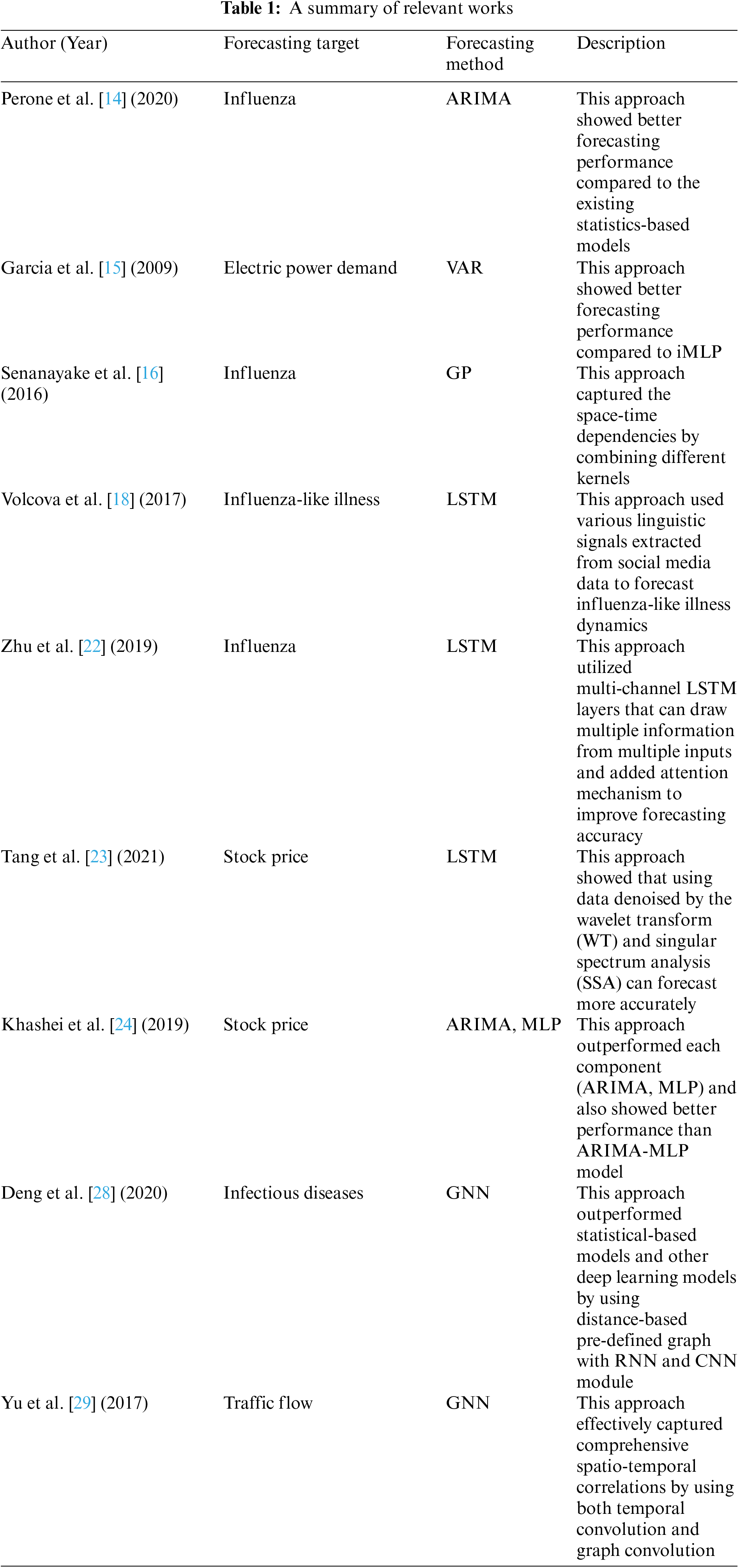
So far, diverse conventional statistical forecasting models have been used to forecast univariate time-series. For instance, Perone et al. [14] proposed the Auto Regressive Integrated Moving Average (ARIMA) model for forecasting future influenza outbreaks. They combined Auto Regression (AR) and Moving Average (MA) to show better forecasting performance compared to the existing statistical models. Furthermore, García-Ascanio et al. [15] proposed Vector Auto Regression (VAR) model, an extended model of the AR model, to capture the linear interdependencies among electric power time-series data. VAR achieved higher forecasting performance than interval Multi-Layer Perceptron (iMLP), a simple form of the neural network model. Senanayake et al. [16] proposed a non-parametric model based on Gaussian Process (GP) regression. GP model can be applied to multivariate time-series data by modeling multiple variables of a function using a Gaussian distribution. Accordingly, the GP regression model is applied to capture the spatial and spatial and temporal dependencies in influenza-like illness data. The model outperformed the predictive performance of the ARIMA model. However, these statistical forecasting models do not work well for rapidly changing multivariate time-series data [17]. This is because nonlinear relationships are not suitable for describing large datasets and focus on estimating mean values rather than data distributions.

Recently, deep learning models are demonstrating outstanding performance on MTSF. For instancec, Volkova et al. [18] proposed a long short-term memory (LSTM)-based deep learning model specialized for processing sequential time-series data [19–21] to forecast multivariate time-series data. They used topics, word n-grams, and stylistic patterns that were extracted from social media data. Zhu et al. [22] also proposed a LSTM-based deep neural model for influenza forecasting. The model had multi-channel LSTM layers that drew multiple pieces of information from multiple different inputs, including climate, pharmacy, and symptom data. Likewise, Tang et al. [23] proposed a LSTM-based deep learning model to predict stock prices. They denoised the data and passed the data through a model constructed by stacking LSTM in multiple layers. They improved the forecasting performance further by denoising. Khashei et al. [24] proposed a multi-layer perceptron (MLP)-based stock price forecasting model. They forecasted stock price through a hybrid model by combining ARIMA with MLP, and this model showed good performance compared to the existing statistical models [25].

Recently, GNN has been widely used for MTSF. The graph of GNN consists of a set of nodes representing each input variable in a multivariate time series and a set of edges representing the relationship between the input variables [26]. In GNN, node information is propagated through the edge, and prediction of a node is performed by considering information from neighboring nodes. GNNs are better suited for multivariate prediction because they can effectively reflect information from other nodes. GNN receives the graph as an input and learns along the relationship between nodes. Hence, they showed good performance in various areas.

Bloemheuvel et al. [27] proposed a GNN model that predicts peak ground acceleration (PGA), peak ground velocity (PGV), and spectral acceleration (SA) from seismic wave data from various locations in Italy. The features of each seismic wave were extracted through 1d convolutional neural network (CNN) layer, and each node information was exchanged through a Graph Convolutional Network (GCN). In addition, the authors set the adjacency matrix to be inversely proportional to the distance between nodes. The proposed model showed superior performance compared to the comparative models.

For instance, Deng et al. [28] forecasted the number of confirmed cases of infectious diseases using a distance-based pre-defined graph. In this model, the input time-series data is processed in parallel by the RNN and CNN modules. The RNN module obtains a hidden state with embedded temporal features for the input, and the model calculates an interrelationship attention score based on the hidden state value and the pre-defined graph. Meanwhile, the CNN module extracts temporal features by performing temporal convolution to the input data. Then, graph message passing is established based on interrelationship attention scores and temporal features obtained from the two modules. After that, the model predicts the node information through the MLP layer. The model outperformed statistical models and other deep learning models. On the other hand, Yu et al. [29] used both temporal convolution and graph convolution for traffic flow forecasting. Temporal convolution captures temporal features, and graph convolution captures inter-series patterns. The core of the model, the ST-Conv block, was constructed in the form of a graph convolution sandwiched between two temporal convolution layers. This ``sandwich" structure was created to achieve a bottleneck strategy for scale compression and feature squeezing with graph convolution. The model predicts traffic in each region through the input traffic data and a pre-defined road graph based on the distance between each area. Table 1 summarizes all the models mentioned so far.

However, graphs of existing GNN models have limitations in considering spectral similarity, time delay between nodes, and importance of hub nodes. In this paper, we propose a novel graph construction method that overcomes these limitations and construct a GNN-based MTSF model using the constructed graph. To consider spectral similarity, we utilize Fast Fourier transform (FFT) and to reflect the time delay, we identify the progress order of the two time-series data and reflect it in the graph. In addition, the weight of the hub node is increased by assigning a weight according to the number of connections each node has.

3  Problem Formulation

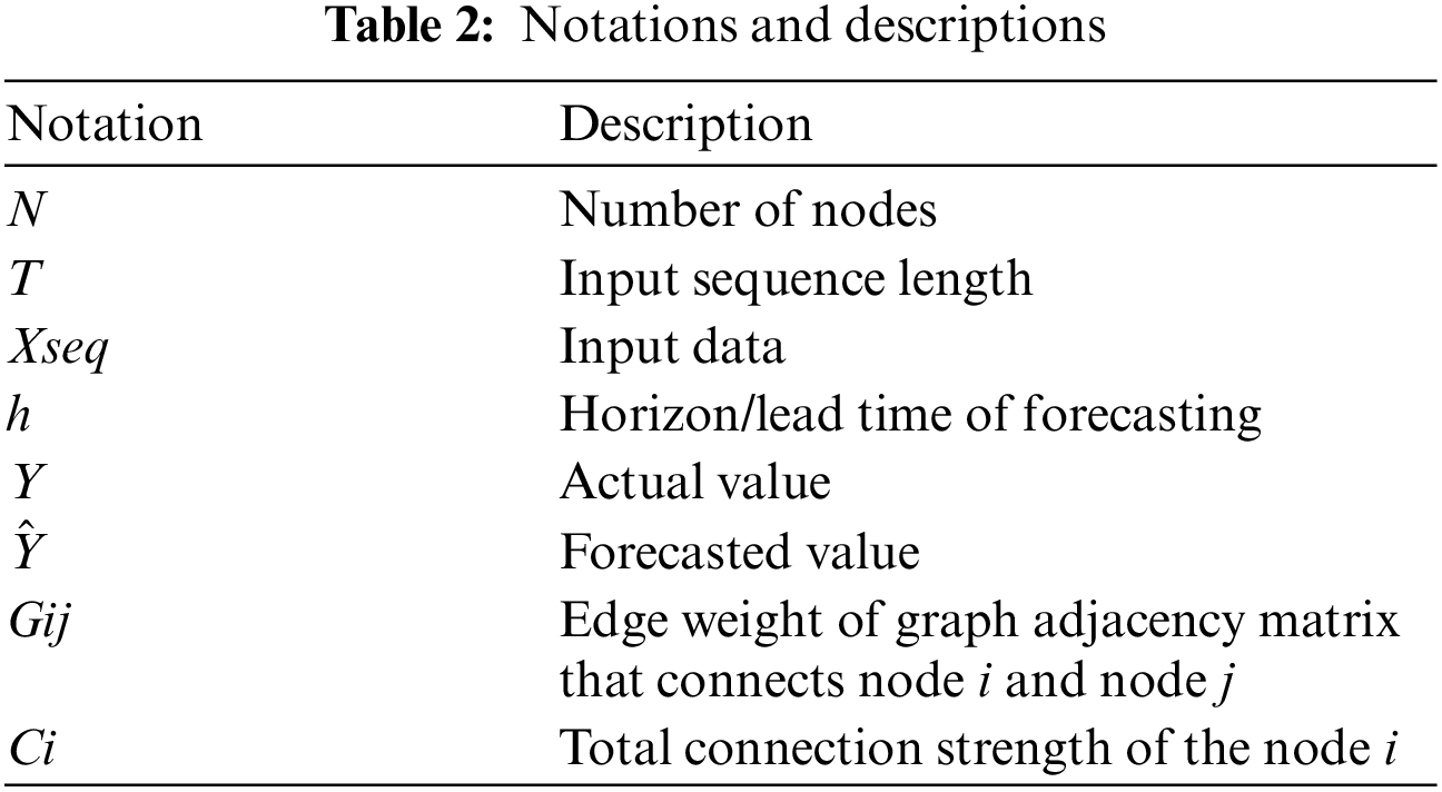
In this section, we first define a multivariate time-series forecasting problem based on a graph G. As described in Eq. (1), Xseq ={xti}∈RN×T stands for the multivariate time-series input, where N means the number of time-series (nodes), and T means the sequence length of input time-series data. Here, a node can be a region or city in influenza forecasting, a company in stock price forecasting, and a building or factory in electrical load forecasting. We denote xti∈R as time-series data in node i at time t, and indicate Xt = [xt1,xt2,xt3…xtN]∈RN×1 and Xi = [xt−T+1i,xt−T+2i,xt−T+3i…xti]∈R1×T as a set of time-series data in each node at time t and a set of node i during the past T time stamps, respectively. Our goal is to predict Y=[xt+h1,xt+h2,xt+h3…xt+hN], which is the value obtained after h time stamps. We denote by G the matrix representing connection information and interrelationships between multiple nodes. We also denote the edge weight of node i and node j in matrix G as Gij and the total connection strength of node i as Ci. Table 2 shows the key notations and descriptions. The undefined notations in this section are described in detail later.

Xseq=[xt−T+11⋯xt1⋮⋱⋮xt−T+1N⋯xtN](1)

4  Proposed Method

This section describes the overall structure of the proposed model. Fig. 1 shows the overall structure of our model.

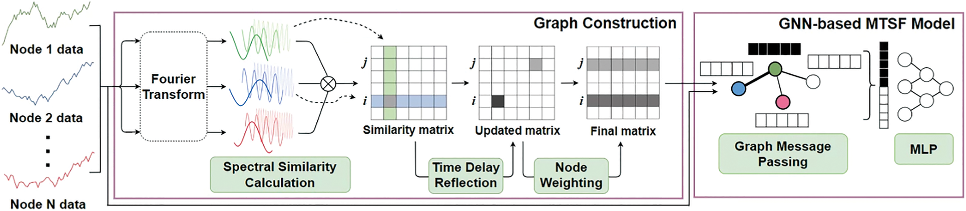
Figure 1: Overall architecture of the proposed method

4.1 Spectral Similarity Calculation Module

To determine the similarity of two time-series data, we compose the data into temporal frequencies and compare the intensity (amplitude) of each frequency to determine the similarity. FFT is a popular frequency decomposition technique for time-series data [30] due to its outstanding capability of learning latent representations of multiple time-series data in the spectral domain.

FFT decomposes a sequence data into multiple frequency components ranging from 1 to ⌊(T−1)/2⌋, about half of the input time length. Low-frequency functions represent the overall trend of the time-series data, while high-frequency functions represent the noise in the data [31]. Therefore, low-frequency functions are suitable for similarity comparison of time-series data. For this reason, we calculate the similarity of time-series in this layer using only low-frequency functions. We use the lower 20% of the frequency range, so the frequency range becomes 1 ~ ⌊⌊(T−1)/2⌋∗0.2⌋.

We calculate the similarity of the time-series data of two nodes using the decomposed frequency functions based on two factors: (1) The similarity of two time-series data is high when they have the same phase for the same frequency, and (2) the similarity is higher when the amplitudes of the two time series data are similar. To satisfy these factors, the similarity is calculated by dot-producting the amplitudes of low-frequency periodic functions of the two time-series data. Here, the similarity Gij of the time-series data of nodes i and j is calculated by Eqs. (2) and (3). In these equations, Ik and Jk represent the amplitude of k-th frequency function of Xi and Xj, which are the input time-series data of nodes i and j, respectively. In addition, t represents ⌊⌊(T−1)/2⌋∗0.2⌋, which is the highest frequency among the frequencies to be calculated.

After calculating the similarity of the time-series data between all nodes by Eq. (2), we can construct an N × N similarity matrix composed of Gij between nodes. The matrix values are arranged in normal distribution in order to filter values with high similarity. Similarity values with standard score greater than 0 are used, and values with standard score less than 0 are set to 0 to eliminate the edges.

FFT(Xi)≈∑k=1tIk, FFT(Xj)≈∑k=1tJk(2)

Gij=FFT(Xi)⋅FFT(Xj)(3)

4.2 Time Delay Reflection Module

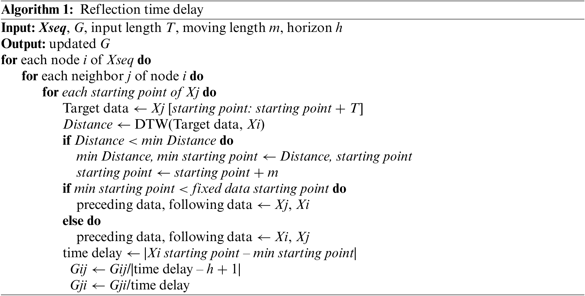
Although the Spectral Similarity Calculation Module constructs a similarity matrix in the spectral domain, various time-series data in the real world have a time delay. For example, in the case of infectious diseases, as the infectious disease spreads from the affected area, the number of confirmed cases in other areas (usually adjacent areas) also increases over time [32]. In this case, the current time series data has a great influence on subsequent time series data. In addition, data before h timestamp is most important when forecasting after h timestamp. Such time delay property of the time series data is handled by the Time Delay Reflection Module, as described in Algorithm 1. In particular, the algorithm considers two factors: One is the time delay and the other is the horizon difference. To account for time delay, we set one of the two time-series data as fixed data and the other as moving data. Then, while moving the starting point of the moving data, we find the point where the distance between the two time-series data is minimal. Here, the distance is calculated using Dynamic Time Warning (DTW) [33], an algorithm that measures the similarity between two time-series data. DTW is easier to eliminate noise than Euclidean distance because it uses not only the same time data but also the surrounding time data as a comparison target. If the DTW distance is the minimum at the point where the starting point of the moving data is smaller than the starting point of the fixed data, we set the moving data as the preceding data. In addition, we consider horizon time step h when constructing the graph. To do this, we set Gij large when the temporal difference (time delay) between the data at preceding node i and the data at following node j is exactly h, and set smaller when the temporal difference is far from h. Accordingly, the edge weight is set to be inversely proportional to the absolute value of the difference between horizon time step and time delay. If the time delay is equal to the horizon time step, then the weight Gij of the edge connecting two nodes i and j is set to 1. The graph edge weight from the following node to the preceding node is set to be inversely proportional to the time delay.

4.3 Node Weighting Module

In dynamically changing data such as population movement or economic flow, the influence of hub nodes with many connected edges such as amount of movement is much greater than that of other ordinary nodes. For example, hub airports with many transfers are crowded with transfer passengers [34]. Therefore, it is important to reflect hub node information to the graph for the GNN model to learn dynamically changing data. To do that, we assigned a higher weight to nodes with many connections with other nodes.

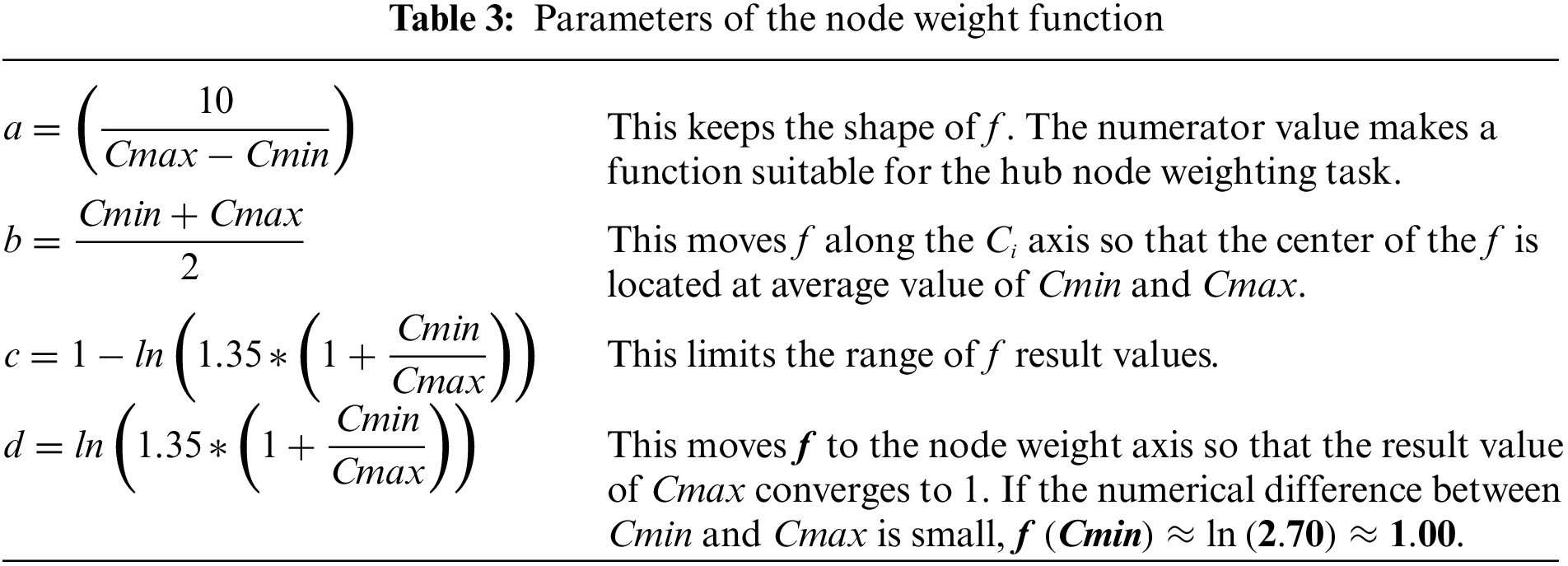
Earlier, we constructed a graph G that defined the edge weights of the graph based on the similarity between nodes. The goal of this module is to reflect the weights according to the influence of nodes on the graph using Eq. (4). In the equation Ci represents the total amount of influence node i has and f represents a transformation function with the similarity value calculated in the earler step. Then, we update the original graph Gi by multiplying f(Ci) to obtain the updated Gi. We multiplied edges from a node with a lower weight to another node by a lower weight. Conversely, we multiplied the edges from the node with a higher weight to another node by a higher weight.

Giupdated=f(Ci)⋅Gioriginal(4)

If we denote the sum of the influences node i has on its neighboring nodes as Ci, C={C1,C2,C3,…Cn}. Eq. (5) describes how to calculate Ci. Here, Ni denotes the set of neighboring nodes of node i. If we use the original similarity value in this step, the influence of nodes with few connections can be completely removed. Hence, we applied a logarithmic function to the similarity so that small similarity values are not removed and have only minimal impact. Also, we set all Cis to be positive based on the largest and smallest connection weights, Cmax and Cmin, respectively.

Ci=∑j∈Ni(ln(Gij+1)+1)(5)

f(Ci)=(11+e−a∗(Ci−b))∗c+d(6)

We generate a node weighting function f via Ci, and multiply f by Goriginal. In this way, we update Goriginal by applying node weight. We define the function f as Eq. (6). This function determines the weight for each node, such that hub nodes are given large weights. We describe the explanation of parameter a ~ d in Table 3 that used in Eq. (6) to eliminate differences in expressions according to data characteristics. The node weight was multiplied by the row corresponding to each node of the Goriginal. We repeat this process for all nodes and obtain the Gupdated.

4.4 GNN-Based MTSF Model

Using the graph constructed by the proposed method, we construct a GNN-based MTSF model (referred to “the proposed model” in the following sections) based on Cola-GNN [28]. This model was initially proposed for predicting infectious disease occurrences and used a pre-defined graph that considered only geological locations. We modified this pre-defined graph structure using the proposed graph construction method so that the graph can reflect dynamically changing interrelationships between the variables (nodes). Even though we apply our graph to Cola-GNN for forecasting, our graph structure can be applied to other GNN-based models (described in Section 6. D).

Now, we describe the process of learning the inter-relationship and the intra-relationship of multivariate time-series using the graph we proposed. Cola-GNN consists of three main components: (1) graph that considers inter-relationships between nodes, (2) node feature that represents the intra-relationship in each node, and (3) graph message passing that uses graph and node feature for learning information from neighboring nodes. We obtain the first component by attention score based on the last hidden state of the RNN. Then, we use this attention matrix along with the graph G generated by the graph construction layer. Next, we obtain the features of each node by applying dilated convolution to each node of Xseq. Finally, we perform graph message passing and forecast future time-series with neighbor nodes data.

5  Experimental Settings

To evaluate the effectiveness of the proposed model, we performed extensive experiments using six public datasets. Before we present the experimental results in detail, we first describe the datasets we used, the evaluation metrics, and the experimental setup for the comparison models.

5.1 Datasets

We used six real-world datasets in the experiments: three influenza-like illness (ILI) data, exchange rate data, stock price data, and electrical load data. In the experiments, we normalized all datasets to a range between 0 and 1 for each node data using min-max normalization. Also, we split the data into training, validation, and test sets in chronological order at ratios of 60%, 20%, and 20%.

•   ILI US-States: This contains weekly ILI for each state in the US from 2010 to 2017. From the original dataset, we utilized weekly data on new cases in each state in the United States from the Centers for Disease Control and Prevention (CDC) [35].

•   ILI US-Regions: This dataset includes weekly ILI for ten regions of the US from 2002 to 2017. The ten regions were defined as geographically close states by the Department of Health and Human Services (HHS). Data collection proceeded in the same way as US-States.

•   ILI Japan-Prefectures: This contains weekly ILI for each prefecture in Japan from 2012 to 2019. We collected weekly data on new cases in each prefecture in Japan from the Infectious Diseases Weekly Report (IDWR) [36].

•   Exchange rate: This contains daily exchange rate data for 8 countries (Australia, British, Canada, Switzerland, China, Japan, New Zealand, and Singapore) from 1990 to 2016 [37].

•   US stock market price: We collected daily stock prices of 50 major companies listed on the US stock market from 2007 to 2016 [38] and composed this dataset.

•   GEFCOM 2012: This dataset includes the hourly electrical load data of a US utility from January 1, 2005 to December 31, 2008 for 20 zones, which were used in the load forecasting track of the Global Energy Forecasting Competition 2012 (GEFCOM 2012) hosted on Kaggle [39]. Among 20 zones, we utilized data from zone 1 to zone 11 since the other nine zones have different variable conditions.

5.2 Evaluation Metrics

RMSE=1N∑i=1N(y^i−yi)2(7)

PCC=∑n=1N(yi¯−yi)(y^i¯−y^i)∑n=1N(yi¯−yi)2∑n=1N(y^i¯−y^i)2(8)

For performance comparison, we used two popular metrics for MTSF [28]: Root Mean Squared Error (RMSE) and Pearson Correlation Coefficient (PCC). The RMSE represents the difference between forecasted values and actual values. PCC is a numerical value in range (−1, 1) that quantifies the linear correlation between forecasted and actual values. Since PCC is calculated as a value close to 1 when the predicted value is similar to the actual value, it is useful not only for comparison between different models but also for comparison between different datasets. On the other hand, RMSE is represented by a lower value as the model’s forecasting performance improves, and is not suitable for comparing the predictive performance of different datasets due to data scale dependence. We selected these two metrics because PCC is easy to compare since all results are calculated in the same range, and RMSE is effective in determining how far the predicted value differs from the actual value.

We denote the forecasted values, actual values, and number of data samples as y^i, yi, and N, respectively. We also denote the mean value of yi as yi¯. RMSE and PCC are calculated using Eq. (7) [40] and (8) [41,42], respectively.

5.3 Experimental Settings

For performance comparison, we considered eight different MTSF models: AutoRegressive (AR), AutoRegressive and MovingAverage (ARMA), MLP, RNN, LSTM, LSTNet, ST-GCN, and Cola-GNN. We set epoch, batch size, learning rate, input sequence length T, and dropout probability to 500, 100, 0.001, 30, and 0.3 respectively. And we measure the forecasting performance by averaging the results of repeating the experiment 5 times. Depending on the setting of the [28], we evaluate our approach in short-term (horizon h = 2, 3) and long-term (horizon h = 5, 10, 15) settings. We ignore the case of h equals 1 because symptom monitoring data is usually delayed by at least one-time step. We measured the forecasting performance by averaging the results of repeating the forecasting 10 times. All experiments were done in the Python environment, and all models were implemented using PyTorch [43] library. The model-specific hyperparameters are empirically determined.

6  Experiments and Discussion

In this section, we first present the experimental results and analyze the graph we construected. We then report on the ablation studies performed.

6.1 Forecasting Performance

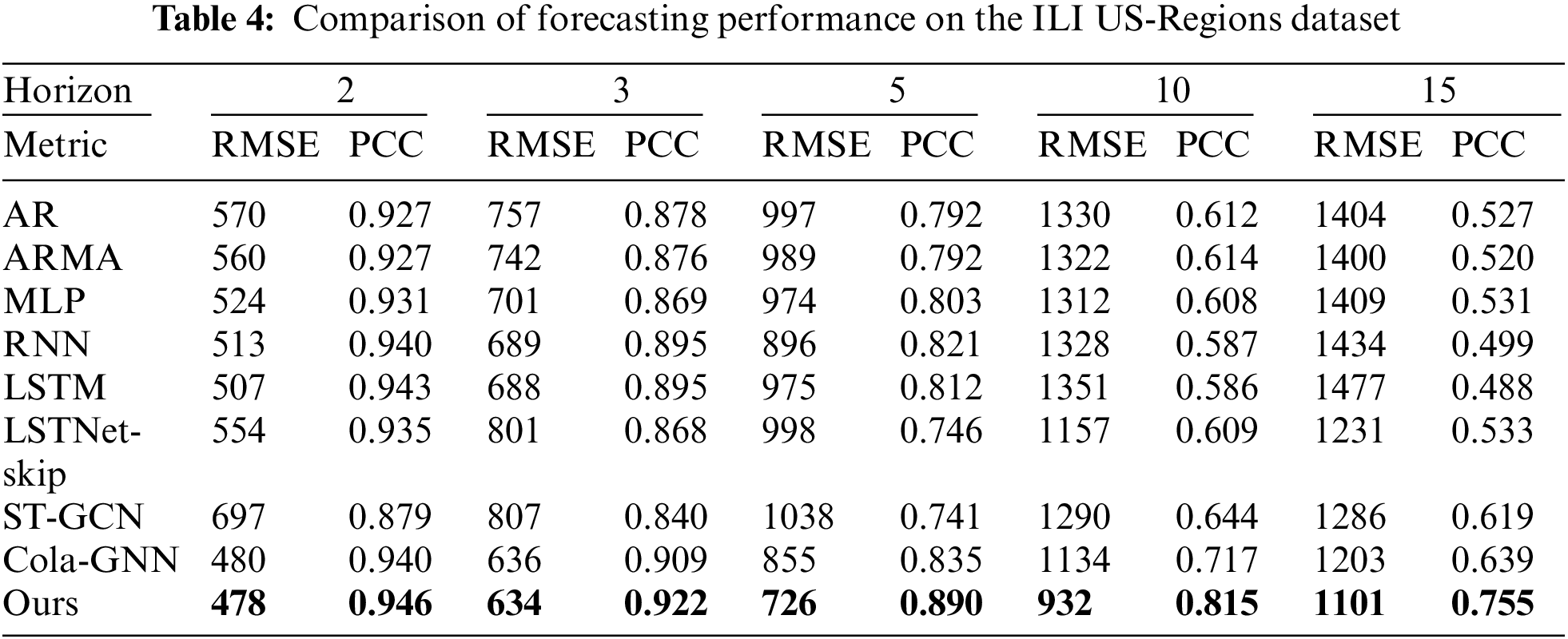
Tables 4–9 show the results of comparative experiments using six datasets. In the tables, the bold values indicate the highest values of RMSE and PCC in each horizon. Tables 4–6 present the results of comparative experiments on the ILI datasets. Table 4 shows that our model outperforms other existing models for all cases on the ILI US-Regions dataset. In particular, since the graph generated by the proposed model better reflects the characteristics of dynamically changing time series data than the predefined graph of Cola-GNN, the proposed model shows better predictive performance.

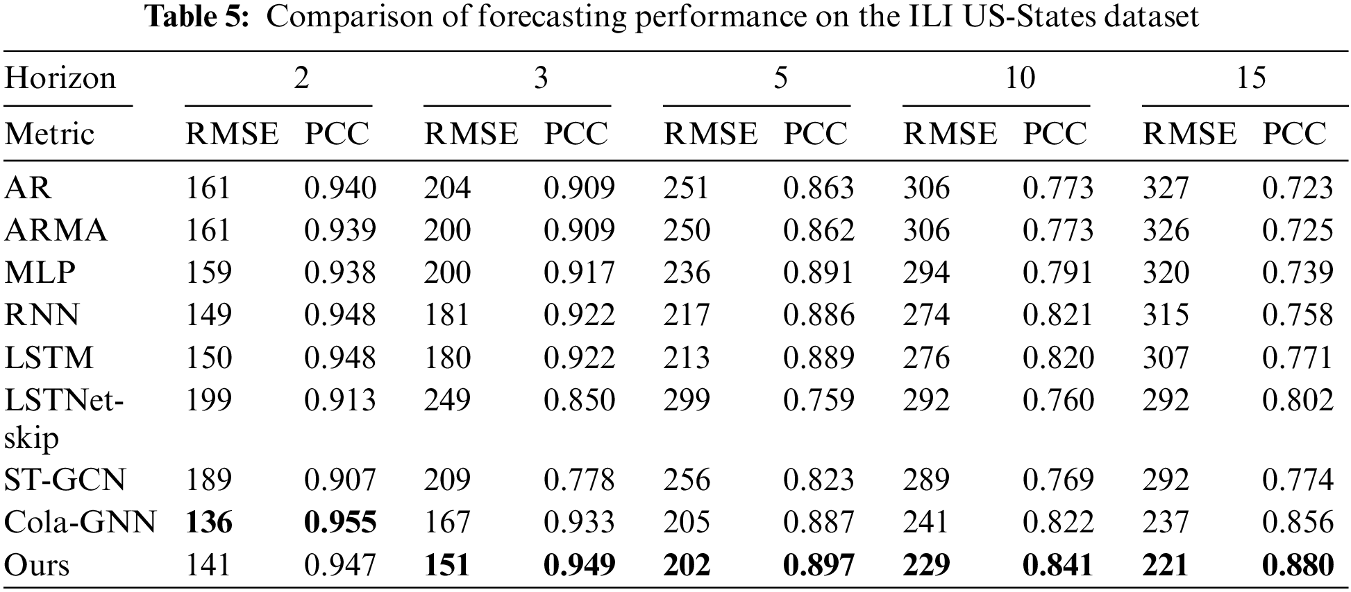
On the other hand, Table 5 for the ILI US-States dataset shows that the proposed model achieves the best accuracy, except for h = 2 and 5, where Cola-GNN had the best predictive performance. Even in these cases, our model achieves the second best performance, and the difference from the best case is negligible compared to the other models. This is because ILI US-States dataset has a more fine-grained pre-defined graph (51 nodes) compared to the ILI US-Regions dataset (10 nodes). As a result, in some cases, the Cola-GNN model performed better on the ILI US-tates dataset.

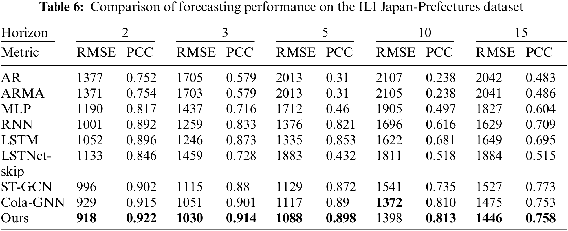
In Table 6 for the ILI Japan-Prefectures dataset, our model outperforms other models in all cases except when h = 10 in RMSE. However, our model achieves the best performance in PCC.

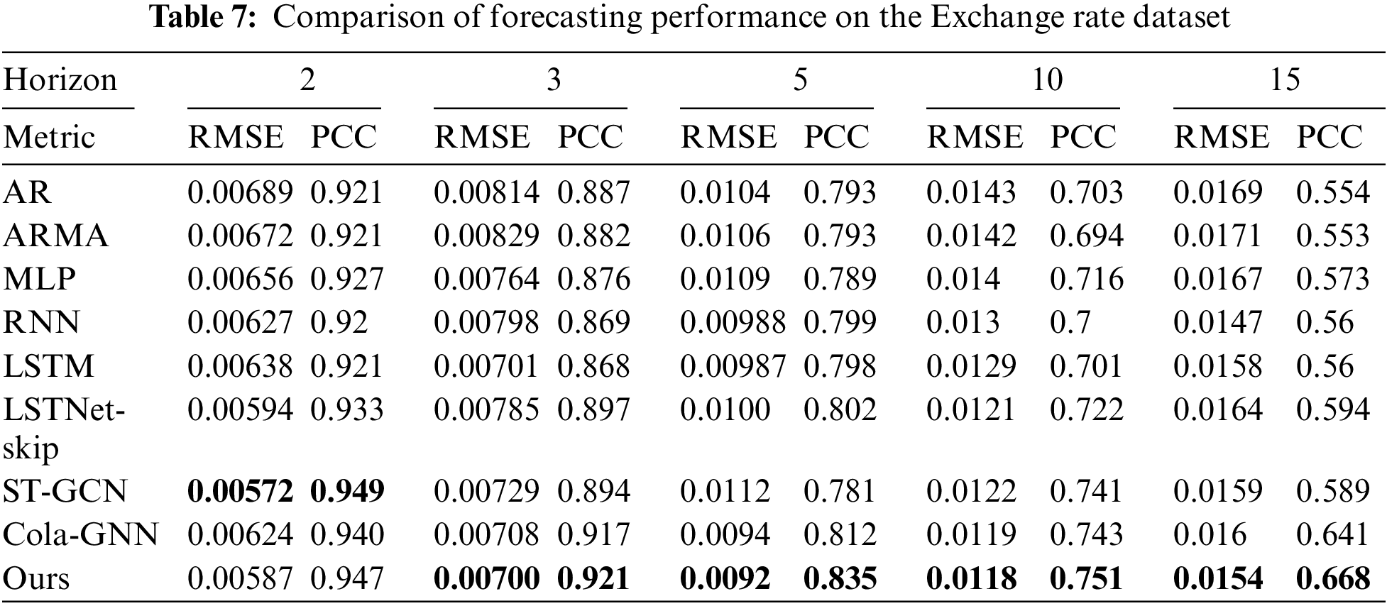
Table 7 presents the comparison results for the Exchange rate dataset, similar to the results for the ILI US-States dataset. It should be noted that ST-GCN performs well when h = 2 in this experiment. This is because unpredictable factors such as the international situation are more decisive than trends in time series data for short-term forecasting in the economic field [44]. Therefore, the effectiveness of our proposed graph construction may be reduced for short-term forecasting. Nevertheless, our model shows the best performance in other cases.

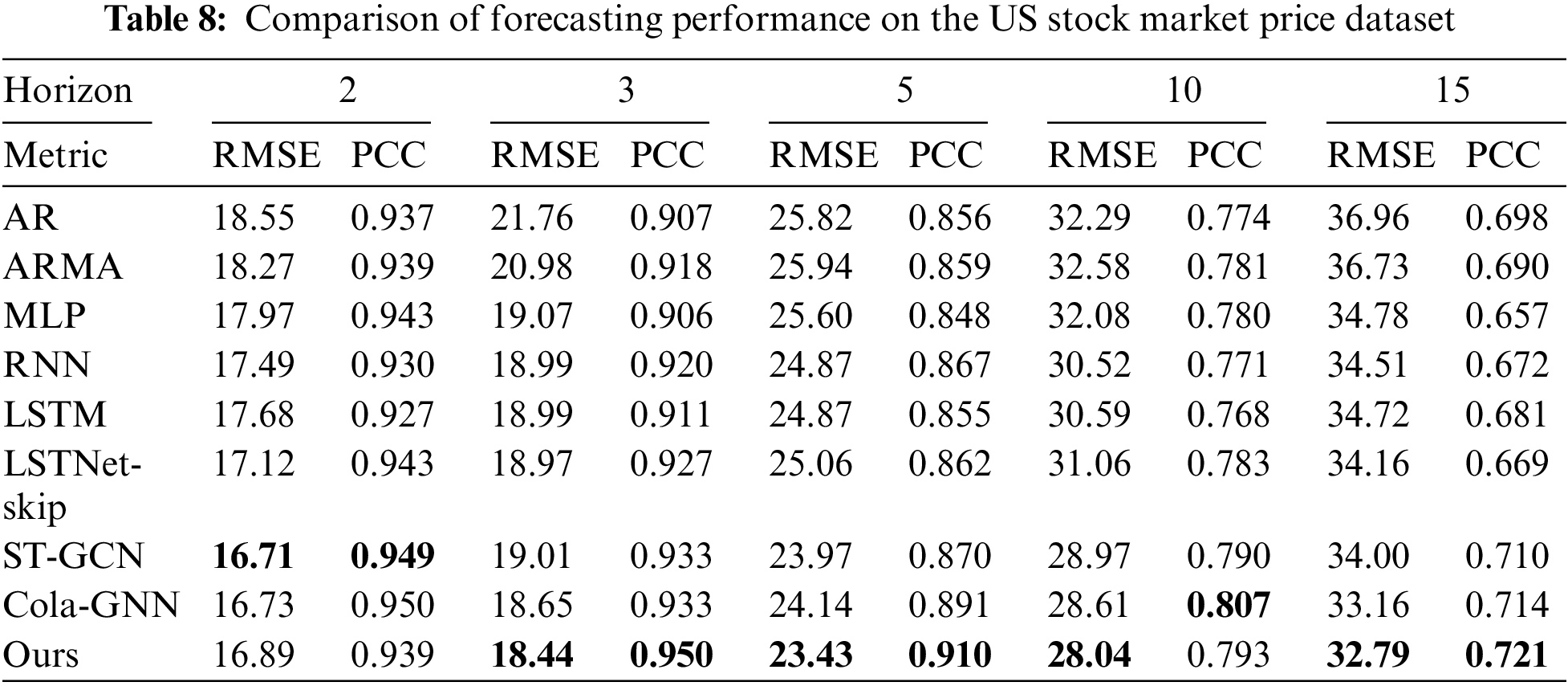
Table 8 presents the results for the US stock market price dataset, similar to the results of the Exchange rate dataset. Our model shows slightly lower performance for US stock market dataset compared to the Exchange rate dataset. This is because the US stock market price data set has less influence on each other than the Exchange rate dataset.

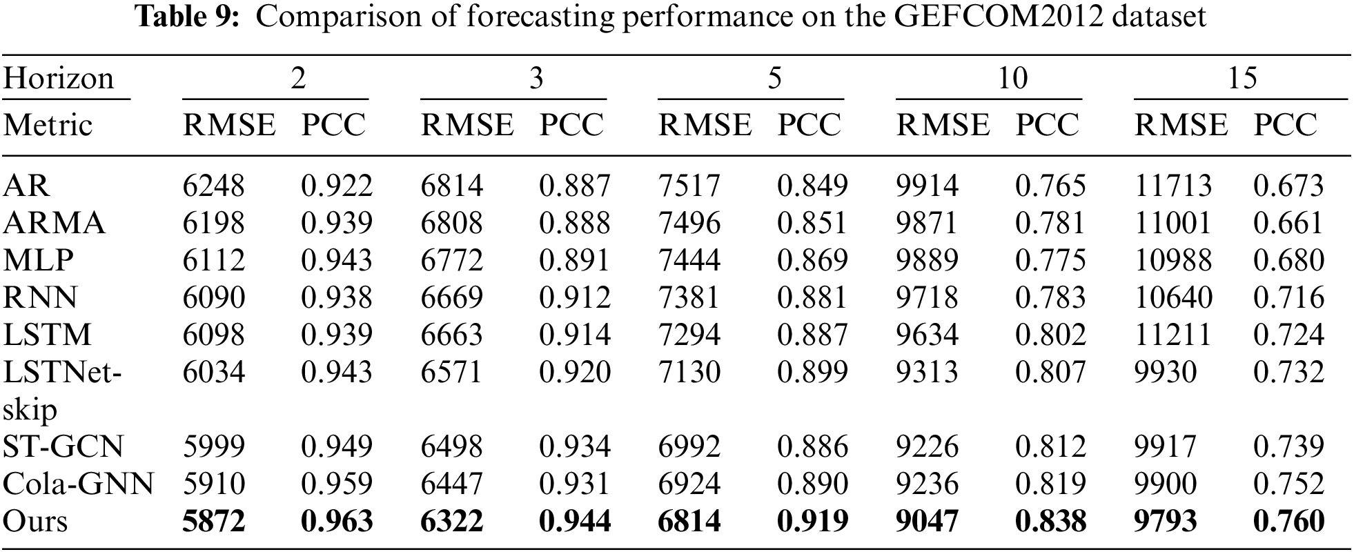
Lastly, Table 9 (GEFCOM 2012 dataset) shows that our model achieved the best accuracy for all cases. Also, Cola-GNN ranked second in most cases. Statistics-based forecasting models showed relatively low performance than GNN-based forecasting models. In addition, our model showed outstanding performance even in multi-regional electrical load forecasting.

To sum up, our model showed the best performance in most cases (21 out of 25 for RMSE and 20 out of 25 for PCC). Also, basic deep learning models (MLP, RNN, LSTM) exhibited better accuracy than statistical models (AR, ARMA). However, GNNs (ST-GCN, Cola-GNN, our model) showed higher performance than basic deep learning models. Particularly, our model showed outstanding performance, in the long-term forecasting that has a large difference between the test period and training period, compared to short-term forecasting.

6.2 Graph Analysis

In this section, we present analysis results through comparison with the input data to provide a more intuitive understanding of the constructed graph.

Fig. 2a exhibits a heat map that visually represents the edge weights of New York (NY) state and other states when forecasting the future ILI occurrence in NY when h = 10, using the ILI US-State data. Fig. 2b shows the actual ILI for the states with high similarity to NY, such as New Jersey (NJ), Massachusetts (MA), and Pennsylvania (PA). In Fig. 2a, the red color of the state indicates a higher edge weight, and white color indicates a lower edge weight. Since infectious disease diffusion is greatly affected by geographical factors (e.g., distance from the origin), nearby states of NY show higher edge weight. For instance, NJ and MA, which are close to NY, have high edge weights. Conversely, states that are far away from NY, such as Florida (FL), have low edge weights. From this visualization, we can observe that the graph generated by the proposed method reflects the relationship between nodes well. In Fig. 2b, we can also observe that the occurrences trend and peak timing of ILI are almost identifical in NY and the states with high edge weights.

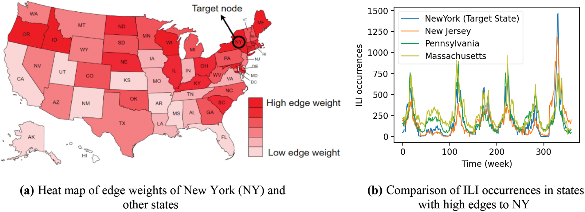
Figure 2: Visualization of similar nodes when forecasting NY in ILI US-States data

As a result, our model has good interpretability because it shows good performance in capturing interrelationships and can visually represent the results.

6.3 Ablation Study

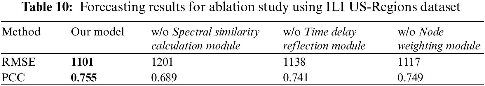
To analyze the effect of each component in our model, we conducted some ablation tests using ILI US-Regions dataset. We compare the performance of the following three methods using the ILI US-Regions dataset when h = 15.

•   w/o Spectral Similarity Calculation Module: Instead of the graph generated by the Spectral Similarity Calculation Module, we just use the pre-defined graph of Cola-GNN.

•   w/o Time Delay Reflection Module: Here, we do not use the Time Delay Reflection Module. That is, we just pass the outputs of the Spectral Similarity Calculation Module to the next Node Weighting Module directly.

•   w/o Node Weighting Module: Here, we do not perform the node weighting. That is, we pass the generated graph to the Forecasting part without refining the node weights depending on the connectivity.

Table 10 shows the RMSE and PCC of the three methods. The results show that all components of our model are contributing to improved performance. First, the Spectral Similarity Calculation Module significantly improves the performance because it creates a graph based on spectral similarity, enabling efficient information flow between nodes. Furthermore, the second method demonstrates that incorporating time order and time delay into the graph help improve performance. Lastly, the Node Weighting Module shows the advantage of reflecting the importance of the hub nodes in the graph. That is, the information passing through the hub nodes has a lot of influence on the performance.

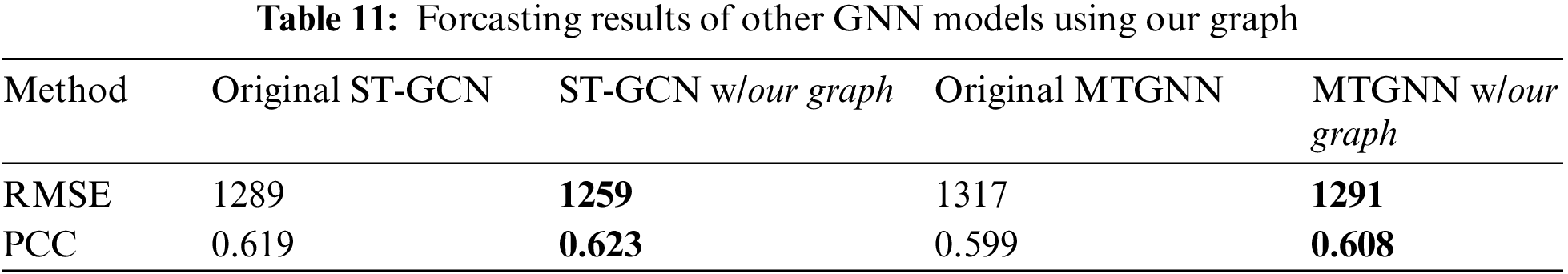
6.4 Applicability of the Graph Construction Method

In this section, we analyze the applicability of our graph method to other GNNs. Even though we used Cola-GNN for prediction, our graph can be applied to other GNNs. To demonstrate this, we consider ST-GCN [29] and MTGNN [12] for forecasting. Table 11 shows their forecasting results on the ILI US-Regions dataset. In the table, both models showed better forecasting performance using the proposed graph.

7  Conclusion

In this paper, we proposed a novel graph construction method for GNN-based MTSF models. For effective graph construction, we considered spectral similarity between nodes, time-delay between time-series data of each node, and weight of hub nodes. We then constructed a MTSF model based on Cola-GNN using the constructed graph. To demonstrate the effectiveness of the proposed method, we compared the proposed model with other existing forecasting models in terms of RMSE and PCC using public datasets from various fields (e.g., infectious disease, exchange rate, and stock market data). Experimental results show that our model outperforms other comparative models in most cases, especially in long-term forecasting.

We also conducted ablation tests to verify the importance of each component in the proposed method. Experimental results show that all the components in the proposed method are indispensable. In addition, we showed that the proposed model has an advantage of interpretability through the visualization of the interrelationships between nodes. In the analysis of the heat map representing node similarity, it was confirmed that the proposed model effectively captures the interrelationships between nodes.

Even though our model outperforms other models, the accuracy of short-term forecasting is still unsatisfactory compared to long-term forecasting. In addition, in node weighting process, forecasting accuracy can be improved further by optimizing the parameters that adjust the node weighting function. In future works, we will consider a graph that fits the characteristics of different time-series data and optimize the best parameters for node weighting to improve short-term forecasting performance.

Funding Statement: This research was supported by Energy Cloud R&D Program (grant number: 2019M3F2A1073184) through the National Research Foundation of Korea (NRF) funded by the Ministry of Science and ICT.

Conflicts of Interest: The authors declare that they have no conflicts of interest to report regarding the present study.

References

1. C. Jinming, X. Jiang and B. Zhao, “Mathematical modeling and epidemic prediction of COVID-19 and its significance to epidemic prevention and control measures,” Journal of Biomedical Research & Innovation, vol. 1, no. 1, pp. 1–19, 2020. [Google Scholar]

2. J. Barros, M. Araujo and R. J. F. Rossetti, “Short-term real-time traffic prediction methods: A survey,” in Proc. of the Int. Conf. on Models and Technologies for Intelligent Transportation Systems (MT-ITS), Budapest, Hungary, pp. 132–139, 2015. [Google Scholar]

3. J. G. Agrawal, V. Chourasia and A. Mittra, “State-of-the-art in stock prediction techniques,” International Journal of Advanced Research in Electrical, Electronics and Instrumentation Engineering, vol. 2, no. 4, pp. 1360–1366, 2013. [Google Scholar]

4. H. Y. Cheng, Y. C. Wu, M. H. Lin, Y. L. Liu, Y. Y. Tsai et al., “Applying machine learning models with an ensemble approach for accurate real-time influenza forecasting in Taiwan: Development and validation study,” Journal of Medical Internet Research, vol. 22, no. 8, pp. e15394, 2020. [Google Scholar] [PubMed]

5. Y. Wang and T. Aste, “Sparsification and filtering for spatial-temporal GNN in multivariate time-series,” arXiv preprint: 2203.03991, 2022. [Google Scholar]

6. D. Cheng, F. Yang, S. Xiang and J. Liu, “Financial time series forecasting with multi-modality graph neural network,” Pattern Recognition, vol. 121, pp. e108218, 2020. [Google Scholar]

7. Y. Cui, K. Zheng, D. Cui, J. Xie, L. Deng et al., “METRO: A generic graph neural network framework for multivariate time series forecasting,” in Proc. of the VLDB Endowment, Copenhagen, Denmark, vol. 15, no. 2, pp. 224–236, 2021. [Google Scholar]

8. D. Cao, Y. Wang, J. Duan, C. Zhang, X. Zhu et al., “Spectral temporal graph neural network for multivariate time-series forecasting,” in Proc. of the Advances in Neural Information Processing Systems, Virtual Conference, vol. 33, pp. 17766–17778, 2020. [Google Scholar]

9. Z. Wu, S. Pan, F. Chen, G. Long, C. Zhang et al., “A comprehensive survey on graph neural networks,” IEEE Transactions on Neural Networks and Learning Systems, vol. 32, no. 1, pp. 4–24, 2020. [Google Scholar]

10. Z. Chen, M. Dehmer and Y. Shi, “A note on distance-based graph entropies,” Entropy, vol. 16, no. 10, pp. 5416–5427, 2014. [Google Scholar]

11. M. Xie, H. Yin, H. Wang, F. Xu, W. Chen et al., “Learning graph-based poi embedding for location-based recommendation,” in Proc. of the ACM Int. Conf. on information and Knowledge Management, Indiana, USA, pp. 15–24, 2016. [Google Scholar]

12. Z. Wu, S. Pan, G. Long, J. Jiang, X. Chang et al., “Connecting the dots: Multivariate time series forecasting with graph neural networks,” in Proc. of the ACM SIGKDD Int. Conf. on Knowledge Discovery & Data Mining, California, USA, pp. 753–763, 2020. [Google Scholar]

13. P. Veličković, G. Cucurull, A. Casanova, A. Romero, P. Liò et al., “Graph attention networks,” in Proc. of the Int. Conf. on Learning Representations, Vancouver, Canada, pp. 1–12, 2017. [Google Scholar]

14. G. Perone, “An ARIMA model to forecast the spread of COVID-2019 epidemic in Italy,” arXiv: 2004.00382, 2004. [Google Scholar]

15. C. García-Ascanio and C. Maté, “Electric power demand forecasting using interval time-series: A comparasion between VAR and iMLP,” Energy Policy, vol. 38, no. 2, pp. 715–725, 2009. [Google Scholar]

16. R. Senanayake, S. O’Callaghan and F. Ramos, “Predicting spatio-temporal propagation of seasonal influenza using variational gaussian process regression,” in Proc. of the Conf. on Artificial Intelligence, Arizona, USA, vol. 30, no. 1, 2016. [Google Scholar]

17. E. Spiliotis, S. Makridakis, A. A. Semenoglou and V. Assimakopoulos, “Comparison of statistical and machine learning methods for daily SKU demand forecasting,” Operational Research, vol. 22, no. 3, pp. 3037–3061, 2020. [Google Scholar]

18. S. Volkova, E. Ayton, K. Porterfield and C. D. Corley, “Forecasting influenza-like illness dynamics for military populations using neural networks and social media,” PLoS One, vol. 12, no. 12, pp. e0188941, 2017. [Google Scholar] [PubMed]

19. B. Chakravarthi, S. C. Ng, M. R. Ezilarasan and M. F. Leung, “EEG-based emotion recognition using hybrid CNN and LSTM classification,” Frontiers in Computational Neuroscience, vol. 16, pp. 1–9, 2022. [Google Scholar]

20. S. Jung, J. Moon, S. Park and E. Hwang, “Self-attention-based deep learning network for regional influenza forecasting,” IEEE Journal of Biomedical and Health Informatics, vol. 26, no. 2, pp. 922–933, 2021. [Google Scholar]

21. J. Park and E. Hwang, “A two-stage multistep-ahead electricity load forecasting scheme based on LightGBM and attention-BiLSTM,” Sensors, vol. 21, no. 22, pp. 7697, 2021. [Google Scholar] [PubMed]

22. X. Zhu, B. Fu, Y. Yang, Y. Ma, J. Hao et al., “Attention-based recurrent neural network for influenza epidemic prediction,” BMC Bioinfomatics, vol. 20, no. 18, pp. 1–10, 2019. [Google Scholar]

23. Q. Tang, T. Fan, R. Shi, J. Huang and Y. Ma, “Prediction of financial time series using LSTM and data denoising methods,” arXiv:2103.03505, 2021. [Google Scholar]

24. M. Khashei and Z. Hajirahimi, “A comparative study of series arima/mlp hybrid models for stock price forecasting,” Communications in Statistics-Simulation Computation, vol. 48, no. 9, pp. 1–16, 2019. [Google Scholar]

25. J. Moon, Y. Noh, S. Park and E. Hwang, “Model-agnostic meta-learning-based region-adaptive parameter adjustment scheme for influenza forecasting,” Journal of King Saud University-Computer and Information Sciences, vol. 35, no. 1, pp. 175–184, 2022. [Google Scholar]

26. F. Scarselli, M. Gori, A. C. Tsoi, M. Hagenbuchner and G. Monfardini, “The graph neural network model,” IEEE Transactions on Neural Networks, vol. 20, no. 1, pp. 61–80, 2009. [Google Scholar] [PubMed]

27. S. Bloemheuvel, J. Hoogen, D. Jozinovic, A. Michelini and M. Atzmueller, “Graph neural networks for multivariate time series regression with application to seismic data,” International Journal of Data Science and Analytics, pp. 1–16, 2022. [Google Scholar]

28. S. Deng, S. Wang, H. Rangwala, L. Wang and Y. Ning, “Cola-GNN: Cross-location attention based graph neural networks for long-term ILI prediction,” in Proc. of the ACM Int. Conf. on Information & Knowledge Management, Galway, Ireland, pp. 245–254, 2020. [Google Scholar]

29. B. Yu, H. Yin and Z. Zhu, “Spatio-temporal graph convolutional networks: A deep learning framework for traffic forecasting,” arXiv preprint:1709.04875, 2017. [Google Scholar]

30. H. Musbah, M. El-Hawary and H. Aly, “Identifying seasonality in time series by applying fast fourier transform,” in Proc. of the IEEE Electrical Power and Energy Conf. (EPEC), Montreal, Quebec, Canada, pp. 1–4, 2019. [Google Scholar]

31. M. Srivastava, C. L. Anderson and J. H. Freed, “A new wavelet denoising method for selecting decomposition levels and noise thresholds,” IEEE Access, vol. 4, pp. 3862–3877, 2016. [Google Scholar] [PubMed]

32. G. O. Agaba, Y. N. Kyrychko and K. B. Blyuss, “Time-delayed SIS epidemic model with population awareness,” Ecological Complexity, vol. 31, pp. 50–56, 2017. [Google Scholar]

33. P. Senin, “Dynamic time warping algorithm review,” in Proc. of the Information and Computer Science Department University of Hawaii at Manoa Honolulu, Honolulu, HI, USA, vol. 40, pp. 1–23, 2008. [Google Scholar]

34. W. H. K. Tsui, H. O. Balli, A. Gilbey and H. Gow, “Forecasting of Hong Kong airport’s passenger throughput,” Tourism Management, vol. 42, pp. 62–76, 2014. [Google Scholar]

35. Centers for Disease Control and Prevention (CDC“National, regional, and state level outpatient illness and viral surveillance,” 2022. [Online]. Available: https://gis.cdc.gov/grasp/fluview/fluportaldashboard.html [Google Scholar]

36. National Institute of Infectious Diseases, Japan, “Infectious Diseases Weekly Report,” 2022. [Online]. Available: https://www.niid.go.jp/niid/en/idwre.html [Google Scholar]

37. G. Lai, W. C. Chang, Y. Yang and H. Liu, “Modeling long-and short-term temporal patterns with deep neural networks,” in Proc. of the ACM SIGIR Conf. on Research & Development in Information Retrieval, Michigan, USA, pp. 95–104, 2018. [Google Scholar]

38. F. Feng, H. Chen, X. He, J. Ding, M. Sun et al., “Enhancing stock movement prediction with adversarial training,” in Proc. of the Int. Joint Conf. on Artificial Intelligence, Macao, China, pp. 5843–5849, 2019. [Google Scholar]

39. T. Hong, P. Pinson and S. Fan, “Global energy forecasting competition 2012,” International Journal of Forecasting, vol. 30, no. 2, pp. 357–363, 2014. [Google Scholar]

40. S. Z. Mohd Jamaludin, M. S. Mohd Kasihmuddin, A. I. Md Ismail, M. A. Mansor and M. F. Md Basir, “Energy based logic mining analysis with hopfield neural network for recruitment evaluation,” Entropy, vol. 23, no. 1, pp. 40, 2020. [Google Scholar] [PubMed]

41. M. S. M. Kasihmuddin, S. Z. M. Jamaludin, M. A. Mansor, H. A. Wahab and S. M. S. Ghadzi, “Supervised learning perspective in logic mining,” Mathematics, vol. 10, no. 6, pp. 915, 2022. [Google Scholar]

42. S. Z. M. Jamaludin, N. A. Romli, M. S. M. Kasihmuddin, A. Baharum, M. AMansor et al., “Novel logic mining incorporating log linear approach,” Journal of King Saud University-Computer and Information Sciences, vol. 34, no. 10, pp. 9011–9027, 2022. [Google Scholar]

43. A. Paszke, S. Gross, F. Massa, A. Lerer, J. Bradbury et al., “PyTorch: An imperative style, high-performance deep learning library,” in Proc. of the Advances in Neural Information Processing Systems, Vancouver, Canada, pp. 8026–8037, 2019. [Google Scholar]

44. I. S. Choi, D. S. Kang, J. H. Lee, M. W. Kang, Y. D. Song et al., “Prediction of the industrial stock price index using domestic and foreign economic indices,” Journal of the Korean Data and Information Science Society, vol. 23, no. 2, pp. 271–283, 2012. [Google Scholar]