A Transfer Learning Approach Based on Ultrasound Images for Liver Cancer Detection

1  Introduction

Liver cancer can affect the liver cells and is considered a major death reason worldwide. The cause of liver cancer sometimes is known (i.e., chronic hepatitis infections), and sometimes the cause is not clear, and it can happen in people with no underlying diseases. The features obtained from contrast-enhanced CT scan and magnetic resonance image (MRI) are considered reliable in identifying cancerous liver tissue [1–3]. An MRI can be created with a sophisticated computing system, which utilizes a strong magnetic field that is merged with radio frequencies for building detailed images. On the other hand, CT scan uses computer processing technology to combine X-rays images that are taken from different angles. With the help of image processing techniques, computer-aided diagnostics tools can be applied to classify liver cancer and provide great support in making decisions for many clinicians [4]. Several computational algorithms were designed to classify and detect cancer in the liver using Images data. Deep learning techniques have achieved high results in many classification problems [5,6]. Deep learning algorithms utilize large datasets, which can be a collection of images, and extract raw features from these datasets to build a model using the hidden patterns buried inside these features [7]. Traditional machine and deep learning techniques are implemented for liver cancer classification using image data. The authors of [8] proposed an approach using instance optimization (IO) and support vector machine (SVM) as a classifier. Their work used particle swarm and local optimization to organize the classifier parameters. The input data for their classifier are liver CT scan images. As presented in [9], a method based on SVM is used to train the SVM for detecting the tumor region. They performed feature extraction and morphological operations on the segmented binary image in their methods to explore the SVM results. The authors of [10] proposed a method that uses four machine learning classifiers: SVM, Random Forest (RF), multilayer perceptron (MLP), and J48. The data set they used is a fusion of MRI and CT scan images. As shown in [11], the machine learning methods: J48, Logistic Model Tree (LMT), RF, and Random Tree (RT) is used for liver cancer multi-class classification. They used CT scan images to measure the performance of the ML methods. The authors of [12] proposed a method based on a feed-forward network to classify and detect liver cancer using a CT scan images dataset. They used image enhancement techniques to remove noise from the CT scan images. As presented in [13], a Gaussian distribution mechanism is used to model liver cancer based on family distribution. The authors performed a simulation study on family samples to test the estimation efficiency based on the sample size. Another enhanced liver cancer classification model is presented in [14], where an equilibrium optimizer method is used with median filtering (MF) for performing data preprocessing on liver cancer images. The authors used the VGG19 model for feature extraction of images to collect different feature vectors.

On the other hand, many recent liver predictions and classification methods utilized deep learning approaches. As proposed in [15], a CNN algorithm is applied with 3D dual-path multiscale for segmenting liver tumors. They applied conditional random fields to verify the results. They eliminated the false segmentation points using conditional random fields to improve their accuracy. As presented in [16], a method based on the CT scan slices is developed to utilize the current CT scan technology, which can produce hundreds of slices that can help localize the disease. They sorted the CT scan slices into six categories based on the localization. They spread the disease, and the priority of investigation is to automate the selection of the CT scan slices that need more attention. As shown in [17], a deep-learning approach is proposed for liver CT scan segmentation and classification. Their approach is based on modifying road scenes by classifying semantic pixel-wise. As presented in [18], deep learning algorithms are applied to predicting drug response in liver cancer patients. A prediction model is developed based on ResNet101 that uses transfer learning where the last three ResNet101 layers are retrained to detect treated and untreated cancer cells. Most research methodologies focused on using MRI and CT scan images for liver classifications. There are few studies that used ultrasound liver images [19–22]. Recent research methodologies of using ultrasound images have been presented in [23], where ultrasound images contain some speckle noise that may affect image recognition. During the image analysis, removing the speckle noise from the synthetic aperture radar (SAR) can cause a loss of information that results in incorrect disease diagnosis. Therefore, a filtering mechanism is applied where eight pixels are involved during the analysis process to increase the intensity of a single ultrasound image. Another enhanced mechanism for automatic segmentation using ultrasound images has been proposed in [24]. The proposed method tests the images using three stages with three-color modes. Then, different filters are applied to reduce the image de-noising. The last stage is to detect veins in the images using edge detection. Using neural networks, the authors of [25] proposed an interactive method for reducing speckle noise in ultrasound images. The authors collected the dataset from Kaggle for training and testing to filter images based on neural networks that can detect speckle noise in the images. Using ultrasound images has many advantages. These advantages include the low cost, high sensitivity for differentiating cystic and solid lesions, and it has no ionizing radiation. In contrast, patients will be exposed to radiation doses in CT scan images. In both CT scan and MRI images, there is a contrast contraindicated in renal failure. Besides that, MRIs are very costly and less widely available. The authors of [26] applied a novel method based on deep learning approaches for identifying the disease of maize leaves using the architecture of Alexnet. This architecture integrates the dilated and multi-scale convolutional neural network to improve the extraction of features that can increase the model’s robustness. In addition, the authors of [27] provided a deep learning method for detecting forest fire smoke. The extraction of features is applied on both static and dynamic frames. The static features are retrieved from a single image, while the dynamic features are retrieved from a continuous stream of images. The prediction results achieved high performance for the detection process.

This paper uses the transfer learning approach to classify two essential types of the liver. These types are lesion hemangioma and HCC, based on Ultrasound images. Transfer learning has a significant contribution, especially in analyzing medical data, as it overcomes the problem of the need for a large amount of data annotated by experts [28]. This can be achieved by leveraging knowledge learned in other tasks and utilizing it in a new classification task [29]. Many on-the-shelf models are trained on the ImageNet dataset. From these models, Inception, VGG16, VGG19, DenseNet, InceptionResNet, ResNet, and EfficientNet are selected to construct our classification model. We used five stages of experiments. In the first stage, we used each of the on-the-shelf models to build a baseline model with two classes. In the second stage, we retrained the on-the-shelf models with an augmented dataset, and then we selected the best three performing models. In the third stage, we fine-tuned the feature extraction layers of the best three performing models to obtain models with optimal retrained points. In the fourth stage, we tuned the classification part of the best three performing models to obtain models with optimal classification layers. In the fifth stage, we ran an ensemble of the best three performing models and calculated the final score on a test dataset. The cross-validation method splits the dataset to different portions that are used for training and testing using different iterations. This method is effective when the number of the dataset is relatively small. In this paper, the data after augmentation becomes around 7.5 K images which takes a very long time for training, which is different from our case. We proposed an approach based on ensembles of the best-selected deep transfer models from the on-the-shelf models: VGG16, VGG19, DenseNet, Inception, InceptionResNet, ResNet, and EfficientNet. We employed the training, validation, and testing of the dataset splitting for training, tuning, and scoring (testing) the models. After tuning both the feature extraction and the classification layers, the best models are selected. The score presented in this research resulted from the execution of experiments three times.

2  Material and Methods

2.1 Dataset

In this paper, the collected dataset was from four different sources. The first one is from the ultrasound cases website, from which we collected 28 cases of Hemangiomas and 11 cases of HCC. The second source is from the Radiology University of Washington department, from which we collected 7 cases of HCC. The third source is from the Atlas of ultrasound Germany, from which we collected 3 cases of HCC. The fourth source was Radiopedia and others, from which we collected 10 cases of HCC. Each case from the above can have more than one image. The images we obtained from the above cases are 139 HCC and 200 Hemangioma. All collected images are resized to a size of (224, 224) which is the default input size for the models. Fig. 1 shows samples of the images for HCC and Hemangioma from different sources. The ultrasound cases website contains a large number of general ultrasound cases that are taken. The ultrasound cases website can be accessed from [30]. The Atlas of ultrasound Germany provides a collection of videos and ultrasound images, which can be accessed from [31]. Radiopedia is one of the medical resources from around the world that can be accessed from [32].

Figure 1: Images samples for HCC and hemangioma from the different sources

2.2 Convolutional Neural Networks

CNN is a machine-learning model mainly used for classifying images. They are designed to imitate the human visual cortex arrangement. CNN can capture the relationship between images pixel using relevant filters. They keep all the essential features when reducing the image features and arrange them in a way that is easier to process to obtain good classification performance. The building blocks of CNNs consist of different types of layers arranged in a sequence. Each layer has a differentiable function that produces output for the layer that comes after it. A typical CNN model is normally composed of three types of layers. These layers start with the convolutional layer, which creates the image features map. The pooling layer follows the convolutional layer. The average and maximum pooling are two types of pooling that can be used in the pooling layer. Maximum pooling returns the maximum value from the image part that is converted by the kernel. Maximum pooling also performs de-noising by removing noisy activations. On the other hand, in the average pooling process, the dimension of the image is reduced, and the noise in the image data is controlled [33]. The pooling layer is followed by the fully connected layer. In CNN, a tensor of r rows, c columns, and three channels representing RGB (Red-Green-Blue) colors are used as input.

Besides the tensor, the spatial image structure is considered by CNN. The input passes through the three types of CNN layers, where the output of each layer is passed to the layer that follows it. The initial input of the CNN is a neuron of size 3 * r * c followed by a convolutional layer. The convolutional layer has a local receptive field of l × l and a three-feature map representing the R.G. and B color channels. If stride one is used, the convolutional layer will yield hidden neurons of 3 × (r-l + 1) × (c-l + 1) hidden feature neurons. The results of the convolutional layer will pass through the pooling layer, yielding 3 × (r-d + 1)/2 × (c-d + 1)/2 hidden features neurons. The CNN uses the convolution operation given in Eq. (1) to generate the feature map to multiply the filter elements by the elements of the input matrix element-wise, then the results of the multiplication is summed for obtaining one feature map pixel. Moving the filter across the image matrix will produce all the image features.

O(l,j)=∑m=1l( ∑o=1linput (n+m−1, j+o−1 ) kernel (m,o) )(1)

2.3 Transfer Learning

The CNN needs to be trained on a large amount of data to produce good results. The medical data are very scarce, especially the medical images for training CNN. Moreover, expert manual labeling, an expensive, time-consuming process and prone to errors, is required to prepare the images for the training [34]. In CNN, the transfer learning enables the transformation of knowledge learned from one domain to another. This will allow the pre-trained CNNs, also called on-the-shelf models, to be used for classification or detection by fine-tuning them, or they can be used for feature extraction. The pre-trained CNNs that receive sufficient fine-tuning can be robust for the size of the data and perform better than the CNNs that are trained from scratch [35]. These CNNs use useful information mined in data from different sources to better deal with the tasks at hand [36].

3  Transfer Learning Approach for Classifying Liver Cancer

The ultrasound data-acquiring process is challenging, and the performance of the deep learning algorithms is affected negatively due to the limited number of training data. Also, several general assumptions should be satisfied for the machine learning algorithms. These assumptions include that the training data and the test samples should be generated from the same distribution, but understanding the distribution of the data in case of small data is very difficult. Therefore, even if we use the best classifier, it will not give a satisfactory prediction accuracy. To better understand the distribution of the limited ultrasound images, we need to leverage information from other data by using on-the-shelf models trained on a massive amount of data (transfer-learning).

To design our transfer-learning model for the liver cancer classification, we used Colab pro with NVIDIA T4 Tensor Core GPUs and 32 GB RAM, and 15 GB persistent storage. The number of epochs is set to 100, the initial learning rate is set to 0.001, and the Adam optimizer is used. The early stopping mechanism is adopted in our learning model. We divided the data set into a 65% training set, a 15% validation, and a 20% testing set. The entire architected of our proposed transfer learning approach is shown in Fig. 2, where we proposed seven on-the-shelf pre-trained CNNs models using Inception, VGG16 [37], VGG19, DenseNet, InceptionResNet, ResNet, EfficientNet. We utilized these models, and then we selected the best-performing model through different stages for constructing an ensemble model that can be used for liver cancer classification. We tuned the parameters of the best-selected model using Ultrasound images that can avoid side effects and reduce the cost of obtaining images compared to MRI inspection practices for liver cancer patients. We replaced the classification layer of all seven models with a layer that reflects the two liver lesion types. Before we started the training process, we split the liver lesion ultrasound datasets into training, validation, and testing sets. All seven models are trained with the training set to obtain baseline models that helped us determine the efficiency of the subsequent steps. To further limit the effects of the small data size, we augmented our training data sets to increase our model’s generalization ability. Also, data augmentation will help add variability to our data, which can help differentiate between lesion liver cancer and hemangiomas. Hemangiomas usually are detected incidentally during imaging investigations, and they are a kind of tumor in the form of clusters of blood-filled cavities. These tumors are fed by the hepatic artery and lined by endothelial cells [38].

Figure 2: Proposed liver cancer classification approach

We used the augmented data to train the best three models selected from the baseline models and then fine-tuned the features extraction layers of the best three models to obtain the best retrain point for each model. Fine-tuning the features extraction layer will make the on-the-shelf model more relevant to our lesion cancer ultrasound data. Also, Fine-tuning the features extraction layer will yield models with optimal retrained points. In addition to models with optimal feature extraction layers, we need to have models with optimal classification layers; therefore, we fine-tuned the classification part of the best three models. Then we combined the decision of the best three models using the ensemble approach. The ensemble approach will help increase the classification accuracy and decrease the variance, making the models sensitive to the provided inputs. Also, the ensemble approach can help us eliminate feature noise and bias. Finally, we tested our model using the dataset and calculated its performance.

4  Applied Evaluation Metrics

The evaluation metrics that we used to evaluate our approach are accuracy and F1-score. The correctly classified events or cases is known as the classification accuracy and is calculated using the equation.

Accuracy=TP+TNTP+TN+FP+FN ×100(2)

F1-Score is an evaluation metric that combines precision and recall, which can be seen as a measure of quality and quantity, respectively. Precision means the events percentage that are predicted as positive from the predicted ones, while the recall refers to the cases percentage that are predicted as positive from the observed positive cases. The F1-score can be calculated using the equation:

F1−score=2TP2TP+FP+FN(3)

We adopted the receiver operating characteristic (ROC) curve that can be adapted and applied as a threshold-independent measure. The ROC curve provides an effective liver lesions classification method. The area under the ROC curve (AUC) reflects the classification reliability. An area close to 1 means good classification performance, while an area of 0.5 means random classification performance.

5  Tuned Models’ Results

The proposed approach is tested on datasets collected from the sources: the ultrasound cases website, the Department of the Radiology University of Washington, The Atlas of ultrasound Germany, and Radiopedia. The images we obtained from the above sources are 139 HCC and 200 Hemangioma. The transfer learning approach is used for training and testing our model. We used the on-the-shelf models in the transfer learning approach (Inception, VGG16, DenseNet, InceptionResNet, ResNet, and EfficientNet). The classification layers of the on-the-shelf models are modified to be suitable for the two liver lesion types (HCC/Hemangiomas). We tuned the model parameters using the validation dataset in all experiments performed on the dataset. We experimented in five stages.

In stage 1, as the dataset was collected from different sources and there is no classification using this new dataset, our strategy is to retrain these on-the-shelf models to obtain a baseline score of the classification of the Hemangioma and HCC. The performance of the baseline models is shown in Table 1. Table 1 shows that the densenet201 obtained the best score (92.3% validation accuracy and 83.5% test accuracy).

In stage 2, after obtaining the baseline score, we augmented the dataset and retrained these on-the-shelf models with the augmented data. In the augmentation process, we adjusted the parameters shear_range, zoom_range, horizontal_flip, and fill_mode to 0.15, 0.20, True, and “nearest,” respectively. This adjustment is based on clinical advice, which states that moving the ultrasound scan around the stomach area can result in different sizes and positions, especially for Hemangioma. The total number of images obtained after the augmentation process is 3176 and 4199 for HCC and Hemangioma, respectively. The models performance on the augmented data is shown in Table 2. According to Table 2, the best-performing models (models with the highest validation accuracy) on the augmented data are Densenet201, Densenet169, and ResNet152V2.

In stage 3, we fine-tuned the feature extraction part of the selected pre-trained models by applying different retrained points and measuring the validation accuracy to select the best-retrained point for each model. Fig. 3 shows the selection mechanism of the retrain points for each model (DenseNet201, DenseNet169, or ResNet152V2). The best retrained-point results and validation accuracies are shown in Table 3. The table shows that the Retrained points of the models Densenet169, Densenet201, and ResNet152V2 (the best-performing models in stage 2) are 590, 692, and 559, respectively.

Figure 3: Selection mechanism of the retrain points for each model (Densenet201, Densenet169, or ResNet152V2)

In stage 4, we fine-tuned the classification part of the best three performing models we obtained in stage 3 (the models with the best retrain points). To tune the classification part, we added different dense layers after the feature extraction part of each model then we measured the validation accuracy for selecting the best classification configurations. The classification performance for the best three models using different configurations is shown in Table 4. In the 2nd and 10th, we added three dense layers and 3 dropout layers in the sequence model to enhance the performance.

In stage 5, we applied the ensemble approach of the best three models that are obtained in stage 4, as shown in Table 5. We used the average voting for the results of the three models. After applying the ensemble, our proposed approach achieved a testing accuracy, sensitivity, specificity, precision, and F1 score of 95%, 95%, 94%, 95%, and 95%, respectively.

Fig. 4 shows the result of the ensemble of the best two models and the three models. The ensemble of the best two models achieved a validation accuracy of 94% and a test accuracy of 93%. In contrast, the ensemble of the best three modes resulted in a validation accuracy of 96% and a test accuracy of 94.4%. The confusion matrix of the ensemble of the best three models is depicted in Fig. 5. Fig. 6 shows the ROC curves for Liver lesions classification using an ensemble of the best three models. The AUC (0.94) highlights the effectiveness of using the ensemble model.

Figure 4: Result of the ensemble of the best-tuned models

Figure 5: Confusion matrix of the ensemble of the best three models

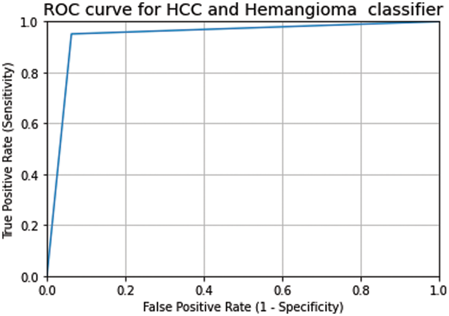
Figure 6: The ROC curve and AUC score of the classification of testing data on the ensemble of the best three models (AUC = 0.94)

6  Discussion

The benign liver tumor composed of blood-filled cavities clusters known as Hepatic hemangiomas [39]. In Hepatic hemangiomas, the clusters of blood-filled cavities are surrounded by endothelial cells supplied by the liver artery. Most Hepatic hemangiomas are asymptomatic and often accidentally found in imaging studies of unrelated diseases. Capillary hemangiomas are a kind of hemangiomas with size ranges between a few mm and three cm, and their size does not increase over time. Therefore, they do not cause future symptoms. Medium and small-size hemangiomas usually require regular follow-up but do not require active treatment. Occasional reports stated that big-size (around 10 cm and can reach 20+ cm) hemangiomas could develop complications and symptoms that need surgical interventions or other types of treatment. A careful diagnosis is required to differentiate between Hepatic hemangiomas and other liver diseases; also co-occurring diagnosis is required. There are many types of imaging techniques for diagnosing Hepatic hemangiomas. These imaging techniques include contrast-enhanced CT scan, ultrasound, contrast-enhanced ultrasound, and MRI. Among these techniques, ultrasound is recommended especially for patients with liver cancer-related cirrhosis and for diagnosing liver hemangioma, and they are showing promising screening results. Besides, ultrasounds are widely available, can be reproduced, and do not have irradiation effects. Therefore, they are considered the first diagnostic step for Hepatic hemangiomas.

Routine ultrasound screening is widely available now. Therefore, Hepatic hemangiomas are now more frequently detected than before. Pathologically, many endothelial-lined vascular spaces compose hemangiomas. A fibrous septum separates these endothelial-lined vascular spaces. The overall size of these vascular spaces can vary. Now it is essential to distinguish between hemangiomas and other hepatic tumors, and this is achieved in 95% of the cases without requiring further investigation using contrast-enhanced ultrasound. However, some uncertainty may occur if there is a typical enhanced pattern. The percentage of the precise primary diagnosis (before histologic examination and surgery) can be increased if practitioners are familiar with the appearance of Hepatic hemangiomas on ultrasound or contrast-enhanced ultrasound. Gray scale ultrasound show hemangiomas as well-defined lesions and further investigation will be required if the feature is atypical in conventional ultrasound. For focal liver lesions characterization, contrast-enhanced ultrasound is found to be reliable and particular. Operators with high skills and adequate equipment are required to detect small nodules in the cirrhotic liver. Such operators or equipment may only be available sometimes. Therefore, computational methods trained in ultrasound images will be highly beneficial. The approach proposed in this study shows a detection accuracy of 94% on ultrasound images. Based on the properties of the contrast-enhanced ultrasound that we discussed in this section, our approach can even show higher accuracy.

The main limitations of ultrasound are that it depends heavily on operators and patients [39]. They show the Hepatic hemangiomas as hyperechoic homogenous nodules with clear margins with posterior acoustic enhancement. Also, in ultrasound, the Hepatic hemangiomas usually do not change in size in the follow-up exams when comparing the current and previous scans. Hepatic hemangiomas’ histology explains Hyperechoic ultrasound patterns. Hyper echogenicity is the result of a large number of interfaces between the Hepatic hemangiomas-composite endothelial sinuses and their blood. In the case of larger lesions, the images are classified as inhomogeneous with hypoechoic and hyperechoic, and that is due to possible necrosis, hemorrhage, or connective tissue fibrosis. The lesions with this pattern are considered Hepatic atypical hemangiomas, showing no Doppler signals in the Doppler ultrasound.

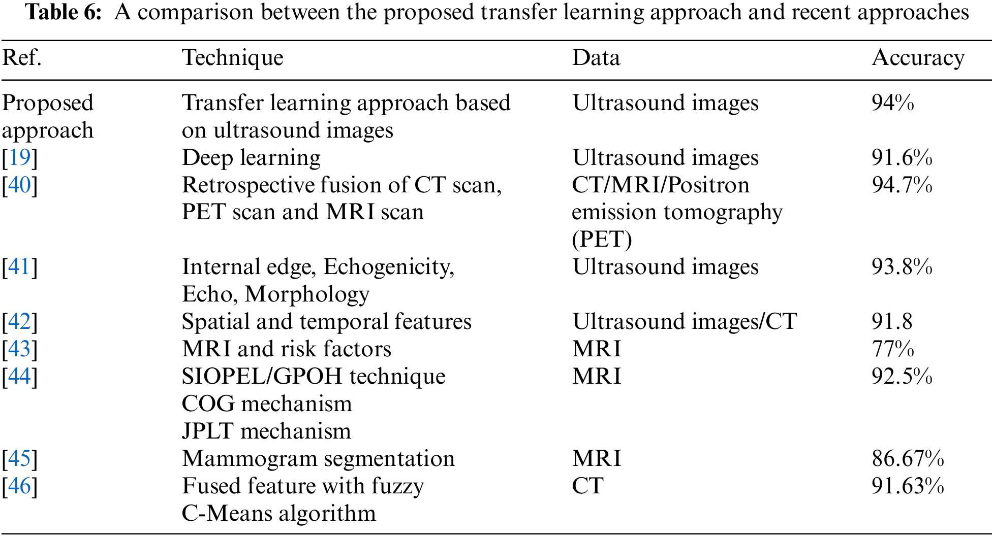
Table 6 shows a comparison between our proposed approach and other existing methods for liver cancer classification. Our method achieves the highest classification accuracy among the ultrasound image methods. Although the authors of [40] achieved a classification accuracy that is slightly higher than our methods, they used MRI images that have side effects and can be obtained at a high cost. Our proposed method can avoid side effects and reduce the cost of obtaining images. The authors of [19] achieved an accuracy of 91.6% using deep learning on ultrasound images. They first used ResNet50 Neural Network to resize the images of size 240 × 345 to 8 × 11. Then they used an attention block to detect image anomalies, and their final prediction results were obtained using logistic regression. The authors of [41] and [42] also utilized ultrasound images and obtained currencies of 93.8% and 91.8%, respectively. The authors of [41] performed feature extraction, enhancement, utilized support vector machines, and artificial neural networks as computer-aided diagnostics. The authors of [42] obtained features in three phases and performed classification in two stages, and they used linear and nonlinear SVMs with radial basis functions in their method. The authors of [43–45] used MRI images in their classification methods, while the authors of [46] used CT scan images.

7  Conclusion

This paper proposed an ensemble method based on transfer deep learning. The dataset used is obtained from three different sources. We experimented in 5 stages using 14 different on-the-shelf models. In the first stage, we applied the on-the-shelf models in the original dataset to create base-line-models. In the second stage, we augmented the dataset and then retrained the baseline models on the augmented data. In the third stage, we selected the top 3 models with the highest performance in stage two, and we fine-tuned the features extraction part of these models to select the best-retrained point for each model. In stage 4, we tuned the classification layer of the best top three performing models by adding different dense layers after the feature extraction part of each model and then measuring the validation accuracy to select the best classification configurations. In stage 5, we applied the ensemble approach to the best three models obtained in stage 4 using the average voting process. Our proposed approach achieved a test accuracy, precision, recall, and F1-measure score of 95%. This paper deals with primary liver cancer (HCC), the most common primary hepatic malignant tumor, and Hemangioma, the second most common benign hepatic lesion. HCC refers to the development of cancer in the liver’s tissue. Other liver cancers are caused by the spread of cancer in the liver from other body parts. These kinds of cancers are known as metastatic liver cancer, and doctors refer to these cancers as the same type of primary cancer, such as melanoma, colorectal, and gastrointestinal cancers. In addition, another kind of liver cancer that affects the ducts that drain bile from the liver is called Cholangiocarcinoma. In future works, we intend to develop a computational method based on deep learning to classify the aforementioned types of cancers.

Funding Statement: This work was funded by the Deanship of Scientific Research at Jouf University under Grant No. (DSR-2022-RG-0104).

Conflicts of Interest: The authors declare that they have no conflicts of interest to report regarding the present study.

References

1. J. Hepatol, “EASL clinical practice guidelines: Management of hepatocellular carcinoma,” National Library of Medicine, European Association for the Study of the Liver, vol. 69, no. 1, pp. 182–236, 2018. [Google Scholar]

2. J. Zhou, H. Sun, Z. Wang, W. Cong, J. Wang et al., “Guidelines for diagnosis and treatment of primary liver cancer in China,” National Library of Medicine, European Association for the Study of the Liver,vol. 7, no. 3, pp. 235–260, 2018. [Google Scholar]

3. J. Marrero, L. Kulik, C. Sirlin, A. Zhu, R. Finn et al., “Diagnosis, staging, and management of hepatocellular carcinoma,” Practice Guidance by the American Association for the Study of Liver Diseases, Hepatology, vol. 68, no. 2, pp. 723–750, 2018. [Google Scholar]

4. I. Kononenk, “Machine learning for medical diagnosis: History, state of the art and perspective,” Artificial Intelligence in Medicine, Elsevier, vol. 23, no. 1, pp. 89–109, 2001. [Google Scholar] [PubMed]

5. A. Krizhevsky, I. Sutskever and G. Hinton, “ImageNet classification with deep convolutional neural networks,” Advances in Neural Information Processing Systems, vol. 25, no. 2, pp. 1097–1105, 2012. [Google Scholar]

6. K. Simonyan and A. Zisserman, “Very deep convolutional networks for large-scale image recognition,” Computer Vision and Pattern Recognition, arXiv: 1409.1556, 2015. [Google Scholar]

7. M. Elbashir, M. Ezz, M. Mohammed and S. Saloum, “Lightweight convolutional neural network for breast cancer classification using RNA-seq gene expression data,” IEEE Access, vol. 7, pp. 185338–185348, 2019. [Google Scholar]

8. H. Jiang, R. Zheng, D. Yi and D. Zhao, “A novel multi-instance learning approach for liver cancer recognition on abdominal CT images based on CPSO-SVM and IO,” Computational and Mathematical Methods in Medicine, vol. 2013, pp. 1–11, 2013. [Google Scholar]

9. R. Rajagopal and P. Subbaiah, “Computer aided detection of liver tumor using SVM classifier,” International Journal of Advanced Research in Electrical, Electronics and Instrumentation Engineering, vol. 3, no. 6, pp. 10170–10177, 2014. [Google Scholar]

10. S. Naeem, A. Ali, S. Qadri, W. Mashwani, N. Tairan et al., “Machine-learning based hybrid-feature analysis for liver cancer classification using fused (MR and CT) images,” Applied Sciences, MDPI, vol. 10, no. 9, pp. 1–22, 2020. [Google Scholar]

11. M. Hussain, N. Saher and S. Qadri, “Computer vision approach for liver tumor classification using CT dataset,” Applied Artificial Intelligence, vol. 36, no. 1, pp. 1–24, 2022. [Google Scholar]

12. V. Hemalatha and C. Sundar, “Automatic liver cancer detection in abdominal liver images using soft optimization techniques,” Journal of Ambient Intelligence and Humanized Computing, vol. 12, no. 5, pp. 4765–4774, 2021. [Google Scholar]

13. F. Alam, S. Alrajhi, M. Nassar and A. Afify, “Modeling liver cancer and leukemia data using arcsine-Gaussian distribution,” Computers, Materials & Continua (CMC), vol. 67, no. 2, pp. 2185–2202, 2021. [Google Scholar]

14. M. Ragab and J. Alyami, “Stacked gated recurrent unit classifier with CT images for liver cancer classification,” Computer Systems Science & Engineering (CSSE), vol. 44, no. 3, pp. 2309–2322, 2023. [Google Scholar]

15. L. Meng, Y. Tian and S. Bu, “Liver tumor segmentation based on 3D convolutional neural network with dual scale,” Journal of Applied Clinical Medical Physics, vol. 21, no. 1, pp. 144–157, 2020. [Google Scholar] [PubMed]

16. A. Kaur, A. Chauhan and A. Aggarwal, “An automated slice sorting technique for multi-slice computed tomography liver cancer images using convolutional network,” Expert Systems with Applications, Elsevier, vol. 186, pp. 1–11, 2021. [Google Scholar]

17. S. Almotairi, G. Kareem, M. Aouf, B. Almutairi and M. Salem, “Liver tumor segmentation in CT scans using modified SegNet,” Sensors, MDPI, vol. 20, no. 5, pp. 1–13, 2020. [Google Scholar]

18. M. Hassan, S. Ali, M. Sanaullah, K. Shahzad, S. Mushtaq et al., “Drug response prediction of liver cancer cell line using deep learning,” Computers, Materials & Continua (CMC), vol. 70, no. 2, pp. 2743–2760, 2022. [Google Scholar]

19. B. Schmauch, P. Herent, P. Jehanno, O. Dehaene, C. Saillard et al., “Diagnosis of focal liver lesions from ultrasound using deep learning,” National Library of Medicine, European Association for the Study of the Liver, vol. 100, no. 4, pp. 227–233, 2019. [Google Scholar]

20. H. Park, J. Park, D. Kim, S. Ahn, C. Chon et al., “Characterization of focal liver masses using acoustic radiation force impulse elastography,” National Library of Medicine, European Association for the Study of the Liver, vol. 19, no. 2, pp. 219–226, 2013. [Google Scholar]

21. H. Choi, I. Banerjee, H. Sagreiya, A. Kamaya, D. Rubin et al., “Machine learning for rapid assessment of outcomes of an ultrasound screening and surveillance program in patients at risk for hepatocellular carcinoma,” in Scientific Assembly and Annual Meeting of Radiological Society of North America, Chicago, USA, pp. 1–15, 2018. [Google Scholar]

22. X. Liu, J. Song, S. Wang, J. Zhao and Y. Chen, “Learning to diagnose cirrhosis with liver capsule guided ultrasound image classification,” Sensors, MDPI, vol. 17, no. 1, pp. 1–17, 2017. [Google Scholar]

23. P. Raj, K. Kalimuthu, S. Gauni and C. Manimegalai, “Extended speckle reduction anisotropic diffusion filter to despeckle ultrasound images,” Intelligent Automation & Soft Computing (IASC), vol. 34, no. 2, pp. 1187–1196, 2022. [Google Scholar]

24. A. Abdalla, M. Awad, O. AlZoubi and L. Al-Samrraie, “Automatic segmentation and detection system for varicocele using ultrasound images,” Computers, Materials & Continua (CMC), vol. 72, no. 1, pp. 797–814, 2022. [Google Scholar]

25. G. Karthiha and S. Allwin, “Speckle noise suppression in ultrasound images using modular neural networks,” Intelligent Automation & Soft Computing (IASC), vol. 35, no. 2, pp. 1753–1765, 2023. [Google Scholar]

26. M. Lv, G. Zhou, M. He, A. Chen, W. Zhang et al., “Maize leaf disease identification based on feature enhancement and DMS-robust alexnet,” IEEE Access, vol. 8, pp. 57952–57966, 2020. [Google Scholar]

27. X. Qiang, G. Zhao, A. Chen, X. Zhang and W. Zhang, “Forest fire smoke detection under complex backgrounds using TRPCA and TSVB,” International Journal of Wildland Fire, vol. 30, no. 5, pp. 329–350, 2021. [Google Scholar]

28. Z. Wang, B. Du and Y. Guo, “Domain adaptation with neural embedding matching,” IEEE Transactions on Neural Networks and Learning Systems, vol. 31, no. 7, pp. 1–11, 2019. [Google Scholar]

29. H. Kim, A. Cosa-Linan, N. Santhanam, M. Jannesari and M. Maros, “Transfer learning for medical image classification: A literature review,” National Library of Medicine, European Association for the Study of the Liver, vol. 22, no. 1, pp. 1–13, 2022. [Google Scholar]

30. https://www.sonoskills.com/en-en/resources/ultrasound-cases/ [Last Access: 03-11-2022]. [Google Scholar]

31. https://sonographie.org/en/ [Last Access: 02-11-2022]. [Google Scholar]

32. https://radiopaedia.org/ [Last Access: 03-11-2022]. [Google Scholar]

33. C. Lee, P. Gallagher and Z. Tu, “Generalizing pooling functions in convolutional neural networks: Mixed gated and tree,” IEEE Transactions on Pattern Recognition, vol. 40, pp. 863–875, 2018. [Google Scholar]

34. L. Alzubaidi, M. Al-Amidie, A. Al-Asadi, A. Humaidi, O. Al-Shamma et al., “Novel transfer learning approach for medical imaging with limited labeled data,” Cancers, vol. 13, no. 7, pp. 1–22, 2021. [Google Scholar]

35. S. Tajbakhsh, S. Gurudu, R. Hurst, C. Kendall, M. Gotway et al., “Convolutional neural networks for medical image analysis: Full training or fine tuning,” IEEE Transactions on Medical Imaging, vol. 35, no. 5, pp. 1299–1312, 2016. [Google Scholar] [PubMed]

36. V. Jayaram, M. Alamgir, Y. Altun, B. Schölkopf and M. Grosse-Wentrup, “Transfer learning in brain-computer interfaces,” IEEE Computational Intelligence Magazine, vol. 11, no. 1, pp. 20–31, 2015. [Google Scholar]

37. D. Flores, P. Velázquez, H. Hernández, A. Domínguez, M. Chapa et al., “A safely resected, very large hepatic hemangioma,” National Library of Medicine, European Association for the Study of the Liver, vol. 5, pp. 1–2, 2018. [Google Scholar]

38. M. Ezz, A. Mostafa and A. Elshenawy, “Challenge-response emotion authentication algorithm using modified horizontal deep learning,” Intelligent Automation & Soft Computing (IASC), vol. 35, no. 3, pp. 3659–3675, 2023. [Google Scholar]

39. N. Bouknani, A. Rami, M. Kassimi and M. Mahi, “Exophytic hepatic hemangioma: A case report,” Radiology Case Report, Elsevier, vol. 17, no. 9, pp. 3367–3369, 2022. [Google Scholar]

40. A. Parsai, M. Miquel, H. Jan, A. Kastler, T. Szyszko et al., “Improving liver lesion characterization using retrospective fusion of FDG PET/CT and MRI,” Molecular Imaging and Nuclear Medicine, vol. 55, pp. 23–28, 2019. [Google Scholar]

41. N. Ta, Y. Kono, M. Eghtedari, T. Oh, M. Robbin et al., “Focal liver lesions: Computer-aided diagnosis by using contrast-enhanced us cine recordings,” Radiology, vol. 3, pp. 1062–1071, 2018. [Google Scholar]

42. S. Kondo, K. Takagi, M. Nishida, T. Iwai, Y. Kudo et al., “Computer-aided diagnosis of focal liver lesions using contrast-enhanced ultrasonography with perflubutane microbubbles,” IEEE Transaction on Medical Imaging, vol. 7, pp. 1427–1437, 2017. [Google Scholar]

43. J. Mariëlle, H. Kuijf, W. Veldhuis, F. Wessels, M. Viergever et al., “Automatic classification of focal liver lesions based on MRI and risk factors,” PLoS ONE, vol. 14, no. 5, pp. 1–13, 2019. [Google Scholar]

44. J. Oliva, H. Lee, N. Spolaôr, C. Coy and F. Wu, “Prototype system for feature extraction, classification and study of medical images,” Expert Systems with Applications, vol. 63, pp. 267–283, 2016. [Google Scholar]

45. R. Boss, S. Chandra, K. Thangavel and D. Daniel, “Mammogram image segmentation using fuzzy clustering,” in Proc. of the Int. Conf. on Pattern Recognition, Informatics and Medical Engineering, Salem, India, pp. 290–295, 2012. [Google Scholar]

46. W. Wu, S. Wu, Z. Zhou, R. Zhang and Y. Zhang, “3D liver tumor segmentation in CT images using improved fuzzy C-means and graph cuts,” BioMed Research International, vol. 5207685, pp. 1–12, 2017. [Google Scholar]