Traffic Sign Detection with Low Complexity for Intelligent Vehicles Based on Hybrid Features

1  Introduction

Detecting traffic signs is considered a significant field of research in image processing, computer vision, pattern recognition, and machine learning. Huge research is continuously going on for decades because of its applications in advanced driver assistance systems (ADAS) [1], autonomous driving [2,3], and traffic signs maintenance and inventory management systems using robots [4,5]. A traffic sign detector is used to help drivers while driving by giving warnings and guidance so that a probable accident can be avoided. Similarly, manually checking the existence and state of traffic signs is mind-numbing work [6] that a sign detector can easily handle; robots can be activated automatically using road and traffic signs which depend on the fact of recognizing and identifying these landmarks.

The number of vehicles on the road is increasing day by day, which also causes a rise in the ratio of accidents [7]. The primary reasons for such accidents are the absence of traffic signs, alteration of traffic signs, occlusion of a traffic sign, tiredness or absence of the mind of drivers, and much more. The better flow of traffic, vehicle, and pedestrian safety becomes easy with the help of an effective traffic sign detector.

Traffic signs may differ in color or shape in different countries and even maybe categorized differently. However, to make unanimous traffic sign classes, an effort was made at the Vienna Convention in the late 60s [8]. In that convention, signs were classified into different classes that are now used in many countries. Many countries are implementing it, which is helpful while developing an approach for traffic sign detection (TSD).

Many issues exist in TSD, as shown in Fig. 1, which have been given a focus for decades but still need more effort. These systems have hurdles and troubles faced in object recognition in the natural environment. Some of the reasons for such difficulties are a variety of weather conditions, variation of light geometry, partial or complete occlusion, motion artifacts, illumination, presence of a similar object, etc. [9].

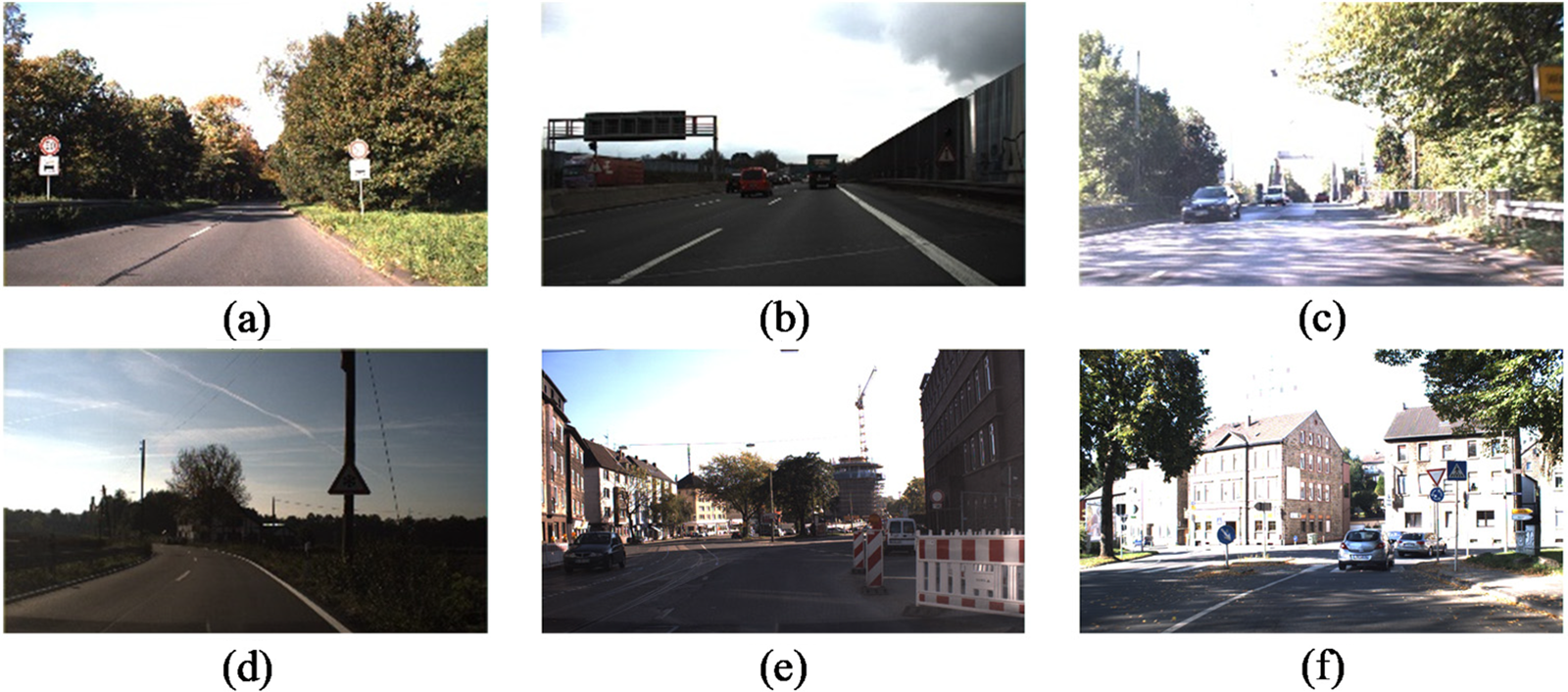
Figure 1: Factors affecting TSD: (a) illumination; (b) bad weather; (c) variation of light geometry; (d) darkness; (e) similar objects; (f) cluttered background

2  Contributions and Motivation

The proposed methodology focuses on detecting traffic signs in images in the dark, far away, partially occluded, and affected by the lighting or the presence of similar objects, which is a complicated and cumbersome task. Traffic signs correct detection is a significant task in all applications related to traffic signs, as TSD is the first stage and all other stages depend on its results. To make this task easier, a modified version of the red-green component enhancement formula is used before segmentation. Furthermore, a fusion of features from existing features of color and texture is used to detect traffic signs, reducing false positives (FP) and false negatives (FN). The contribution of our work is:

•   Modifying an existing enhancement formula

•   Creating new fused feature sets on channels of different color models

•   Attaining a 98.5% accuracy with quadratic SVM with reduced FP and FN

3  Literature Review

Primarily, a restricted sort of research was going on TSD; that is, a single image was used, and only a single class of traffic signs were researched, usually circular signs [10]. For problem simplification, some assumptions were also used [11]. However, the field is becoming vast over time, and limitations are starting to be reduced. Nowadays, researchers move on from one single image to multiple images and videos and from a single class of traffic signs to multiple classes [12].

TSD plays a crucial role in its relevant applications as its primary function is to locate traffic signs in images that may be further provided to other systems like traffic sign recognition (TSR) system, which are directly affected by its performance, better detection of signs by TSD leads to a better and efficient performance by other relevant systems [13]. Thus, TSD is a costly and crucial system because it is troublesome to find out a region of interest, i.e., a traffic sign, from the whole image captured by the camera. Image enhancement, image denoising, region of interest (ROI) extraction, ROI refinement, boundary detection, and segmentation are different processes that may be performed in TSD to obtain blobs and potential candidates. Multiple TSD systems are categorized as shape, color, or hybrid, which combines color and shape-based approaches [14]. Traffic signs’ color and shape are significant properties that distinguish them from other environmental objects [15]. Color information is considered the most significant property of traffic signs as they are of a particular color that quickly makes them distinguishable from other objects. Hence, researchers are more focused on using this characteristic while devising new segmentation approaches. Typically RGB [16–19] is light-sensitive but natural, so it needs less computation. Red, Green, and Blue Normalized (RGBN) [20], a variation of RGB that decreases the effect of illumination, and HSV [21] are near to human eye perception and less affected by illumination, but computational cost is high and is used mainly by researchers. Other color spaces like Commission on Illumination Lab (CIELab) [22], luminance with chromaticity values of the color image named LUV [23], and YCbCr [24,25] are also used by some researchers. In YCbCr, Y denotes the luma component whereas Cb and Cr represent blue and red difference chroma components respectively.

After segmentation and ROI extraction based on color or shape, different feature descriptors are used by researchers for further proceedings, such as Histogram of Oriented Gradients (HOG) [26–29], Local Self-Similarity (LSS) [21], Local Binary Pattern (LBP) [30], Scale-invariant feature transform (SIFT) [31], Speeded-Up Robust Feature (SURF) [32,33], Haar-like wavelet [34,35], Gabor filter and its bank [36,37], color moments [38,39], color histogram [40], Gray Level Co-occurrence Matrix (GLCM)/Haralick features [41,42], yet mostly HOG and its variants are given preference by the researchers like Pyramid Histogram of Oriented Gradient (PHOG) [43–45]. Huang et al. [43] proposed HOG variant (HOGv), an improved version of HOG, that used both signed and unsigned orientation to get more salient information about signs and used principal component analysis (PCA) to reduce every cell normalized histogram dimensions so that redundant information can be avoided. Kassani et al. [44] developed Soft HOG (SHOG) descriptor, a HOG variant that is compact and robust and discovers the optimum positions of cell histogram by manipulating symmetrical features of traffic signs.

Although redundant features with huge dimensions by the HOG descriptor may drop the efficiency of TSD, SIFT descriptors produce features with inconsistent dimensions due to sparse representation of various key points that may also decay the performance [30,46]. In the same way, every feature descriptor has some limitations, even though color moments and haarlick features are simple, less complex, and less used in TSD.

Classification is followed by feature extraction, in which ROIs are classified in traffic and non-traffic regions. The classifiers that are primarily used for this purpose are SVM [28,47,48], K-Nearest Neighbors (KNN) [49,50], Adaboost [51,52], Neural Networks (NNs) [17,53,54], etc. New classification models are used for extracting and selecting prudent features, minimizing the problem of overfitting and quicker results. Some researchers have proposed new frameworks for classification [16,44,55], especially deep learning [56–59]. Gudigar et al. [60] used Linear Discriminant Analysis (LDA) for the detection of traffic signs by extracting GIST features that are based on gradient information (scales and orientations). Different researchers mostly use NNs for both the classification and detection of traffic signs; such as Zhu et al. [61] used Fully Convolutional Networks (FCN), and Convolutional Neural Networks (CNN), and Kumar et al. [62] used Artificial Neural Networks (ANN). Similarly, Liu et al. [54] and Wan et al. [63] used You Only Look Once version 3 (YOLOv3), Liu et al. [64] used Scale Aware and Domain Adaptive network (SADANet), and Ayachi et al. [65] proposed a complete dataset with deep learning techniques for detection.

Although deep learning is now the focus of research, it has limitations in the dataset. Instead, other TSD approaches do not require vast amounts of data as deep learning-based methods required like in TSingNet [66] three datasets used for training an attention-driven bilateral feature pyramid network to detect small or occluded traffic signs in wild. In such approaches, color-based approaches are given more focus than colorless approaches as colorless approaches are more complex and time-consuming, whereas color-based approaches are time and computationally cost-efficient. Some researchers, although, used hybrid approaches as well to combine the benefits of both. They then later use machine learning and neural networks to get better results at the detection stage.

4  Proposed Methodology

In the proposed methodology, different steps are used to achieve the goal of detection, like denoising, color channel enhancement, segmentation, feature extraction, feature ensemble, and classification. Further, experiments with those features are performed to find the optimal solution. The proposed methodology is depicted in Fig. 2, which takes an input image and, after the denoising process, passes for segmentation followed by feature extractions. Then finally passed to SVM for classifying it into traffic and non-traffic signs; only traffic signs are depicted in the output image at the end.

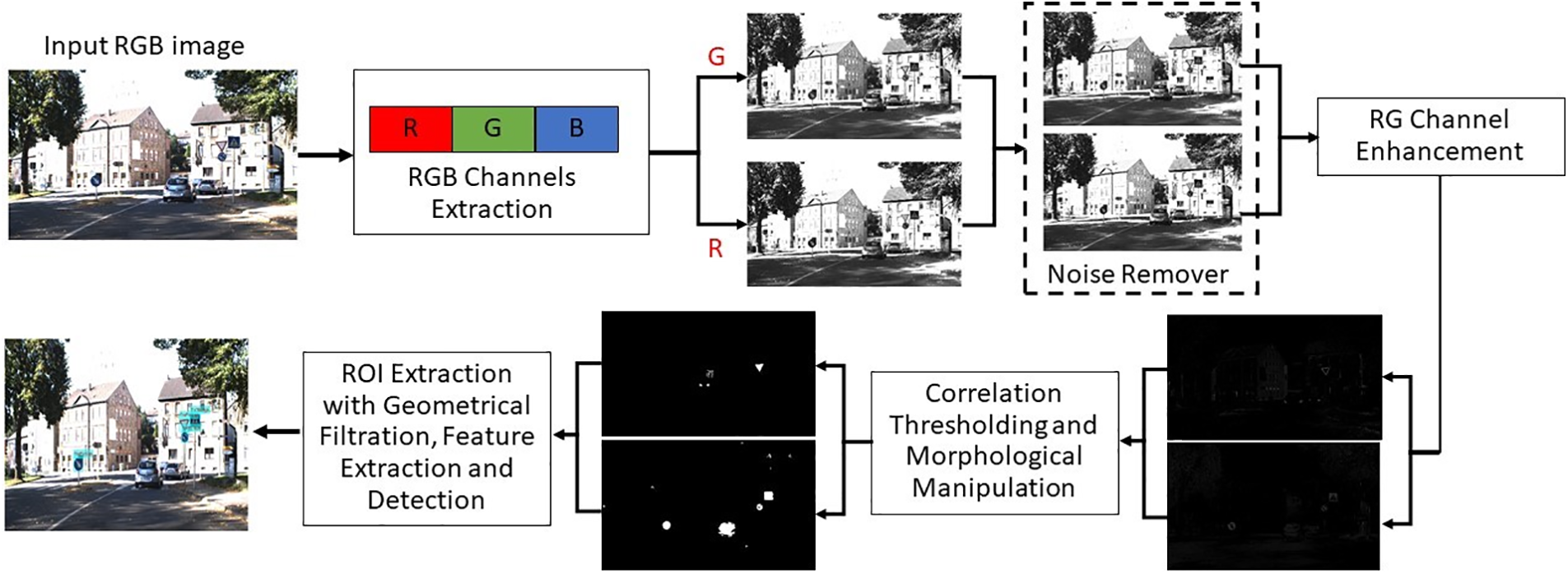
Figure 2: The proposed TSD approach

For better understanding and readability, Table 1 summarizes some important notations used in this paper. These notations are also explained in detail to make the grasp of the proposed methodology easy, with their relevant equations.

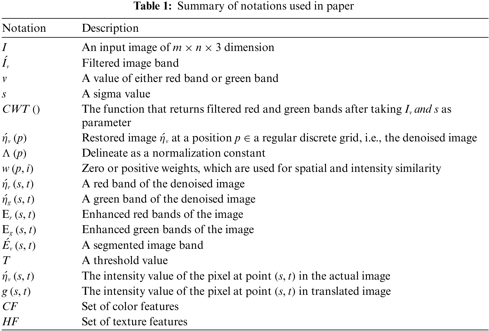
At first, a digital image from the dataset is taken on which sigma is estimated to determine the noise level that is supposed to be applied on the split red and green channel after passing through the dual-tree complex wavelet transform (CWT) [67] module. This module is designed to eliminate the image’s low frequencies and pass high frequencies.

Let I be an input image of m×n×3 dimension that splits into red and green bands Ir and Ig. Image of m×n dimension that passes as an argument to CWT function that returns filtered red and green band Ir´ and Ig´ respectively, i.e.,

Iv´=CWT(Iv,s).

Here Iv´ is used to represent a filtered image band and Iv denote the original image band, where v represents a green and red channel. The estimated sigma value s of the original image I is also passed in this filtration process.

After this step, a nonlinear averaging-based fast non-local mean filter is used to reduce the illumination effect. An image with repetitive or monotonous patterns can be denoised by a fast NL-means approach [68]. The weighted mean of pixels is used to reduce noise in this approach.

Let a regular discrete grid α with dimension d and cardinality |α| be used to define an image. If the noisy image Iv´ then the restored image η´v at a position, p∈α can be described as in Eq. (1):

η´v(p)=1Λ(p)∑i∈N(p)w(p,i)Iv´(i),(1)

where Λ(p) is delineated as a normalization constant that can be written as in Eq. (2):

Λ(p)=∑i∈N(p)w(p,i),(2)

Moreover, N(p) is a searching window, a set of neighboring locations of p; and w(p,i) represents zero or positive weights which is used for spatial and intensity similarity measuring between two square regions located at positions q and i, and can be equated as in Eq. (3):

w(p,i)=gh(∑δϵdpGσ(δ)(Iv´(p+δ)−Iv´(i+δ))2),(3)

In Eq. (3) δ represents neighboring locations of discrete patching regions dp, Gσ is variance σ2 based Gaussian kernel, gh is a function that is continuous and non-increasing and uses h to control the filtering. The function gh may further be explained as

gh(0)=1

and

lim∞→+∞gh(y)=0

In general, a more extensive search window N(p) will enable greater robustness to be achieved; however, the added time consumption is a concern.

The returned denoised image is further enhanced, making red and blue traffic signs more visible. Traffic signs are mostly red and blue, but in our method, we ignored the blue plane and utilized the green plane instead due to much better results and efficiency. Red and green channel enhancement is performed to highlight the signs more than the rest of the objects. The enhancement can be defined as in Eqs. (4) and (5).

Er(s,t)=max(0,η´r(s,t)−η´g(s,t)η´r(s,t)+2η´g(s,t)).(4)

Eg(s,t)=max(0,η´g(s,t)−η´r(s,t)η´r(s,t)−2η´g(s,t)).(5)

Er(s,t) and Eg(s,t) represent enhanced red and green bands of the image, respectively; η´r(s,t) denote the red band and η´g(s,t) refer to a green band of the image in Eqs. (4) and (5). The enhanced channels are passed to a segmentation function S(Ev) which returns a segmented image Ev´(s,t) i.e., Ev´(s,t)=S(Ev). While segmentation, a threshold value is applied to the enhanced color band with area, eccentricity, and axis (major and minor) filters. Thresholding can be defined in Eq. (6) with a threshold value T:

Ev´(s,t)={0,Ev(s,t)≤T1,Ev(s,t)>T.(6)

In Eq. (7) T can be defined with the help of a constant value c, depending on the intensities in the images η´v(s,t) that is the intensity value of the pixel at point (s,t) in the actual image, and g(s,t) that is the intensity value of the pixel at point (s,t) in the translated image. η´v¯ and g¯ are mean calculated from intensity matrices η´v and g(s,t) respectively.

T=log10(∑s∑t[η´v(s+i,t+j)−η´v¯][g(s,t)−g¯]∑s∑t[η´v(s,t)−η´v¯]2∑s∑t[g(s,t)−g¯]2+1)c.(7)

After thresholding, the area of each region ai and both major axis aximajor and minor axis aximinor of each region in the threshold image is checked using Eq. (8), where k∈{major,minor}; i defines the number of regions in the image Ev´(s,t); μ and λ are the maximum and minimum areas, respectively, whereas a and b are the maximum and minimum axis for major and minor axis filtering, respectively, and p defines maximum eccentricity with q as the minimum one.

Ev´´(s,t)={0,μ<ai<λanda<axik<bandp<e<q1,λ≤ai≤μandb≤axik≤aandq≤e≤p.(8)

Area of each region i.e., ai is the total number of image pixels, i.e., N that make up a region and are defined as in Eq. (9).

ai=|i|=N.(9)

Major axis i.e., aximajor and minor axis i.e., axminor are calculated using Eqs. (10) and (11) with ϑ=112 and Δ=22.

aximajor=Δ.(∑x2N+ϑ)+(∑y2N+ϑ)+((∑x2N+ϑ)−(∑y2N+ϑ))2+4.(xyN)2(10)

aximinor=Δ.(∑x2N+ϑ)+(∑y2N+ϑ)−((∑x2N+ϑ)−(∑y2N+ϑ))2+4.(xyN)2(11)

In these equations, x and y are calculated, with the help of all pixels P in the region, using Eqs. (12) and (13).

x=Px−1|R|∑(u,v)∈Ru.(12)

y=Py1|R|∑(u,v)∈Rv.(13)

An eccentricity that is denoted by e defines how much a shape is elongated and can get through the following Eq. (14).

e=2.(aximajor2)2−(aximinor2)2aximajor.(14)

Figs. 3–5 depict the outcomes after segmentation and refinement of the input image that the proposed method obtained following all the steps described above. The segmented image may contain some other regions from the images due to color intensity, which are removed during extraction of the ROIs using some geometrical assumptions using height and width, which mostly filtered the non-traffic sign regions.

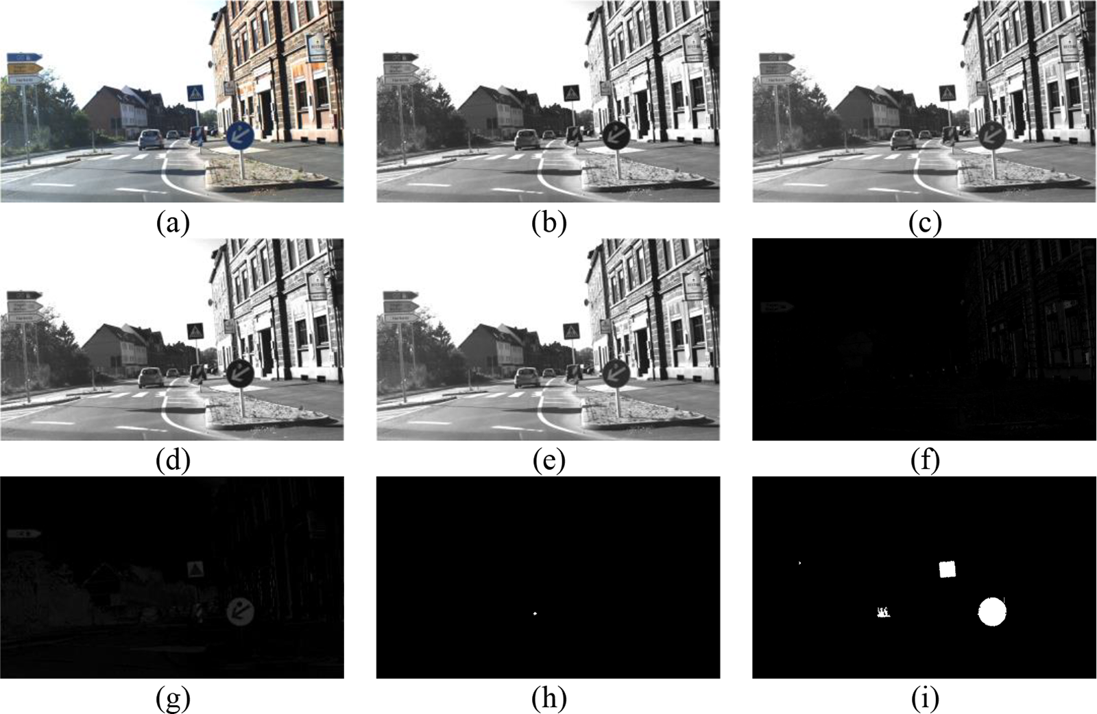
Figure 3: Segmentation process: (a) and (b) represent red and green channel respectively; (c) and (d) represent denoised red and green channel respectively; (f) and (g) represent enhanced red and green channel respectively; (h) and (i) represent thresholded and morphed red and green channel respectively

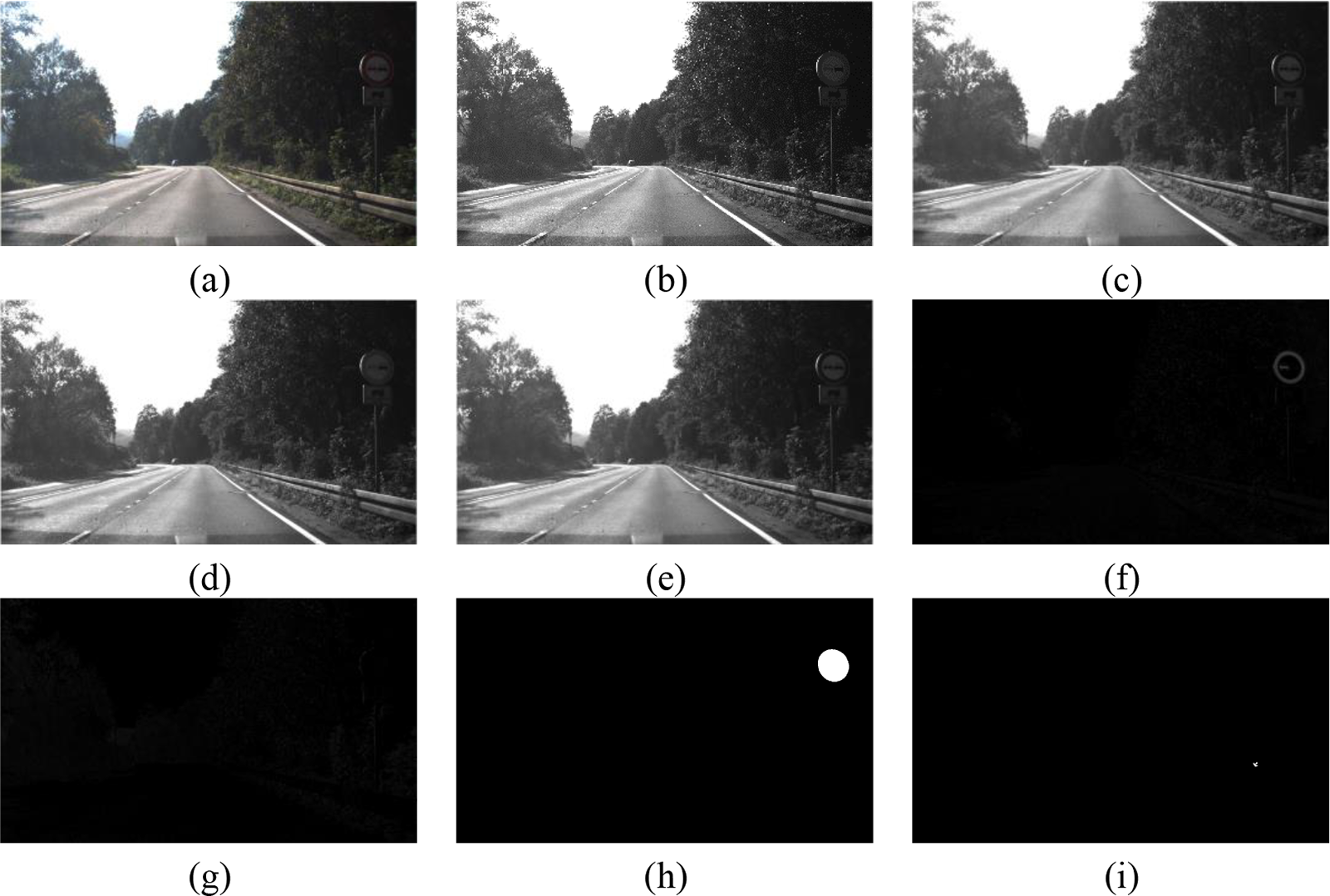
Figure 4: Segmentation process: (a) and (b) represent red and green channel respectively; (c) and (d) represent denoised red and green channel respectively; (f) and (g) represent enhanced red and green channel respectively; (h) and (i) represent thresholded and morphed red and green channel respectively

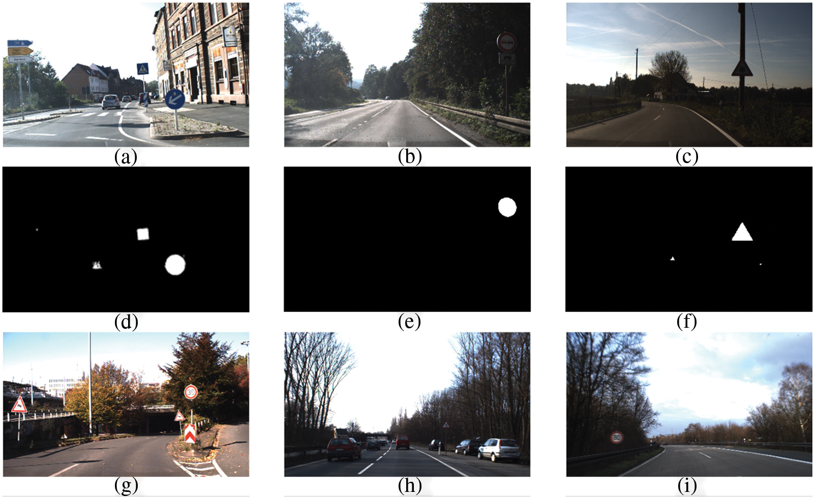
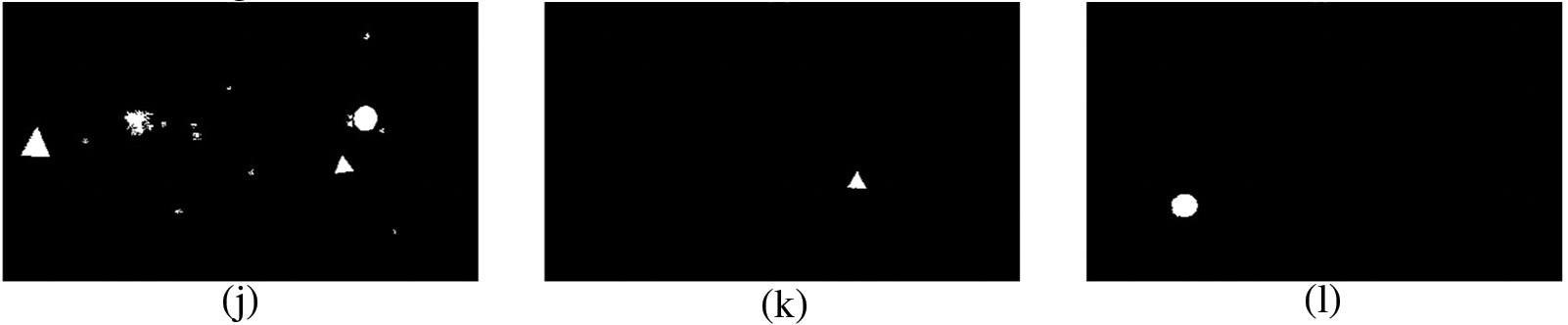
Figure 5: Segmentation results: (a–c) with (g–i) are original images, whereas (d–f) with (j–l) are respective segmented images

After ROI filtration during extraction, the remaining regions are used for feature extraction. Fig. 6 shows the process of fused feature calculation.

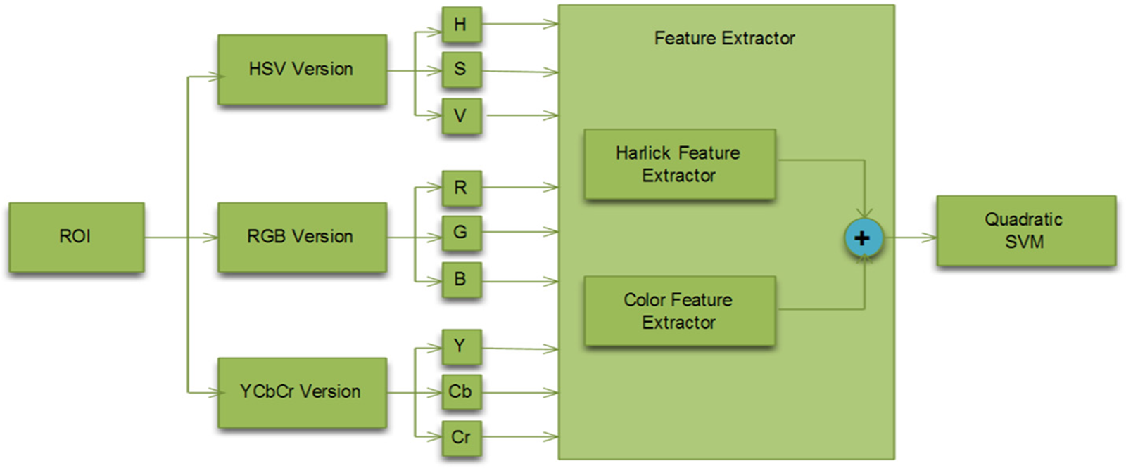
Figure 6: Feature extraction flow diagram

Now, only potential candidates that may be traffic signs will remain for which color feature vector and texture feature vector are calculated for each band of RGB, HSV, and YCbCr color space version of the image. Color features are invariant to the object’s size and orientation. In color features, mean (first-order), variance (second-order), range, and skewness (third-order) moments are calculated, which are more compact than other color features and demonstrated to be effective in representing the color distribution of images. Mean helps determine the image background, and variance describes the brightness, range, and skewness determining information about the shape of the color distribution. The feature vector for color contains 1305 moments, i.e., 145 moments for each band. Let the feature vector for color CF for N images with dimension N×1305 be defined as:

CF={CF1,CF2,CF3,…CFN}.

where CFi∈{1,2,3,…,N} consist of all four moments of each band of set colour={r,g,b,h,s,v,y,cb,cr} for every version of image I, i.e.,:

CFi=[μcolour,Scolour,Rcolour,Vcolour].

Here μcolour is the mean moment of the image Icolour with m×n total pixels, and calculated using the following Eq. (15):

μcolour=1mn∑s=0m−1∑t=0n−1Icolour(s,t).(15)

Scolour is the skewness moment of uth band, which is determined using µcolour that is the mean of the pixel at point (s,t) in Icolour, and σcolour that is, the standard deviation of the pixel at a specified point (s,t) in Icolour, described in the following formula:

Scolour=E(Icolour(x)−μcolour)3σcolour3.(16)

where σcolour is the standard deviation of color that is defined as:

σcolour=1mn(∑j=1N(Pij−Ei)3).(17)

and E(z) denotes the anticipated value of the quantity z. Rcolour is range moment that determines maximum and minimum intensities and Vcolour is the variance moment that is determined using µcolour is the mean of the pixel at point (s,t) in Icolour following formula:

Vcolour=1mn−1∑s=1N|Is−μcolour|2.(18)

In texture features, we calculated three Haralick texture features (correlation, homogeneity, and sum average) for better results and less computation time. Let feature vector for texture features HF for N images of N×27 dimension can be defined as:

HF={HF1,HF2,HF3,…HFN}.

where HFi∈{1,2,3,…,N} consist of all three features of each band of set colour={r,g,b,h,s,v,y,cb,cr} for every version of the image, i.e.,:

HFi=[Ccolour,Hcolour,SAcolour].

If I is an image, then the Correlation Ccolour of Icolour will be calculated with the help of mean μcolour and standard deviation σcolour of co-occurrence matrix (x, y) coordinates, and (s,t)th element of GLCM pcolour(s,t), as given in Eq. (19):

Ccolour=∑s∑t(st)pcolour(s,t)−μcolour(x)μcolour(y)σcolour(x)σcolour(y).(19)

Homogeneity H of the image I is calculated using Eq. (20) with the help of point (s,t) and probability at that point pcolour(s,t):

Hcolour=∑s∑t11+(s−t)2 pcolour(s,t)(20)

Sum Average SAcolour of image Icolour is calculated, using N the number of intensity levels, where px+y at point (x, y) is the probability of co-occurrence distribution, as in Eq. (21):

SAcolour=∑i=22Nspcolourx+y(s)(21)

Extracted features are fused together and passed to Quadratic SVM to detect traffic signs from filtered regions. Here, quadratic SVM is trained on the fusion of color and texture features and is selected after checking different classifiers. The said SVM provides better results, as shown in Fig. 7.

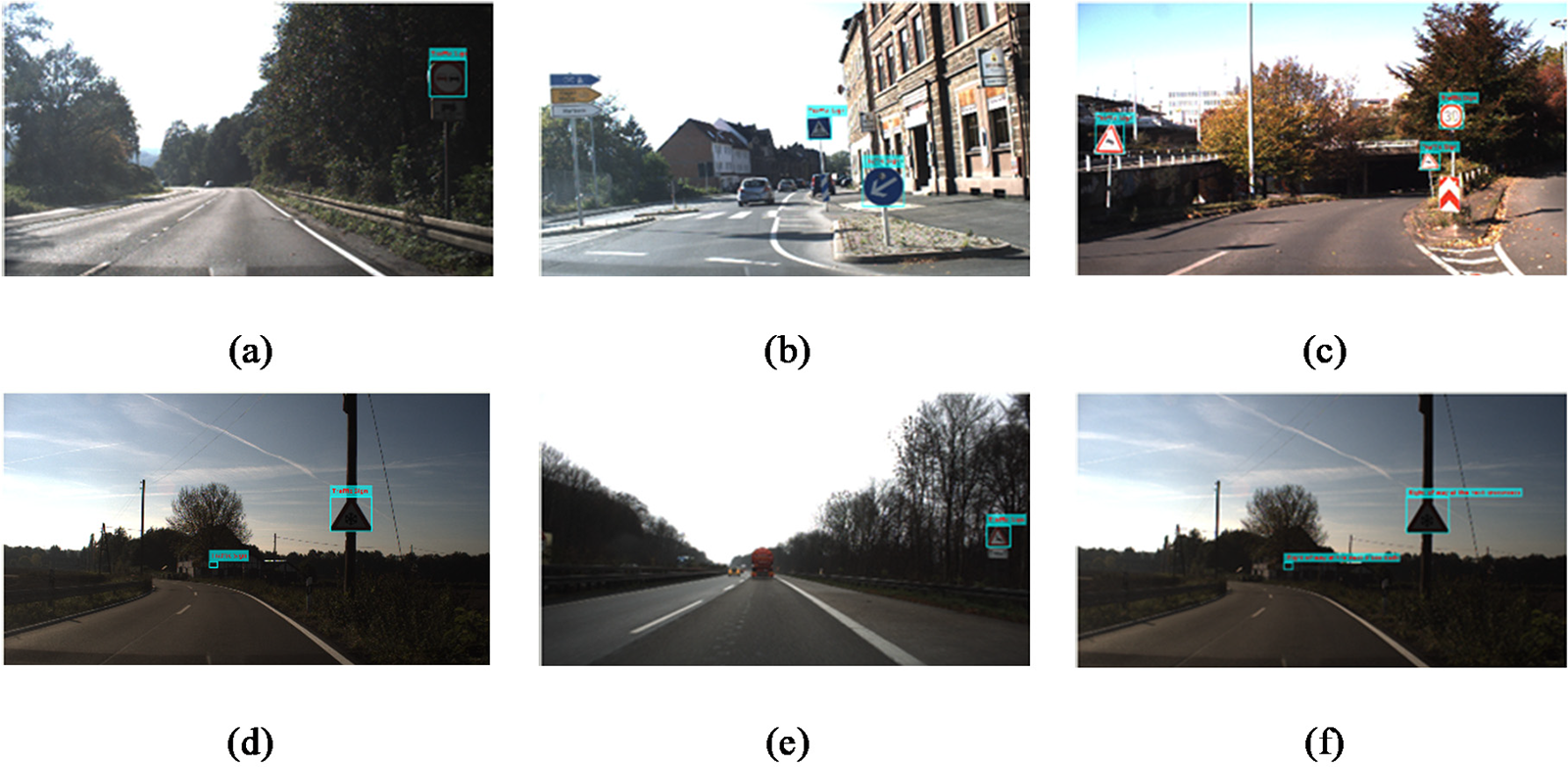
Figure 7: Detection and recognition results

5  Results and Discussion

Results are obtained using the German Traffic Sign Detection Benchmark (GTSDB) [69]. Fig. 8 presents a set of traffic signs in GTSDB. Images of 1360×800 pixels are taken from the dataset to test the approach containing at least one traffic sign. For the training roundabout, 1300 images are taken, and 700 images are used for testing. The complete experiment used 10-fold cross-validation. Color features and texture features are calculated for each image separately and then fused.

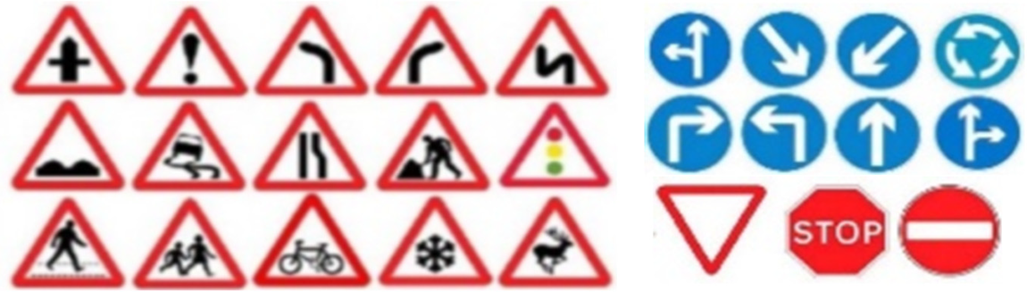
Figure 8: Traffic signs in GTSDB [69]

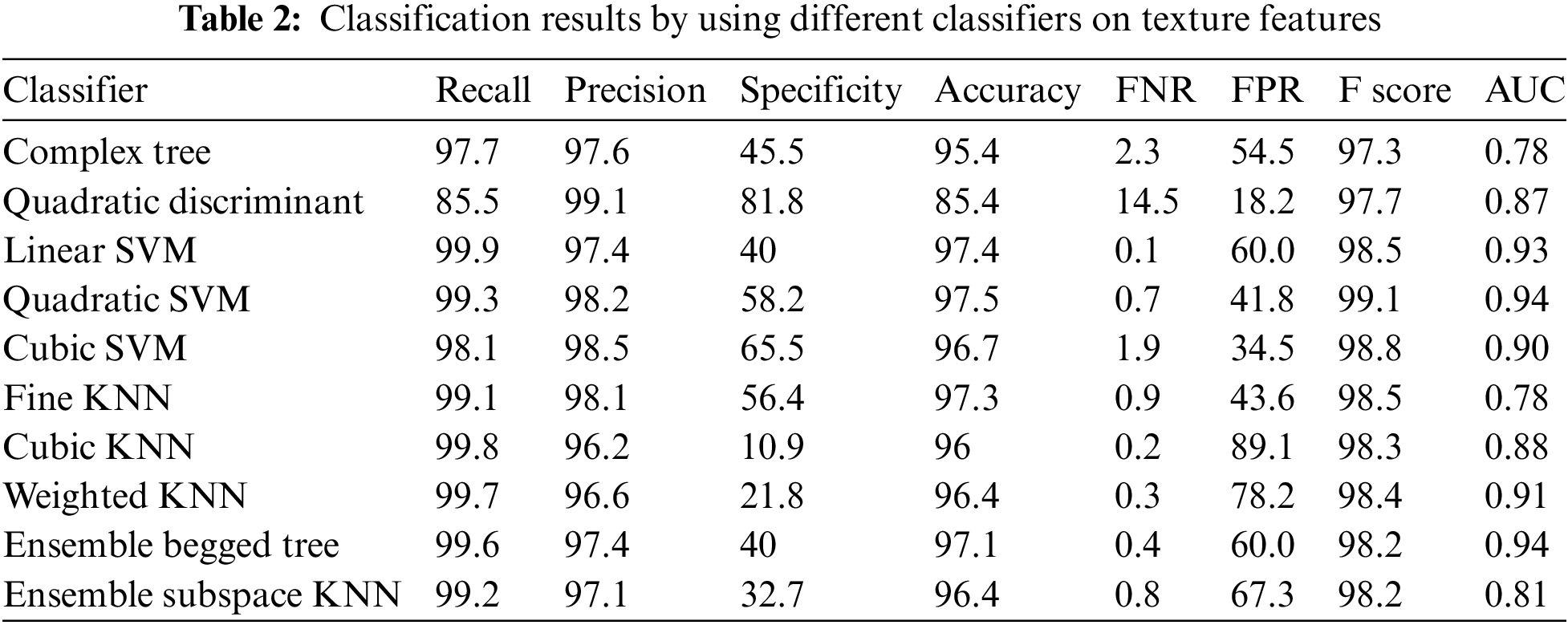
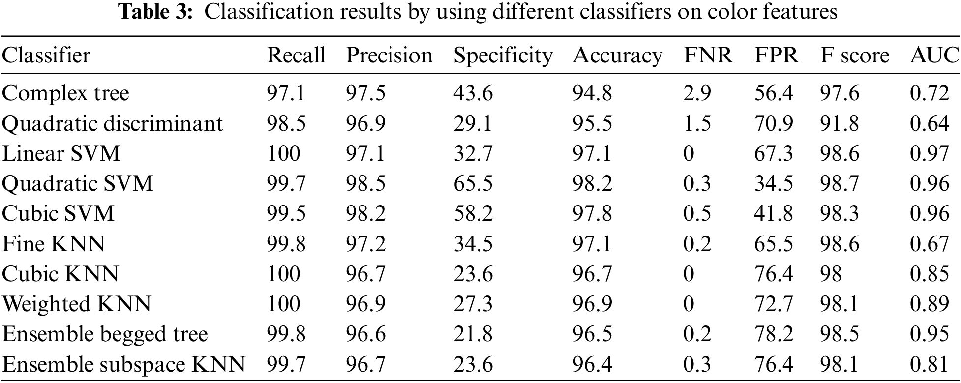
The classifier performance is evaluated based on the following evaluation parameter: Recall (TPR, i.e., true positive rate), Specificity (TNR, i.e., true negative rate), Accuracy, Precision, false negative rate (FNR), false positive rate (FPR), F-score and Area under Curve (AUC). Initially, results are taken separately on color and texture features and then on their fusion by combining them. The results show that the classifiers performed more accurately and showed reliable performance with reduced FPR on fused features, especially Quadratic SVM.

The following Tables 2 to 4 show the performance of different classifiers on the color, texture, and hybrid features, which illustrate entirely that Quadratic SVM performed better than the rest with high recall, accuracy, and low FPR on fused features. Table 2 illustrates the ten different classifiers’ performance on texture features, in which linear SVM has the highest recall rate with quite a high FPR, whereas quadratic SVM performs better as its detection rate is very close to linear SVM but relatively FPR is low. Similarly, the performance of the same ten selected classifiers for color features is shown in Table 3, which indicates that quadratic SVM again performed better than the rest and beat linear SVM similarly to texture features.

The final table for the same ten classifiers’ performance, Table 4, demonstrates that the quadratic SVM performed much better and more reliably when color and texture features are ensembled to form a fused feature vector than the remaining classifier. All these experiments help choose the SVM classifier in the proposed method.

SVM trained on color and texture features fusion is used while testing. SVM has performed with better and improved accuracy and reduced FPR as compared to the state-of-the-art algorithms and detects the traffic signs in little time in the test image. A comparison table, Table 5, is given to show the performance of the proposed method with previous ones, which indicates an excellent recall and precision rate with better accuracy. The work uses enhanced images before ROI extraction, which helps in finding the most probable candidates for a traffic sign. Later, the new fused feature based on color moments and texture features is extracted from those ROIs and trained quadratic SVM detects the actual traffic signs eradicating non-traffic ROIs at a better pace than other methods. Other methods use shape features with SVM, NNs, or uses deep learning methods whereas proposed methods devised using color and texture features and still have better performance or around their performances as can easily be seen in Fig. 9 which illustrates the comparison presented in Table 5. Therefore, the proposed method is a better approach towards traffic sign detection.

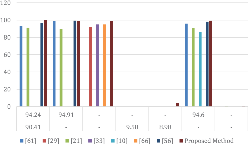
Figure 9: Detection comaprison between proposed and state of art methods

6  Conclusion

Traffic signs are significant for the precise movement of traffic on roads, and the well-being of automobiles, drivers, and pedestrians. Detecting traffic signs, consequently, is gaining prominence gradually, to care about these issues. Researchers have been working for decades to get good results, but still, there is ample space for more improvement. An innovative traffic sign detection methodology is proposed. The proposed method offers a competent, less complicated, and precise methodology for identifying signs. For this purpose, a specific and novel enhancement approach is used with concatenating color features and Haralick features. Quadratic SVM achieved a high rate of classification using these features. 98.5% accuracy is attained using this methodology. The same set of features is used for recognition but there is more work is required, which will be done in the future.

Funding Statement: This work was supported in part by the Basic Science Research Program through the National Research Foundation of Korea (NRF) funded by the Ministry of Education under Grant NRF-2019R1A2C1006159 and Grant NRF-2021R1A6A1A03039493, and in part by the 2022 Yeungnam University Research Grant.

Conflicts of Interest: The authors declare that they have no conflicts of interest to report regarding the present study.

References

1. G. Pappalardo, C. Salvatore, G. D. Alessandro and S. Alessandro, “Decision tree method to analyze the performance of lane support systems,” Sustainability, vol. 13, no. 2, pp. 846, 2021. [Google Scholar]

2. J. Levinson, J. Askeland, J. Becker, J. Dolson, D. Held et al., “Towards fully autonomous driving: Systems and algorithms,” in IEEE Symp. on Intelligent Vehicle, Baden-Baden, Germany, pp. 163–168, 2011. [Google Scholar]

3. B. He, L. Xianjiang, H. Bo, G. Enhui, G. Weijie et al., “UnityShip: A large-scale synthetic dataset for ship recognition in aerial images,” Remote Sensing, vol. 13, no. 24, pp. 4999, 2021. [Google Scholar]

4. Z. Fatin and B. Stanciulescu, “Real-time traffic sign recognition in three stages,” Robotics and Autonomous Systems, vol. 62, no. 1, pp. 16–24, 2014. [Google Scholar]

5. B. Jesús, E. González, P. Arias and D. Castro, “Novel approach to automatic traffic sign inventory based on mobile mapping system data and deep learning,” Remote Sensing, vol. 12, no. 3, pp. 442, 2020. [Google Scholar]

6. D. L. E. Arturo, J. M. Armingol and M. Mata, “Traffic sign recognition and analysis for intelligent vehicles,” Image and Vision Computing, vol. 21, no. 3, pp. 247–258, 2003. [Google Scholar]

7. T. Chen, N. N. Sze, S. Chen, S. Labi and Q. Zeng, “Analysing the main and interaction effects of commercial vehicle mix and roadway attributes on crash rates using a Bayesian random-parameter Tobit model,” Accident Analysis & Prevention, vol. 154, no. 1, pp. 106089, 2021. [Google Scholar]

8. R. Linebaugh, “Colonial fragility: British embarrassment and the so-called migrated archives,” The Journal of Imperial and Commonwealth History, vol. 1, no. 1, pp. 1–28, 2022. [Google Scholar]

9. B. Vaidya and C. Paunwala, “Hardware efficient modified CNN architecture for traffic sign detection and recognition,” International Journal of Image and Graphics, vol. 22, no. 2, pp. 2250017, 2022. [Google Scholar]

10. B. S. Kaplan, H. Gunduz, O. Ozsen, C. Akinlar and S. Gunal, “On circular traffic sign detection and recognition,” Expert Systems with Applications, vol. 48, pp. 67–75, 2016. [Google Scholar]

11. S. H. Hsu and C. L. Huang, “Road sign detection and recognition using matching pursuit method,” Image and Vision Computing, vol. 19, no. 3, pp. 119–129, 2001. [Google Scholar]

12. W. B. Safat, M. A. Abdullah, M. A. Hannan, A. Hussain, S. A. Samad et al., “Vision-based traffic sign detection and recognition systems: Current trends and challenges,” Sensors, vol. 19, no. 9, pp. 2093, 2019. [Google Scholar]

13. L. Chunsheng, S. Li, F. Chang and Y. Wang, “Machine vision based traffic sign detection methods: Review, analyses and perspectives,” IEEE Access, vol. 7, pp. 86578–86596, 2019. [Google Scholar]

14. M. Andreas, M. M. Trivedi and T. B. Moeslund, “Vision-based traffic sign detection and analysis for intelligent driver assistance systems: Perspectives and survey,” IEEE Transactions on Intelligent Transportation Systems, vol. 13, no. 4, pp. 1484–1497, 2012. [Google Scholar]

15. A. S. Alturki, “Traffic sign detection and recognition using adaptive threshold segmentation with fuzzy neural network classification,” in Proc. IEEE ISNCC, Rome, Italy, pp. 1–7, 2018. [Google Scholar]

16. L. Chunsheng, F. Chang, Z. Chen and D. Liu, “Fast traffic sign recognition via high-contrast region extraction and extended sparse representation,” IEEE Transactions on Intelligent Transportation Systems, vol. 17, no. 1, pp. 79–92, 2015. [Google Scholar]

17. Z. Yujun, X. Xu, Y. Fang and K. Zhao, “Traffic sign recognition using deep convolutional networks and extreme learning machine,” in Proc. ICISBDE, Suzhou, China, pp. 272–280, 2015. [Google Scholar]

18. K. T. Phu and L. L. Oo, “RGB color based Myanmar traffic sign recognition system from real-time video,” International Journal of Information Technology (IJIT), vol. 4, no. 4, pp. 12–16, 2018. [Google Scholar]

19. H. Huang and L. Y. Hou, “Traffic road sign detection and recognition in natural environment using RGB color model,” in Proc. ICIC, Liverpool, UK, pp. 345–352, 2017. [Google Scholar]

20. Y. Xue, J. Guo, X. Hao and H. Chen, “Traffic sign detection via graph-based ranking and segmentation algorithms,” IEEE Transactions on Systems, Man, and Cybernetics: Systems, vol. 45, no. 12, pp. 1509–1521, 2015. [Google Scholar]

21. E. Ayoub, M. E. Ansari and I. E. Jaafari, “Traffic sign detection and recognition based on random forests,” Applied Soft Computing, vol. 46, pp. 805–815, 2016. [Google Scholar]

22. J. F. Khan, M. B. Sharif and R. A. Reza, “Image segmentation and shape analysis for road-sign detection,” IEEE Transactions on Intelligent Transportation Systems, vol. 12, no. 1, pp. 83–96, 2010. [Google Scholar]

23. Y. Gu and B. Si, “A novel lightweight real-time traffic sign detection integration framework based on YOLOv4,” Entropy, vol. 24, no. 4, pp. 487, 2022. [Google Scholar] [PubMed]

24. S. Chakraborty and K. Do, “Bangladeshi road sign detection based on YCbCr color model and DtBs vector,” in Proc. ICCIE, Piscataway, New Jersey, US, pp. 158–161, 2015. [Google Scholar]

25. H. Huang and L. Y. Hou, “Speed limit sign detection based on Gaussian color model and template matching,” in Proc. ICVISP, Osaka, Japan, pp. 118–122, 2017. [Google Scholar]

26. C. M. J. Flores, M. A. Sanchez, J. Vargas and M. J. Ayala, “Ecuadorian regulatory traffic sign detection by using HOG features and ELM classifier,” IEEE Latin America Transactions, vol. 19, no. 4, pp. 634–642, 2021. [Google Scholar]

27. S. Abizada, “Traffic sign recognition using histogram of oriented gradients and convolutional neural networks,” in Proc. WCIS, Tashkent, Uzbekistan, pp. 452–459, 2020. [Google Scholar]

28. A. Nabil, S. Rabbi, T. Rahman, R. Mia and M. Rahman, “Traffic sign detection and recognition model using support vector machine and histogram of oriented gradient,” International Journal of Information Technology and Computer, vol. 13, pp. 61–73, 2021. [Google Scholar]

29. K. P. Hosseinzadeh, J. Hyun and E. Kim, “Application of soft histogram of oriented gradient on traffic sign detection,” in Proc. 13th URAI, Xian, China, pp. 388–392, 2016. [Google Scholar]

30. Y. Xue, X. Hao, H. Chen and X. Wei, “Robust traffic sign recognition based on color global and local oriented edge magnitude patterns,” IEEE Transactions on Intelligent Transportation Systems, vol. 15, no. 4, pp. 1466–1477, 2014. [Google Scholar]

31. L. Huaping, Y. Liu and F. Sun, “Traffic sign recognition using group sparse coding,” Information Sciences, vol. 266, pp. 75–89, 2014. [Google Scholar]

32. A. M. Zainal, P. Dhar and K. Deb, “Traffic sign recognition using surf: Speeded up robust feature descriptor and artificial neural network classifier,” in Proc. 9th ICECE, Dhaka, Bangladesh, pp. 198–201, 2016. [Google Scholar]

33. A. Zainal, P. Dhar, M. K. Hossenand and K. Deb, “Traffic sign detection and recognition using fuzzy segmentation approach and artificial neural network classifier respectively,” in Proc. ECCE, Cox’s Bazar, Bangladesh, pp. 518–523, 2017. [Google Scholar]

34. W. C. Chang and C. W. Cho, “Online boosting for vehicle detection,” IEEE Transactions on Systems, Man, and Cybernetics, Part B (Cybernetics), vol. 40, no. 3, pp. 892–902, 2009. [Google Scholar]

35. T. Radu, K. Zimmermann and L. V. Gool, “Multi-view traffic sign detection, recognition, and 3D localisation,” Machine Vision and Applications, vol. 25, no. 3, pp. 633–647, 2014. [Google Scholar]

36. J. G. Park and K. J. Kim, “Design of a visual perception model with edge-adaptive Gabor filter and support vector machine for traffic sign detection,” Expert Systems with Applications, vol. 40, no. 9, pp. 3679–3687, 2013. [Google Scholar]

37. F. Shao, X. Wang, F. Meng, T. Rui, D. Wang et al., “Real-time traffic sign detection and recognition method based on simplified Gabor wavelets and CNNs,” Sensors, vol. 18, no. 10, pp. 3192, 2018. [Google Scholar] [PubMed]

38. E. Li and M. Lingrui, “Traffic sign recognition and retrieval using limited dataset in the wild,” in Proc. IMCEC, Chongqing, China, pp. 1588–1594, 2021. [Google Scholar]

39. M. A. A. Sheikh, A. Kole and T. Maity, “Traffic sign detection and classification using colour feature and neural network,” in Proc. ICICPI, Kolkata, India, pp. 307–311, 2016. [Google Scholar]

40. L. Ming, M. Yuan, X. Hu, J. Li and H. Liu, “Traffic sign detection by ROI extraction and histogram features-based recognition,” in Proc. IJCNN, Dallas, TX, USA, pp. 1–8, 2013. [Google Scholar]

41. M. Vashisht and B. Kumar, “Traffic sign recognition using multi-layer color texture and shape feature based on neural network classifier,” Micro-Electronics and Telecommunication Engineering, vol. 21, no. 1, pp. 479–487, 2021. [Google Scholar]

42. G. Anjan, S. Chokkadi, U. Raghavendra and U. R. Achary, “Local texture patterns for traffic sign recognition using higher order spectra,” Pattern Recognition Letters, vol. 94, no. 15, pp. 202–210, 2017. [Google Scholar]

43. H. Zhiyong, Y. Yu, J. Gu and H. Liu, “An efficient method for traffic sign recognition based on extreme learning machine,” IEEE Transactions on Cybernetics, vol. 47, no. 4, pp. 920–933, 2016. [Google Scholar]

44. P. H. Kassani and A. B. J. Teoh, “A new sparse model for traffic sign classification using soft histogram of oriented gradients,” Applied Soft Computing, vol. 52, pp. 231–246, 2017. [Google Scholar]

45. L. Haojie, F. Sun, L. Liu and L. Wang, “A novel traffic sign detection method via color segmentation and robust shape matching,” Neurocomputing, vol. 169, pp. 77–88, 2015. [Google Scholar]

46. D. G. Lowe, “Distinctive image features from scale-invariant keypoints,” International Journal of Computer Vision, vol. 60, no. 2, pp. 91–110, 2004. [Google Scholar]

47. L. W. Long, X. G. Li, Y. Y. Qin, D. Ma, W. Cui et al., “Real-time traffic sign detection algorithm based on dynamic threshold segmentation and SVM,” Journal of Computers, vol. 31, no. 6, pp. 258–273, 2020. [Google Scholar]

48. R. Cahya, I. F. Rahmah, R. A. Asmara and S. Adhisuwignjo, “Indonesian traffic sign detection and recognition using color and texture feature extraction and SVM classifier,” in Proc. ICOIACT, Yogyakarta, Indonesia, pp. 50–55, 2018. [Google Scholar]

49. Z. Malik and I. Siddiqi, “Detection and recognition of traffic signs from road scene images,” in Proc. 12th Int. Conf. on Frontiers of Information Technology, Islamabad, Pakistan, pp. 330–335, 2014. [Google Scholar]

50. S. S. Gornale, A. K. Babaleshwar and P. L. Yannawar, “Automatic traffic sign detection and classification of Indian traffic signage’s based on multi-feature fusion,” Advances in Cybernetics, Cognition, and Machine Learning for Communication Technologies, vol. 643, no. 1, pp. 209–219, 2020. [Google Scholar]

51. O. S. Kwon, “Speed sign recognition using sequential cascade AdaBoost classifier with color features,” Journal of Multimedia Information System, vol. 6, no. 4, pp. 185–190, 2019. [Google Scholar]

52. W. Wenhao, H. Gao, X. Chen, Z. Yu and M. Jiang, “Traffic sign detection based on Haar and AdaBoost classifier,” Journal of Physics: Conference Series, vol. 1848, no. 1, pp. 012091, 2021. [Google Scholar]

53. K. Bayoudh, R. Knani, F. Hamdaoui and A. Mtibaa, “Transfer learning based hybrid 2D-3D CNN for traffic sign recognition and semantic road detection applied in advanced driver assistance systems,” Applied Intelligence, vol. 51, no. 1, pp. 124–142, 2021. [Google Scholar]

54. X. Liu and F. Xiong, “A real-time traffic sign detection model based on improved Yolov3,” in Proc. IOP-MSE, Ulaanbaatar, Mongolia, vol. 2020, pp. 012034, 2020. [Google Scholar]

55. S. Yin, O. Peng, L. Libo, G. Yike and W. Shaojun, “Fast traffic sign recognition with a rotation invariant binary pattern based feature,” Sensors, vol. 15, no. 1, pp. 2161–2180, 2015. [Google Scholar] [PubMed]

56. L. Shen, Y. Liang, B. Peng and Z. Chuhe, “Group multi-scale attention pyramid network for traffic sign detection,” Neurocomputing, vol. 452, pp. 1–14, 2021. [Google Scholar]

57. C. Xiaochun, C. Zhang, Y. Qian, M. Aloqaily and Y. Xiao, “Deep learning for 5G IoT systems,” International Journal of Machine Learning and Cybernetics, vol. 12, no. 11, pp. 3049–3051, 2021. [Google Scholar]

58. M. Sadiq, S. Daming, G. Meiqin and C. Xiaochun, “Facial landmark detection via attention-adaptive deep network,” IEEE Access, vol. 7, pp. 181041–181050, 2019. [Google Scholar]

59. R. Zhang, I. Akihiro, W. Wenli, S. Benjamin and T. K. Ozan, “Using reinforcement learning with partial vehicle detection for intelligent traffic signal control,” IEEE Transactions on Intelligent Transportation Systems, vol. 22, no. 1, pp. 404–415, 2020. [Google Scholar]

60. A. Gudigar, C. Shreesha, U. Raghavendra and U. R. Acharya, “An efficient traffic sign recognition based on graph embedding features,” Neural Computing and Applications, vol. 31, no. 2, pp. 395–407, 2019. [Google Scholar]

61. Y. Zhu, Z. Chengquan, Z. Duoyou, W. Xinggang, B. Xiang et al., “Traffic sign detection and recognition using fully convolutional network guided proposals,” Neurocomputing, vol. 214, pp. 758–766, 2016. [Google Scholar]

62. R. P. Kumar, M. Sangeeth, K. S. Vaidhyanathan and M. A. Pandian, “Traffic sign and drowsiness detection using open-cv,” IRJET Journal, vol. 6, no. 3, pp. 1398–1401, 2019. [Google Scholar]

63. J. Wan, D. Wei, Z. Hanlin, X. Ming, H. Zunkai et al., “An efficient small traffic sign detection method based on yolov3,” Journal of Signal Processing Systems, vol. 93, no. 8, pp. 899–911, 2021. [Google Scholar]

64. Z. Liu, S. Chao, Q. Mingyuan and F. Xing, “Sadanet: Integrating scale-aware and domain adaptive for traffic sign detection,” IEEE Access, vol. 8, pp. 77920–77933, 2020. [Google Scholar]

65. R. Ayachi, A. Mouna, S. Yahia and A. Mohamed, “Traffic signs detection for real-world application of an advanced driving assisting system using deep learning,” Neural Processing Letters, vol. 51, no. 1, pp. 837–851, 2020. [Google Scholar]

66. Y. Liu, P. Jiyao, J. Xue, Y. Chen and Z. Fu, “TSingNet: Scale-aware and context-rich feature learning for traffic sign detection and recognition in the wild,” Neurocomputing, vol. 447, pp. 10–22, 2021. [Google Scholar]

67. I. W. Selesnick, B. G. Richard and K. C. Nick, “The dual-tree complex wavelet transform,” IEEE Signal Processing Magazine, vol. 22, no. 6, pp. 123–151, 2005. [Google Scholar]

68. J. Darbon, C. Alexandre, C. F. Tony, O. Stanley and J. J. Grant, “Fast non-local filtering applied to electron cryomicroscopy,” in Proc. 5th ISBINM, Paris, France, pp. 1331–1334, 2008. [Google Scholar]

69. S. Houben, S. Johannes, S. Jan, S. Marc and I. Christian, “Detection of traffic signs in real-world images: The German traffic sign detection benchmark,” in Proc. 2013 IJCNN, Dallas, TX, USA, pp. 1–8, 2013. [Google Scholar]