Leveraging Gradient-Based Optimizer and Deep Learning for Automated Soil Classification Model

1  Introduction

Soil classification is the most emanating topic and a major affair in several countries, and its features play a crucial role in estimating different agriculture-relevant jobs and, thus, have an influence on the engineering sector of farming [1]. Perceiving soil features might lay out valuable data to develop well-circumspect management and better logical system and utilize them in farming sectors. Climate, Biota, and ecological antiquity were the major aspect that affected the physical and chemical characteristics of the soil excessively (regional and continental scale), whereas crucial factors would be topography and human activity controls soil characteristics at a minimal level [2]. The important component of soil is the distinct fragments (quartz grains, plant fragments, and clay minerals) that could be observed in disintegration using an optical microscope. Soil structure can be intrinsically linked to the shape, sharpness, voids, spatial arrangement, contrast frequency, and size of crucial particles [3]. Furthermore, a lot of traits are based on the magnification and constituent alignment used. Traditionally, there exist different techniques for determining the colour and texture of the soil. Several approaches for field and laboratory use are the Munsell colour chart method, pipette technique, elutriation technique, and decantation technique [4]. Also, for soil categorization, the triangle technique exists. The disadvantage of this method is such; these are time-consuming and labour-intensive. Thus, soil classification has received considerable interest in the utilization of image processing and computer vision-oriented techniques for soil categorization [5].

Deep learning (DL) is modelled by simulating the anatomical structure of the human brain and has made breakthroughs in applications, including speech recognition and image recognition [6]. The widely applied classification technique, Support Vector Machines (SVMs), is a Machine Learnings (MLs) procedure related to statistical learning concepts. The concept behindhand SVM is that the input sample was projected from lower to higher dimension space through non-linear mapping that allows information in the lower dimensional space that isn’t linearly separable to convert into a linearly separable dataset in the higher dimensional space [7]. In contrast, the DL algorithm is to convert the original signals layer-wise and converts the feature representations in the original to novel feature space. Also, it learns to obtain the hierarchical feature representations automatically, and the classification outcome is accomplished [8]. Convolution Neural Network (CNN) is a network architecture in the DL method that has better effects in the classification of images and makes the CNN technique extensively applied in several domains [9]. CNN is a non-destructive and emerging technique for the applications of quality monitoring of agriculture products, involves the grading and detection of vegetables, fruits, and so on, and has accomplished better outcomes [10]. Usually, CNN is utilized for classification modelling with a larger sample size.

This study introduces a Gradient-Based Optimizer and Deep Learning for Automated Soil Classification (GBODL-ASC) technique. The presented GBODL-ASC technique identifies various kinds of soil using DL and computer vision approaches. In the presented GBODL-ASC technique, three significant processes are involved. At the initial stage, the presented GBODL-ASC technique applies the GBO algorithm with the EfficientNet prototype to generate aspect vectors. For soil categorization, the GBODL-ASC method uses Arithmetic Optimization Algorithms (AOAs) with Back Propagation Neural Networks (BPNNs) model. The design of GBO and AOA algorithms assist in the proper selection of parameter values for the EfficientNet and BPNN models, respectively. To demonstrate the significant soil classification outcomes of the GBODL-ASC methodology, a wide-ranging simulation analysis is performed.

The balance research is arranged in the following. Section 2 defines the literature reviewing, and Section 3 offers the suggested models. Next, Section 4 provides experimental validation, and Section 5 completes the study.

2  Related Works

In [11], an innovative optimized multi-output Generalized Feed-Forward Neural Networks (GFNNs) structure utilizing fifty-eight Piezocone Penetration Test Points (CPTs) to produce a digitalized soil categories map in the South-West region of Sweden was formulated. The presented GFNN structure was assisted by the Generalized Shunting Neurons (GSNs) method calculating units for raising the ability of non-linear restrictions of categorized paradigms. In [12], the author modelled a technique that forecasts soil sequence with land category, and as per the assessment, this can recommend suitable crops. Numerous ML techniques like Gaussian Kernel-based SVM, Weighted K-Nearest Neighbor (k-NN), and Bagged Trees were employed for categorizing soil. In [13], the soil test report values will be employed for classifying numerous soil features like village-wise soil fertility indices of Available Boron (B), Phosphorus (P), Organic Carbon (OC), and Available Potassium (K), along with the parameter Soil Reaction (pH). These five classifier issues were solved with the use of fast learning classifier approach called Extreme Learning Machine (ELM) with various activation functions, namely triangular basis, Gaussian radial basis, hyperbolic tangent, hard limit, and sine-squared.

Escorcia-Gutierrez et al. [14] intend to devise an intellectual soil nutrition and pH categorization utilizing the Weighted Voting Ensemble DL (ISNpHC-WVE) method. The target of devised ISNpHC-WVE approach is to categorize the presence of nutrients and pH levels existing in the soil. Furthermore, 3 DL techniques named Bidirectional Long Short-Term Memory’s (BiLSTMs), Gated Recurrent Units (GRUs), and Deep Belief Networks (DBNs) are employed for predictive analysis. Moreover, the hyper-parameter optimization of 3 DL techniques has been carried out through the manta ray foraging optimization (MRFO) method. Dinh et al. [15] formulated an ML method related to SVM for soil erosion contemplation. The SVM acts as the chief predictive equipment accomplishing a non-linear function that maps take influencing elements for precise forecasts. Additionally, history-related adaptive discrepancy evolution, including Linear Population Size Reduction and Population-Wide Inertia Term (L-SHADE-PWI), was leveraged for identifying the finest set of constraints for SVM for enhancing the prototype’s accuracy.

Vu et al. [16] devise an advanced data-driven approach that depends on the Social Spider Algorithms (SSAs), Metaheuristic and Multivariate Adaptive Regression Splines (MARS), which are used to estimate soil erosion susceptibility. Temporarily, the SSA meta-heuristic was intended to enhance the MARS efficiency by spontaneously tuning its hyperparameter. In [17], a new technique was formulated in this work for zonation and soil classification in 2D vertical cross-section utilizing Cone Penetration Test (CPT). The modelled technique has three main components: soil layer or zone delineation utilizing an edge recognition algorithm, 2D interpolation of CPT Datasets utilizing 2D Bayesian compressive sampling, determining Soil Behavior Type (SBT) utilizing an SBT chart at all locations in the 2D section, which includes areas with unsampled locations and measurements.

3  The Proposed Model

In this research, an automatic soil categorization technique, named GBODL-ASC technique, using DL and computer vision approaches, is presented. In the presented GBODL-ASC technique, three major processes are involved, namely EfficientNet feature extraction, BPNN classification, and parameter optimization. Fig. 1 illustrates the working technique of the GBODL-ASC method.

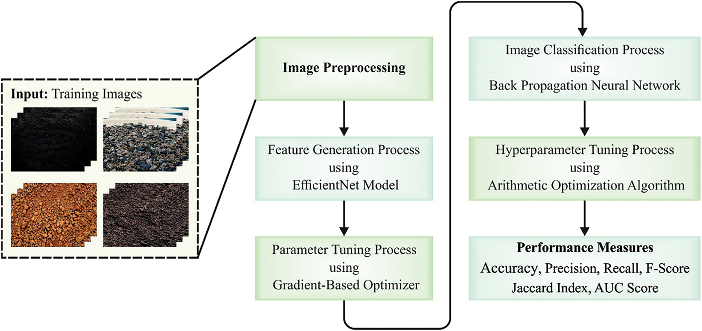
Figure 1: Working procedure of GBODL-ASC method

3.1 Module I: Feature Extraction Process

The introduced GBODL-ASC method applies the EfficientNet model to generate feature vectors. EffcientNet is developed to optimize the efficiency and accuracy of CNN through a uniform scaling mechanism to each dimension, viz., network resolution, depth, and width, yet scaling down the model [18]. Generally, convNet scales up or down by altering the resolution, depth, or width of the network, but scaling individual dimensions of the network augments accuracy. Hence, to accomplish the best efficiency and accuracy, it is significant to uniformly scale each dimension of network depth, width, and resolution.

The compound scale model uses grid searching to discover the associations amongst the distinct scale dimension of the baseline networking in static resource constraints. In the presented technique, an adequate scaling feature for depth, width, and resolution dimension is defined. This coefficient was employed for scaling the baseline networking to the anticipated goal. This kind of structure is named the EfficientNet model, and it has eight dissimilar variations between EfficientNet B0 to EfficientNet B7. The precision of EfficientNet rises explicitly as the procedure count rises. They were termed EfficientNet since they accomplished the best efficiency and accuracy than the preceding CNN.

The essential component of the EfficientNet families can be the inverted bottleneck MBConv that is resulting from MobileNetV2 developed. The block of MBconv was an inverted residual blocking encompassing levels that initially widened and expanded the channel. Hence the straight connection is utilized between bottlenecks that interconnect a less amount of channels when compared to the expansion layer. Additionally, this framework employs in-depth separable convolution that brings down computation by nearly a k2 factor than typical layers, whereas k represents kernel size. For working with inverted residual connection and to enhance accuracy, a novel activation function named Swish activation was utilized rather than the ReLu activation function. To construct the variant of baseline models, distinct values will be replaced for the compound coefficient psi [18].

Depth:d=αψ(1)

Width:w=βψ(2)

resolution:r=γψ(3)

α≥1,β≥1,γ≥1

whereas α, β, γ denotes constant fixed through grid search. ψ represents user-determined coefficients which control how much resources are available for model scaling, whereas α, β, γ define how to assign this extra resource to the resolution, width, and depth of the network correspondingly. With baseline EfficientNet-BO, a compound scaling model can be used to scale up through the subsequent two steps

•   Utilizing determined α, β, γ values as constant enhance baseline networks for creating EfficientNet B1 to B7 with ψ value.

•   Define the better value for α, β, γ by fixing ψ=1 through grid searching with the hypothesis that there exist twice as various resources offered.

Then, the classifier outcomes attained by distinct TL methods are examined. From the outcomes, it is evident that EfficientNet generates best outcomes than others.

To regulate the hyper-parameters associated with the EfficientNet procedure, the GBO technique was exploited. Generally, the GBO stimulates gradient-related Newton’s technique [19]. The GBO is based on two operators for updating the solutions, namely the Gradient Search Rules (GSRs) and the Local Escaping Operators (LEOs). Initially, it is utilized for improving the exploration and then improving the exploitation capability. The primary process in GBO is to create a population X with N solution, generated randomly using Eq. (4) [19]:

χi=χmin+rand×(xmax−xmin),i=1,2,…,N(4)

In Eq. (4), χmin and xmax denote the boundaries of the search space, and rand∈[0,1] indicates the random integer. Next, the fitness values for all the solutions are calculated, and later the better solution is defined. Thus, the direction movement (DM) and gradient search rule (GSR) is employed for updating the solution (xiIi,i=1,2,…,N) in the direction (xb−xiIt) (whereas xb represents the better solution). This updating procedure can be accomplished by calculating x1iIt,x2iIt and x3iIt as follows [19]:

x1iIi=xiIt−GSR+rand×ρ1×(χb−xiIt)(5)

From the expression, ρ1 is utilized for enhancing the balance between exploitation and exploration, and it can be formulated by Eq. (6):

ρ1=2×rand×α−α(6)

whereas:

α=|β×sin(3π/2+sin(β×3π/2))|

β=βmin+(βmax−βmin)×(1−(It/MaxIt)3)2

Now, βmin=0.2 and βmax=1.2. Iter signifies the existing iterations, and MaxIt shows the overall iteration count:

GSR=randn×ρ2×2×Δx×xiItypi−yqi+e(7)

Δx=rand(1:N)×|((xb−xr1It)+δ)/2|

δ=2×rand×(|(xr1Ii+xr2It+xr3It+xr4It)/4−xiIt|)

where rand(1: N) represent a random vector whose dimensions, r1,r2,r3, and r4, indicate random number within [1, N]. ypi and yqi positions are upgraded as follows [19]:

ypi=rand×(xs+χi)/2+rand×Δx(8)

yqi=rand×xs+xiIt2−rand×Δx(9)

xs=xiIt−randn×ρ1×2×Δx×xiItxb−xworst+e(10)

x2iIt=χb−GSR+rand×ρ2×(xr1It−xr2It)(11)

x3iIi=xiIt−ρ1×(x1iIt−x2iIi)(12)

By using x1iIt,x2iIt, and x3iIt positions, a new solution at It+1 iteration can be attained:

xiIt+1=ra×(rb×x1iIi+(1−rb)×x2iIi)+(1−ra)×x3iIi(13)

In Eq. (13), ra and rb represent two random values. Furthermore, the LEO is employed for improving the exploitation capability of GBO. This can be accomplished by upgrading the solution xiIt through the subsequent formula based on pr probability:

xiIt+1={xiIt+f1×W1+f2×ρ1×W3+u2×W2/2pr<0.5χb+f1×W1+f2×ρ1×W3+u2×W2/2otherwise(14)

W1=(u1×xb−u2×xkIt),

W2=(xr1Ii−xr2It),

W3=(u3×(x2iIt−x1iIt))

Now, f1∈[−1,1] and f2 correspondingly denotes a random integer and u1, u2, and u3 indicates three random values determined by the following expression:

u1=L1×2×rand+(1−L1)(15)

u2=L1×rand+(1−L1)

u3=L1×rand+(1−L1)

whereas L1 indicates a binary variable (assigned to zero or one). Thus, the novel solution can be attained through the succeeding formula:

xkIt=L2×xpIt+(1−L2)×xrand(16)

In Eq. (16), L2 is the same as L−1, xpIt indicates the solution selected from X, and xrand represents a random solution attained by Eq. (4).

3.2 Module II: Soil Classification Process

For soil classification, the feature vectors are passed into the BPNN prototype. The BPNN is a NN form that is extensively applied in different scenarios due to its self-adaptive capabilities and stronger non-linear mapping [20]. It comprises implicit, output, and input layers. Where O signifies the output and xj represents the input. Fig. 2 depicts the infrastructure of BPNN. Meanwhile, the output is a score, the number of outputs is fixed as 1, and the input comprises of distinct index dataset, and the number of inputs is fixed as 13, and it can be framed as mentioned in the following [20]:

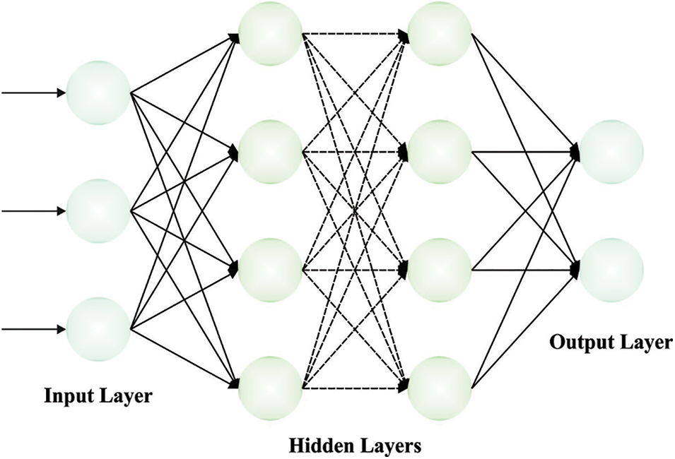
Figure 2: Structure of BPNN

hid−num=m+n+a(17)

In Eq. (17), hid−num indicates the neuron count in the Hidden Layer (HL), m denotes the neuron number in the input layer, n indicates the neuron count in the output layer, and a indicates an integer with 1≤a≤10. Afterwards, defining the fundamental architecture of the NN, the nodes of the input and output in the HL are consequently computed. The input of j-th neurons in the HL is evaluated as follows [20]:

Hidj=∑i=1nwijxj−θi1(18)

In Eq. (18), n indicates the input count, wij denotes the connecting line weight from i-th to j-th neurons, xj shows the input value, and θi1 indicates the threshold value of j-th HL, and it can be expressed as follows [20]:

Oj=f(∑j=1nwijxj−θ61j)(19)

In Eq. (19), function f represents the excitation function, and it is given in the following expression:

y=∑i=1kwjOj+θ2(20)

Finally, the BPNN parameters can be chosen optimally by the AOA. AOA uses mathematical operators in arithmetic [21]. AOA provides an uncomplicated application that is regulated to overcome novel optimization problems. Also, AOA does not require altering several parameters. Similarly, the AOA’s parameters of random and adaptive hastened the convergence and divergence of searching resolutions. The fundamental AOA operations are exploitation, initialization, and exploration.

(a) Initialization. As demonstrated in Eq. (21), candidate solutions (XA) are arbitrarily produced. The existing populace can be denoted as the matrix XA. The dimension is represented as DM. The number of persons can be indicated as NP as follows [21].

XA=[xa1,1⋯xa1,DM−1xa1,DMxa2,1⋯xa2,DM−1xa2,DM⋮⋯⋮⋮xaNP,1⋯xaNP,DM−1xaNP,DM](21)

The search phrase was selected as an exploitation or exploration stage with the use of the math optimizer accelerated (MOA) function in Eq. (22).

MOA(iter)=miniter+iter×(maxiter−miniterMiter),(22)

whereas Miter indicates the maximal amount of iterations. The existing iteration can be represented as iter. The minimal and maximal MOA values represent miniter and maxiter correspondingly. miniter and maxiter are variables and fixed as 0.2 and 1, correspondingly.

(b) Exploration. When r1>MOA(r1 represents an arbitrary value), the Division (D) or Multiplication (M) operators are performed [21].

xai,j(iter+1)={best(xaj)÷(MOP+ε)×((UBj−LBj)×μ+LBj),r2>0.5best(xaj)×MOP×((UBj−LBj)×μ+LBj),r2≤0.5′(23)

whereas r2 indicates a random integer. Best(xa) indicates the j-th location in the optimum solution. ε represents a smaller value. The upper and lower limits of the j-th location are indicated as UBj, and LBj.μ are fixed as 0.5.

MOP(iter)=1−iter1/αMiter1/α′(24)

whereas α denotes the sensitive parameter that is set equivalent to 5.

(c) Exploitation. When r1≤MOA, the Subtraction (S) or Addition (A) operators are performed [21].

xai,j(iter+1)={best(xaj)−MOP×((UBj−LBj)×μ+LBj),r3>0.5best(xaj)+MOP×((UBj−LBj)×μ+LBj),r3≤0.5(25)

Lastly, the optimum solution for the existing iteration is the best. The current optimal fitness is related to the preceding better fitness, and the lowest values are applied to compute the final optimum solution.

The AOA algorithm makes Fitness Function (FF) derivation to get an enhanced categorizer result. It defines positive values as indicating the superior result of the candidate’s resolutions. In this study, the mitigated categorizer error rate will be regarded as the FF, as demonstrated in Eq. (26) [21].

fitness(xi)=ClassifierErrorRate(xi)=number of misclassified samplestotal number of samples∗100(26)

4  Experimental Validation

In this segment, the experimental validation of the GBODL-ASC method on the soil classification process is well studied on a dataset [22] comprising 156 images and five classes, as defined in Table 1. Fig. 3 illustrates the trial pictures. The dataset includes images with 300 dpi resolution, 250 m spatial resolution, three band spectral resolution, RGB colour system, and three channels.

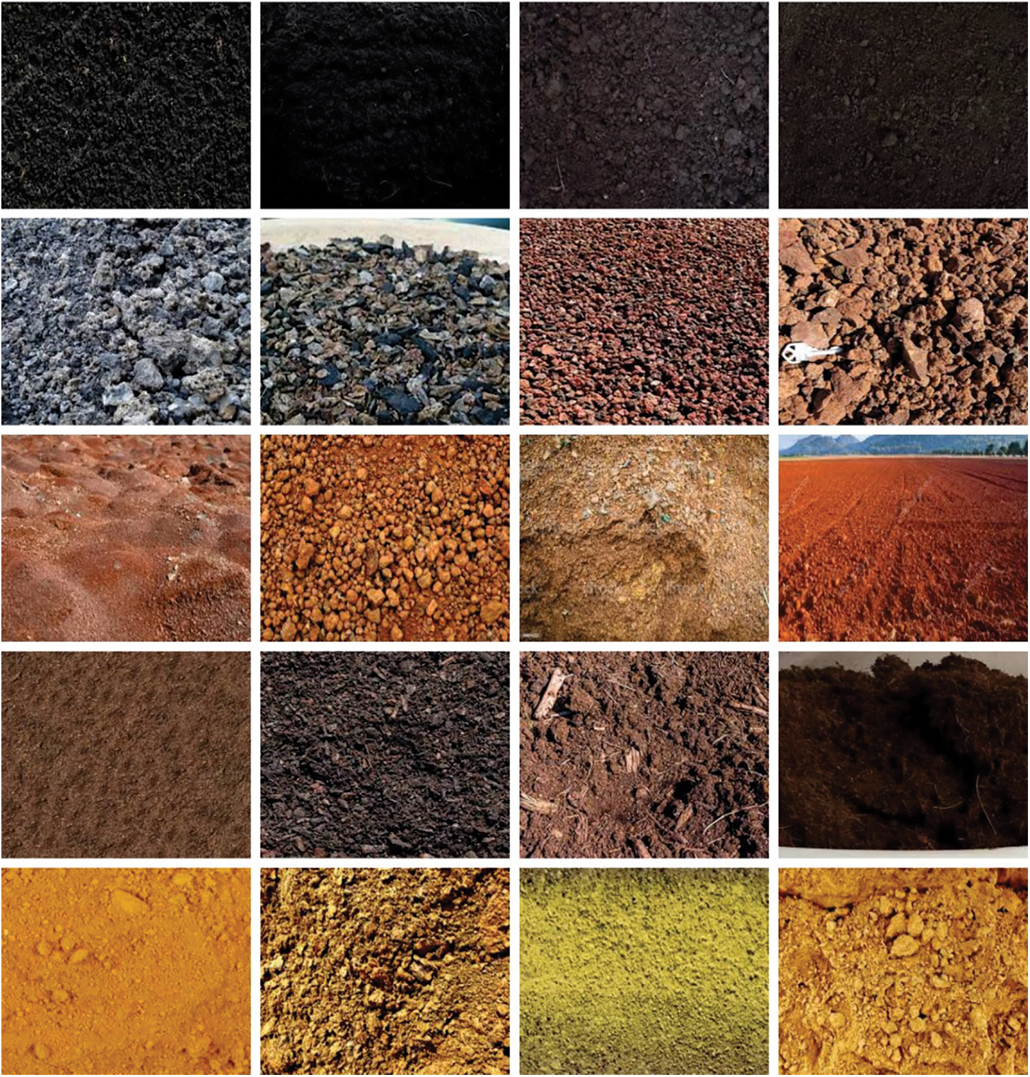
Figure 3: Sample images

The soil categorization results of the GBODL-ASC model under distinct epochs are represented in Fig. 4. The figure accentuated that the GBODL-ASC procedure has recognized five different kinds of soil. On epoch 50, the GBODL-ASC model has categorized 25 samples into Black, 18 samples into Cinder, 21 samples into Laterite, 12 samples into Peat, and 13 samples into Yellow. Moreover, on epoch 200, the GBODL-ASC approach has categorized 31 samples into Black, 23 samples into Cinder, 23 samples into Laterite, 26 samples into Peat, and 25 samples into Yellow. Furthermore, on epoch 250, the GBODL-ASC system has categorized 30 samples into Black, 24 samples into Cinder, 26 samples into Laterite, 26 samples into Peat, and 24 samples into Yellow. At last, on epoch 300, the GBODL-ASC technique has categorized 31 samples into Black, 25 samples into Cinder, 28 samples into Laterite, 27 samples into Peat, and 28 samples into Yellow.

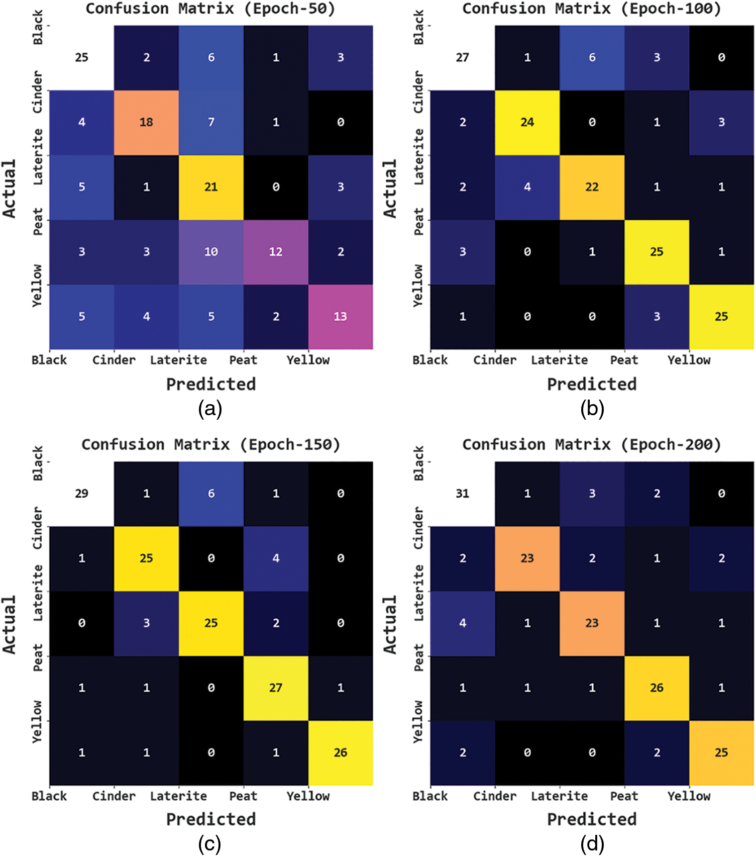
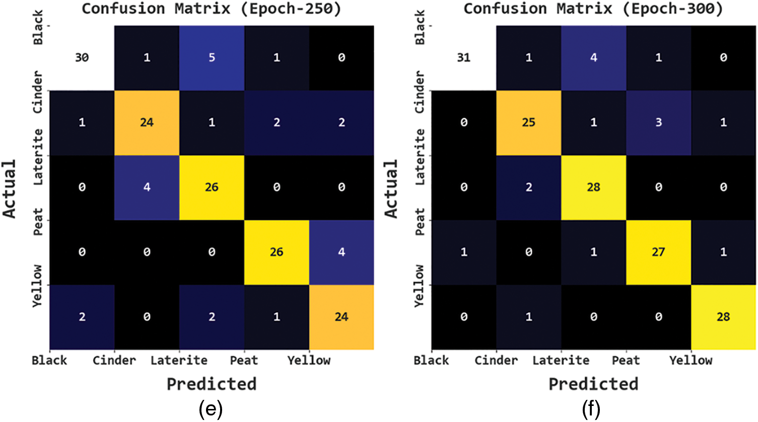
Figure 4: Confusion matrices of GBODL-ASC structure (a) Epoch50, (b) Epoch100, (c) Epoch150, (d) Epoch200, (e) Epoch250, and (f) Epoch300

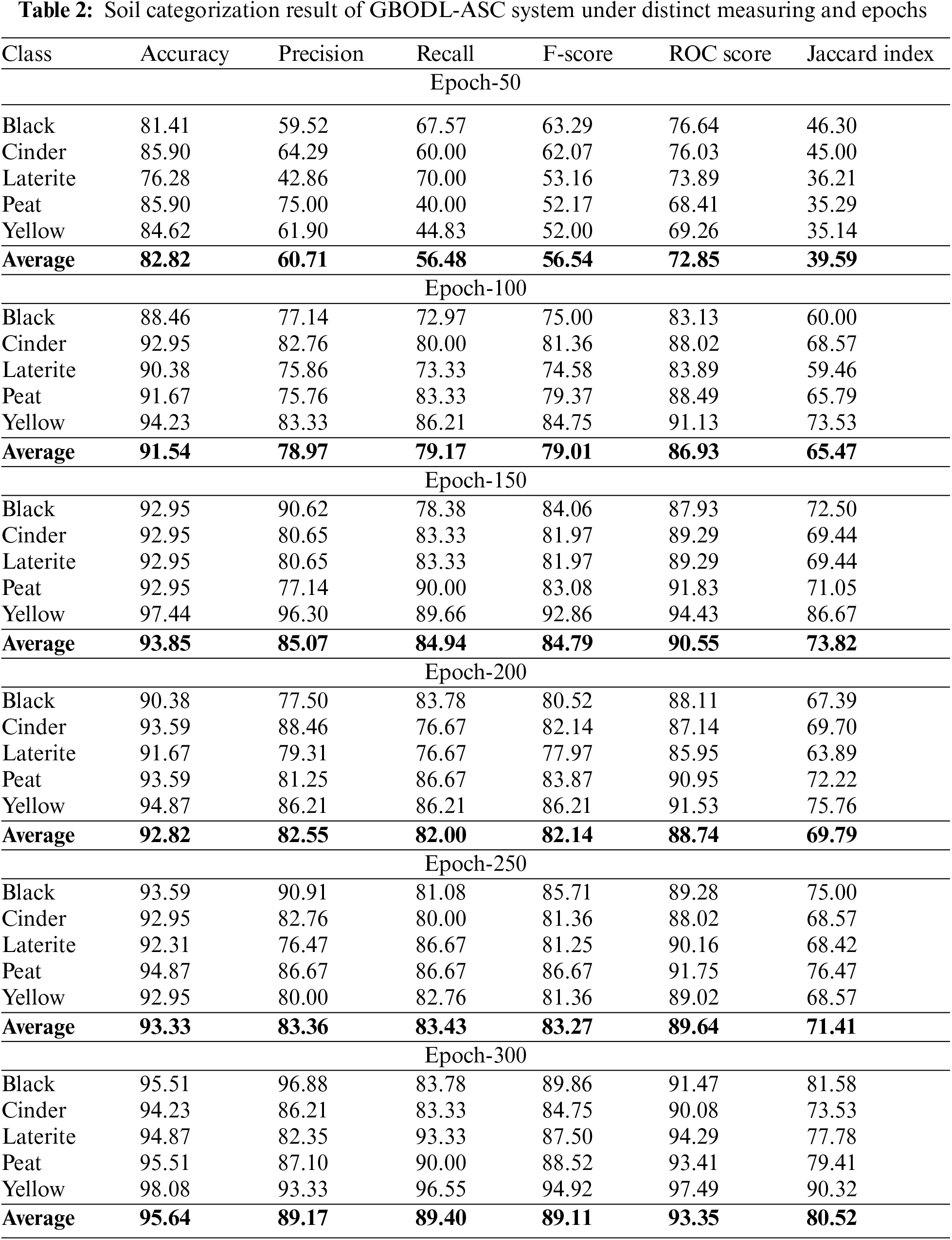
Table 2 reports a brief set of soil classification outcomes of the GBODL-ASC model under distinct epochs. The experimental values signified the GBODL-ASC model had obtained improved outcomes under every epoch. For instance, on 50 epochs, the GBODL-ASC model has attained an average accuy of 82.82%, precn of 60.71%, recal of 56.48%, Fscore of 56.54%, receiver operating characteristic (ROC) curve ROCscore of 72.85%, and Jaccardindex of 39.59%. Also, on 100 epochs, the GBODL-ASC system has reached an average accuy of 91.54%, precn of 78.97%, recal of 79.17%, Fscore of 79.01%, ROCscore of 86.93%, and Jaccardindex of 65.47%. Along with that, on 200 epochs, the GBODL-ASC technique has accomplished an average accuy of 92.82%, precn of 82.55%, recal of 82%, Fscore of 82.14%, ROCscore of 88.74%, and Jaccardindex of 69.79%. Finally, on 300 epochs, the GBODL-ASC system has achieved an average accuy of 95.64%, precn of 89.17%, recal of 89.40%, Fscore of 89.11%, ROCscore of 93.35%, and Jaccardindex of 80.52%.

The Training Accuracy (TACC) and Validation Accuracy (VACC) of the GBODL-ASC procedure under distinct epochs are evaluated on soil categorization achievement in Fig. 5. The image pointed out that the GBODL-ASC algorithm has demonstrated precipitated accomplishment with precipitated values of TACC and VACC. It is noticeable that the GBODL-ASC system has attained higher TACC results.

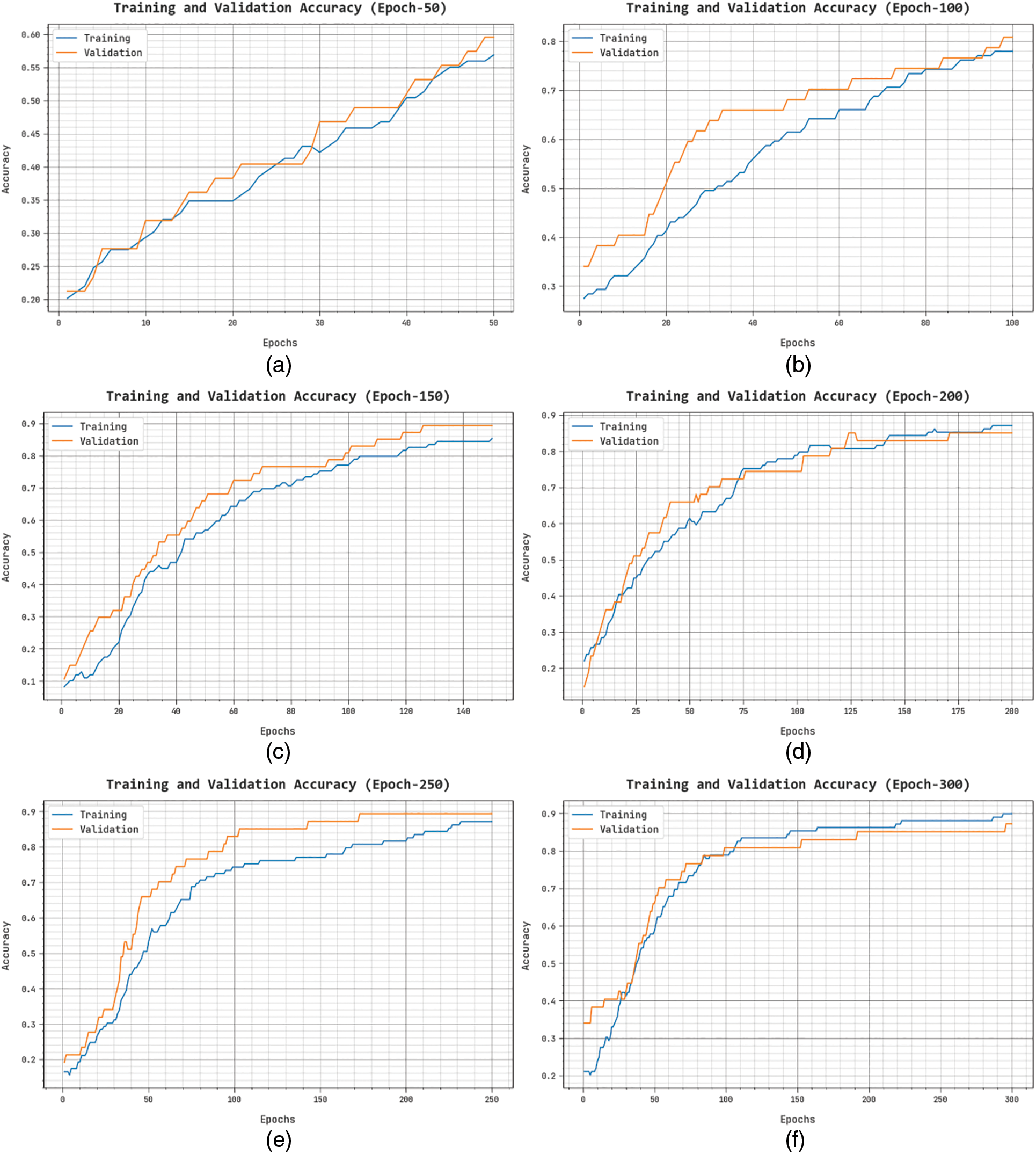
Figure 5: TACC and VACC analysis of GBODL-ASC system

The Training Loss (TLS) and Validation Loss (VLS) of the GBODL-ASC system under varying epochs on soil classification accomplishment in Fig. 6. The image referred that the GBODL-ASC procedure has exhibited optimum accomplishment with lessened TLS and VLS values. The GBODL-ASC methodology has given an outcome in reduced VLS results.

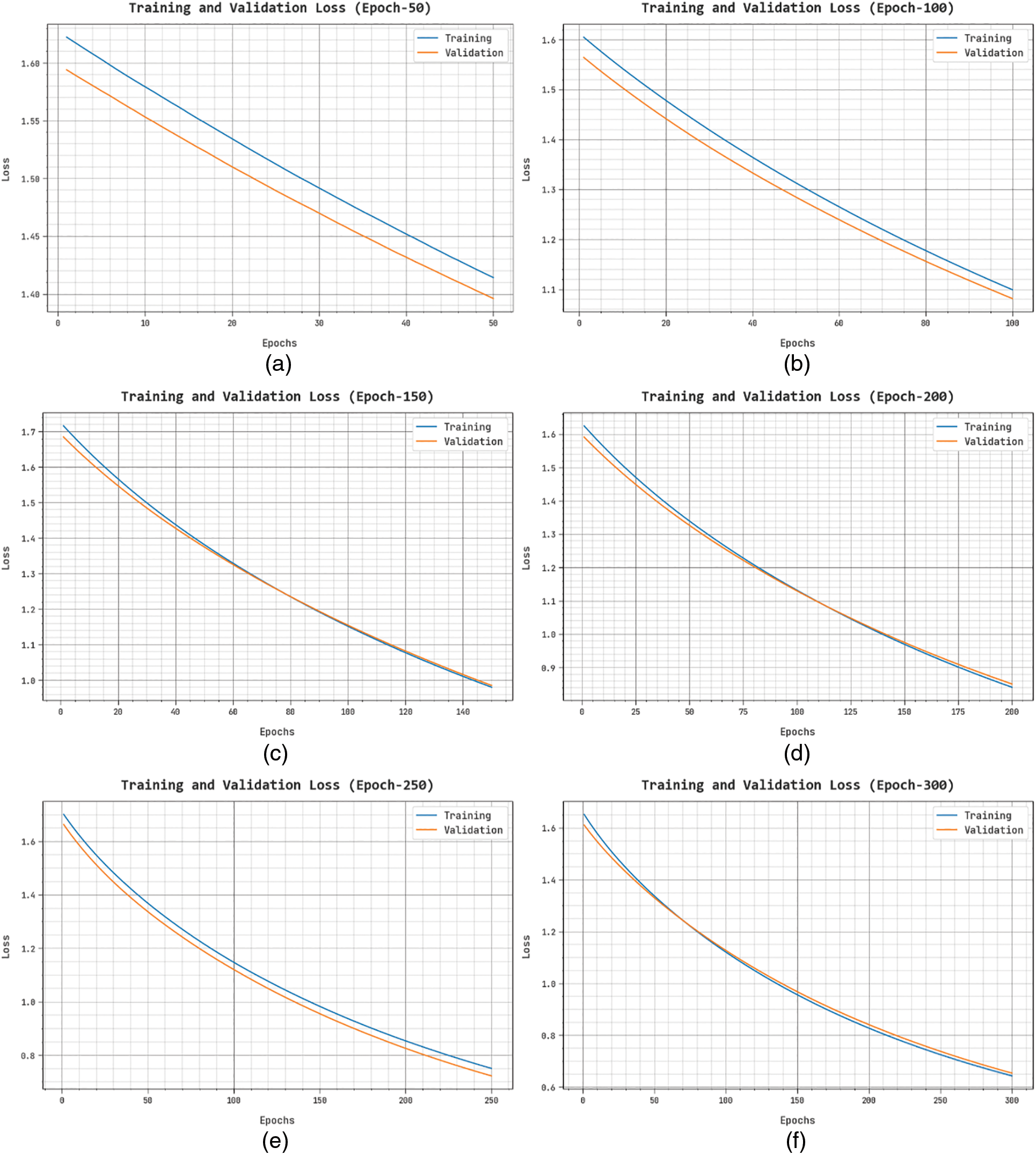
Figure 6: Evaluation of TLS and VLS GBODL-ASC technique

An apparent precision-recall analysis of the GBODL-ASC system in distinct epochs is described in Fig. 7. specified that the GBODL-ASC procedure had given an outcome in greater precision-recall values in several categories.

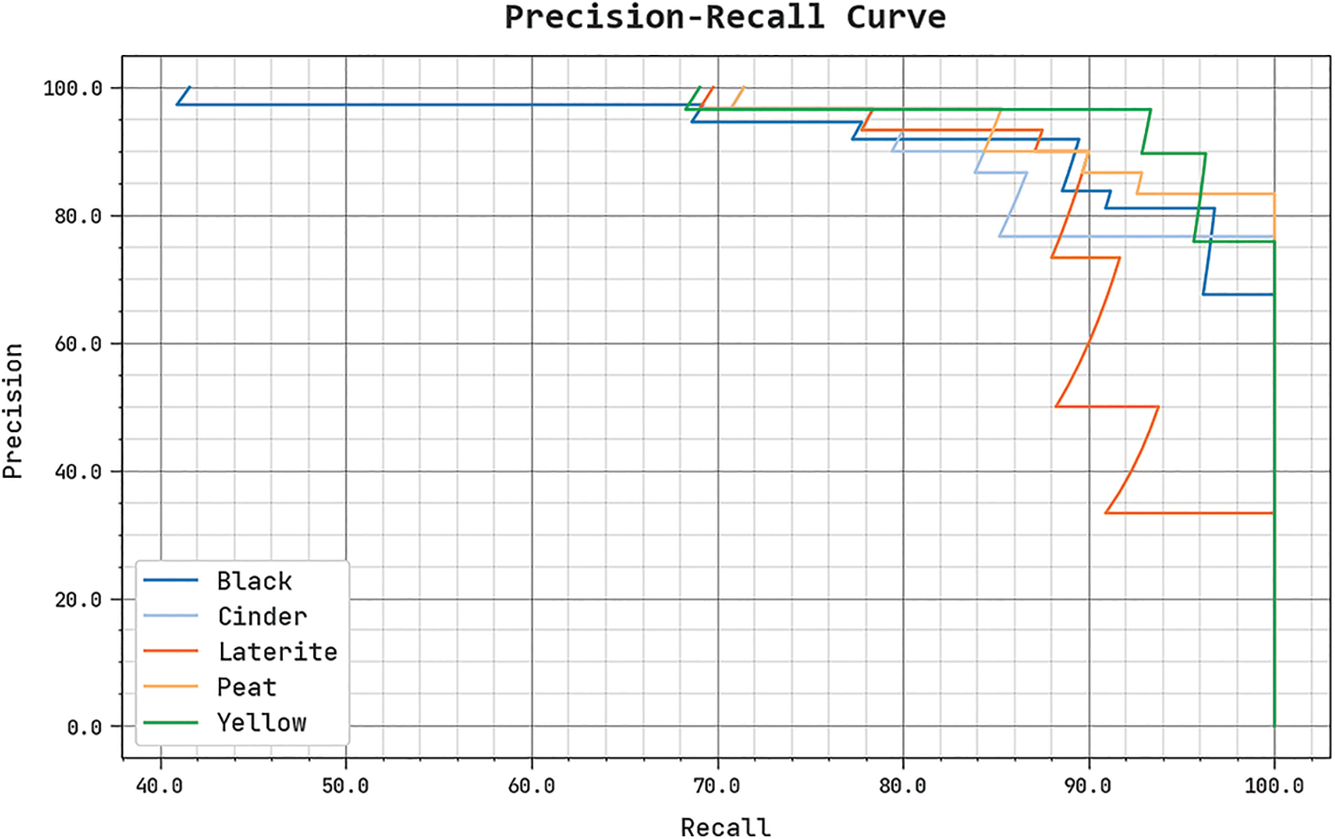
Figure 7: Precision-recall investigation of the GBODL-ASC method

An overall ROC research of the GBODL-ASC approach in distinct epochs is illustrated in Fig. 8. The result emphasized by the GBODL-ASC method has exposed its capability in cataloguing in several classes.

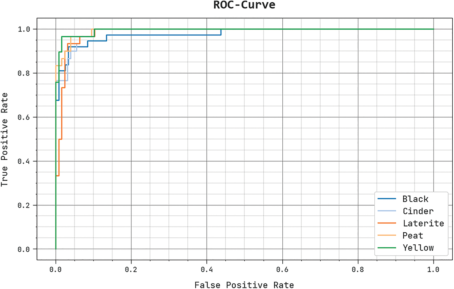
Figure 8: ROC curve inspection of GBODL-ASC method

Comparative soil classification results of the GBODL-ASC method with recent methods are portrayed in Table 3. The obtained values inferred the betterment of the GBODL-ASC model compared to recent methods. For example, based on accuy, the GBODL-ASC method has obtained an improved accuy of 95.64% while the Particle Swarm Optimization (PSO), Gravitational Search Algorithm (GSA), Decision Tree (DT3), Artificial Neural Network (ANN), SVM, and hybrid Fuzzy C-Means with Crow Search Optimization (FCM-CSO) models have reached reduced accuy of 76.30%, 77.20%, 87.99%, 88.81%, 88.64%, and 94.32% respectively.

Also, concerning precn, the GBODL-ASC approach has reached an enhanced precn of 89.17% while the PSO, GSA, DT3, ANN, SVM, and hybrid FCM-CSO approaches have attained lower precn of 78.10%, 78.54%, 86.12%, 87.23%,86.72%, and 89.15% appropriately. These outcomes guaranteed the capability of the GBODL-ASC prototype in the automated soil classification process.

5  Conclusion

In this study, an automated soil classification technique is introduced, named the GBODL-ASC technique using DL and computer vision approaches. In the presented GBODL-ASC technique, three major processes are involved. At the initial stage, the presented GBODL-ASC technique applies the GBO algorithm with the EfficientNet procedure to generate feature vectors. For soil categorization, the GBODL-ASC procedure uses an AOA with the BPNN model. The design of GBO and AOA algorithms assist in the proper selection of parameter values for the EfficientNet and BPNN models, respectively. To demonstrate the significant soil classification outcomes of the GBODL-ASC method, a wide-ranging simulation analysis is performed. The experimental outcomes show an enhanced GBODL-ASC model than other techniques.

Funding Statement: Princess Nourah bint Abdulrahman University Researchers Supporting Project number (PNURSP2023R303), Princess Nourah bint Abdulrahman University, Riyadh, Saudi Arabia. Research Supporting Project number (RSPD2023R787), King Saud University, Riyadh, Saudi Arabia. This study is supported via funding from Prince Sattam bin Abdulaziz University project number (PSAU/2023/R/1444).

Conflicts of Interest: The authors declare that they have no conflicts of interest to report regarding the present study.

References

1. S. W. Moon, R. E. Kim, A. C. Cheng, Y. E. Li and T. Ku, “Post-processing of background noise from SCPT auto source signal: A feasibility study for soil type classification,” Measurement, vol. 156, pp. 107610, 2020. [Google Scholar]

2. A. Pandey, D. Kumar and D. B. Chakraborty, “Soil type classification from high resolution satellite images with deep CNN,” in IEEE Int. Geoscience and Remote Sensing Symp. IGARSS, Brussels, Belgium, pp. 4087–4090, 2021. [Google Scholar]

3. P. Han, D. Dong, X. Zhao, L. Jiao and Y. Lang, “A smartphone-based soil color sensor: For soil type classification,” Computers and Electronics in Agriculture, vol. 123, pp. 232–241, 2016. [Google Scholar]

4. B. T. Pham, T. A. Hoang, D. M. Nguyen and D. T. Bui, “Prediction of shear strength of soft soil using machine learning methods,” Catena, vol. 166, pp. 181–191, 2018. [Google Scholar]

5. V. Khullar, S. Ahuja, R. G. Tiwar and A. K. Agarwa, “Investigating efficacy of deep trained soil classification system with augmented data,” in 9th Int. Conf. on Reliability, Infocom Technologies and Optimization (Trends and Future Directions) (ICRITO), Noida, India, pp. 1–5, 2021. [Google Scholar]

6. J. I. Colombo, J. Wilches and R. Leon, “Seismic fragility of legged liquid storage tanks based on soil type classifications,” Journal of Constructional Steel Research, vol. 192, pp. 1–15, 2022. [Google Scholar]

7. S. Inazumi, S. Intui, A. Jotisankasa, S. Chaiprakaikeow and K. Kojima, “Artificial intelligence system for supporting soil classification,” Results in Engineering, vol. 8, pp. 100188, 2020. [Google Scholar]

8. Y. Wang, Y. Hu and T. Zhao, “CPT-based subsurface soil classification and zonation in a 2D vertical cross-section using Bayesian compressive sampling,” Canadian Geotechnical Journal, vol. 57, no. 7, pp. 947–958, 2020. [Google Scholar]

9. A. Dornik, L. DRĂGUŢ and P. Urdea, “Classification of soil types using geographic object-based image analysis and random forests,” Pedosphere, vol. 28, no. 6, pp. 913–925, 2018. [Google Scholar]

10. B. B. Bezabeh and A. D. Mengistu, “The effects of multiple layers feed-forward neural network transfer function in digital based ethiopian soil classification and moisture prediction,” International Journal of Electrical and Computer Engineering, vol. 10, no. 4, pp. 4073, 2020. [Google Scholar]

11. A. Ghaderi, A. A. Shahri and S. Larsson, “An artificial neural network based model to predict spatial soil type distribution using piezocone penetration test data (CPTu),” Bulletin of Engineering Geology and the Environment, vol. 78, no. 6, pp. 4579–4588, 2019. [Google Scholar]

12. S. A. Z. Rahman, K. C. Mitra and S. M. Islam, “Soil classification using machine learning methods and crop suggestion based on soil series,” in 21st Int. Conf. of Computer and Information Technology (ICCIT), Dhaka, Bangladesh, pp. 1–4, 2018. [Google Scholar]

13. M. S. Suchithra and M. L. Pai, “Improving the prediction accuracy of soil nutrient classification by optimizing extreme learning machine parameters,” Information Processing in Agriculture, vol. 7, no. 1, pp. 72–82, 2020. [Google Scholar]

14. J. Escorcia-Gutierrez, M. Gamarra, R. Soto-Diaz, M. Pérez, N. Madera et al., “Intelligent agricultural modelling of soil nutrients and pH classification using ensemble deep learning techniques,” Agriculture, vol. 12, no. 7, pp. 977, 2022. [Google Scholar]

15. T. V. Dinh, H. Nguyen, X. L. Tran and N. D. Hoang, “Predicting rainfall-induced soil erosion based on a hybridization of adaptive differential evolution and support vector machine classification,” Mathematical Problems in Engineering, vol. 2021, pp. 1–20, 2021. [Google Scholar]

16. D. T. Vu, X. L. Tran, M. T. Cao, T. C. Tran and N. D. Hoang, “Machine learning based soil erosion susceptibility prediction using social spider algorithm optimized multivariate adaptive regression spline,” Measurement, vol. 164, pp. 108066, 2020. [Google Scholar]

17. Y. Wang, Y. Hu and T. Zhao, “Cone penetration test (CPT)-based subsurface soil classification and zonation in two-dimensional vertical cross section using Bayesian compressive sampling,” Canadian Geotechnical Journal, vol. 57, no. 7, pp. 947–958, 2020. [Google Scholar]

18. S. M. Jaisakthi, C. Aravindan and R. Appavu, “Classification of skin cancer from dermoscopic images using deep neural network architectures,” Multimedia Tools and Applications, vol. 82, no. 10, pp. 1–16, 2022. https://doi.org/10.1007/s11042-022-13847-3 [Google Scholar] [PubMed] [CrossRef]

19. I. Ahmadianfar, O. B. Haddad and X. Chu, “Gradient-based optimizer: A new metaheuristic optimization algorithm,” Information Sciences, vol. 540, pp. 131–159, 2020. [Google Scholar]

20. J. Yu, D. Li, A. Wang, P. Liu, J. Song et al., “An improved evaluation model for supplier selection based on particle swarm optimisation-back propagation neural network,” IET Collaborative Intelligent Manufacturing, vol. 4, no. 4, pp. 316–325, 2022. https://doi.org/10.1049/cim2.12067 [Google Scholar] [CrossRef]

21. M. Obayya, M. S. Alamgeer, J. Alzahrani, R. N. Alabdan, F. Al-Wesabi et al., “Artificial intelligence driven biomedical image classification for robust rheumatoid arthritis classification,” Biomedicines, vol. 10, no. 11, pp. 2714, 2022. [Google Scholar] [PubMed]

22. https://www.kaggle.com/code/prasanshasatpathy/soil-type-image-classification/data [Google Scholar]