Unsupervised Anomaly Detection Approach Based on Adversarial Memory Autoencoders for Multivariate Time Series

1  Introduction

With the widespread adoption of CPSs [1] and the Internet of Things (IoT) in power systems, water treatment plants, pipeline networks, and large-scale computer equipment, the number of interconnected devices and sensors that generate massive amounts of time series data has rapidly increased. It is critical for operators to accurately identify anomalies in these time series to conduct investigations and resolve potential problems [2]. Initial anomaly detection methods relied heavily on domain expert knowledge and statistical methods such as time series decomposition and transformation models [3,4]. Later, as machine learning developed, scientists proposed statistical machine learning-based anomaly detection methods, such as the Autoregressive Integrated Moving Average model (ARIMA), One-Class Support Vector Machine (OC-SVM), Local Outlier Factor (LOF), and K-means clustering (K-means) [5–8]. However, as the complexity of time series data increases and noise interferes, the preceding methods have proved unable to meet the needs of some real production scenarios. With the sharp rise in research on deep learning, deep learning-based anomaly detection methods for temporal data have become a popular field. Many deep learning-based anomaly detection methods have been produced.

Deep learning-based methods include supervised learning methods and unsupervised learning methods. Scholars have shown that supervised learning methods effectively detect known types of anomalies. However, due to the rarity and variety of anomalies, creating training datasets for supervised methods can take time and effort [9]. In addition, supervised methods cannot detect abnormal patterns not contained in training datasets. Therefore, studies in recent years have focused more on unsupervised methods. Reconstruction-based methods [10] are the most common of the unsupervised methods. During the training phase, an encoder-decoder model is typically trained on a training dataset containing only normal data. During the testing phase, this research obtains the reconstruction error of all samples in the test dataset and distinguishes between normal and abnormal samples based on the threshold. All reconstruction-based methods assume that the model can only reconstruct normal samples and not abnormal samples. The deep network model can reconstruct some abnormal samples due to its strong generalization ability, which means that the model does not obtain a significant difference in reconstruction error between normal samples and these abnormal samples on the test dataset, thereby failing to detect this part of the abnormality.

In order to deal with the above problems, this research proposes an unsupervised anomaly detection approach based on adversarial memory autoencoders for multivariate time series. Specifically, a memory module is introduced between the traditional encoder and decoder to learn typical patterns of normal samples to detect abnormal samples that can be easily reconstructed as normal samples. When updating feature vectors, this research allows forgetting partial information to restrain model overgeneralization, which helps to enlarge the reconstruction error of abnormal samples. The model contains three components: an encoder, a memory module, and two decoders. Firstly, an encoder encodes the original input data as a feature vector. Then, a memory module whose parameters can be automatically updated as the model backpropagates is proposed. This memory module is used to learn the prototype patterns of the feature vector and update the feature vector. Finally, two decoders are used to reconstruct the input data and calculate the reconstruction error. To further amplify the reconstruction error of normal and abnormal samples, this research uses an adversarial training strategy during training and the POT [11] method to automatically determine the threshold value to distinguish normal and abnormal samples. The main contributions of this study are as follows:

•   This research proposes a memory module that parameters can update automatically to learn the feature vector’s prototype patterns. This research uses this memory module to update the feature vector to restrain model overgeneralization, which helps detect abnormal samples close to normal.

•   This research introduces adversarial training in the training process to amplify the reconstruction error difference between normal and abnormal samples, making it easier to distinguish between normal and abnormal samples.

•   This research uses the POT method to automatically determine thresholds and demonstrate the effectiveness of the proposed method on a synthetic dataset and four real-world datasets.

The rest of this paper is organized as follows. Section 2 discusses the related work on multivariate time series anomaly detection. Section 3 presents the details of our proposed method. In Section 4, the experiments and effect analysis of the proposed method are given. Finally, Section 5 concludes the work of this paper.

2  Related Work

Time series anomaly detection is a standing research topic among scholars, and many research methods are proposed yearly. This research classifies mainly statistical machine learning and deep learning-based methods.

Statistical machine learning-based methods include modeling the distribution of time series using regression models [12,13], Support Vector Machine (SVM) [14,15], LOF [16,17], and K-means [18]. The authors of [12] proposed using the ARIMA model for anomaly detection of gas consumption and power plant data. The authors of [14] proposed using the OC-SVM model to learn the bounds of normal samples in the training dataset and use them to detect anomalous samples in the test dataset. The authors of [16] proposed using the LOF model to calculate the score of abnormality of each sample based on its dispersion with nearby samples and use this score to distinguish between normal and abnormal samples. The authors of [18] proposed using the K-means model to cluster the samples and consider the ones that significantly deviate from most samples as abnormal. In addition, some models are based on other methods. The authors of [19] utilized the Principal Composition Analysis (PCA) to reduce the dimensionality of multivariate time series data and identify abnormal samples based on the cumulative contribution rate. The authors of [20] utilized Hidden Markov Models (HMM) to model the time series and used the prediction error to identify anomalous samples. Merlin discriminates anomalies by iteratively comparing subsequences of different lengths with the similarity to their neighboring subsequences [21]. Although these methods are fast and versatile in operating well, with the increasing dimensionality and noise interference of time series data, statistical machine learning-based methods are no longer well suited for real-world production needs.

With the development of deep learning in recent years, various advanced deep learning methods have been applied to the anomaly detection task for time series. The main methods include Recurrent Neural Network (RNN)-based methods [22,23], autoencoder-based methods [24,25], Generative Adversarial Network (GAN)-based methods [2,26], Graph Neural Network (GNN)-based methods [27,28], and transformer-based methods [29,30].

The Long Short-Term Memory network-Nonparametric Dynamic Thresholding (LSTM-NDT) method used a Long Short-Term Memory (LSTM) network to learn the temporal correlation of time series data and iteratively predict the next moment sample of the input sample and proposed a Nonparametric Dynamic Thresholding (NDT) strategy to calculate the threshold. It used the gating mechanism to capture time dependency information for anomaly detection at the current moment. However, the training speed of this method is slow when the data input is long, and this method of automatically determining the threshold value is poorly adapted to different scenarios [22]. The Deep Autoencoding Gaussian Mixture Model (DAGMM) organically combined the dimensionality reduction process and density estimation process by considering the density distribution of the autoencoder and gaussian mixture model for end-to-end joint training to avoid the model falling into local optimum due to the two independent steps. It used the decoder to reconstruct the dimensionally reduced data and perform density estimation, which expands the capacity of the model and improves the accuracy of anomaly detection. However, it cannot explicitly capture the correlation between different features [24]. The Deep Convolutional Autoencoding Memory (CAE-M) network combined Convolutional Neural Network (CNN) and LSTM to capture local and temporal features and discriminated abnormal samples by reconstruction errors. It utilized both temporal and spatial information to obtain more accurate anomaly detection results. However, the computational cost is high due to using both CNN and LSTM [25]. The Unsupervised Anomaly Detection for multivariate time series (USAD) used a simple composition of one encoder and two decoders. It used an adversarial training strategy during the training process to obtain better and more stable training results than autoencoder performance [2]. It applied an adversary training strategy to obtain more stable detection results.

The Graph Deviation Network (GDN) learned the relationship graph from features and distinguished anomalies using attention-based prediction and bias scoring [27]. It modeled the original data as a graph structure and fully mined the relationship between variables to obtain more accurate detection results. The Transformer network-based Anomaly detection and Diagnosis (TranAD) model used the transformer model as the base model for the encoder and decoder. In addition, it combined adversarial training and meta-learning for faster training and less training data required [29]. It adopted transformer structure and meta-learning technology to make the model use fewer data and get recognition results faster. All these three methods are based on the assumption that models can reconstruct normal samples but cannot reconstruct abnormal samples. However, the generalization ability of the deep neural network makes the reconstruction error of some abnormal samples close to normal samples very small, which leads to the failure to detect this part of abnormal samples. Therefore, it is necessary to consider restraining the overgeneralization of the model.

3  Proposed Methods

3.1 Problem Definition

A multivariate time series usually refers to a matrix of multiple successive series observed at a specific interval, each representing a change in a characteristic over some time, usually as shown in Eq. (1).

Ω=[ω1ω2⋮ωT]=[ω11ω12⋯ω1Qω21ω22⋯ω2Q⋮⋮⋱⋮ωT1ωT2⋯ωTQ](1)

where T denotes the observation span, and Q denotes the number of features. ωt represents the state of all features at the time of t where t∈{1,2,…,T}. ωq represents the time series of the qth feature, where q∈{1,2,…,Q}, and if Q=1, the data degenerates to a univariate time series. ωtq represents the state of the qth feature at the time of t.

Unsupervised multivariate time series anomaly detection is the detection of points in a multivariate time series that do not conform to the normal data distribution without anomalous data labels. Due to the rarity of abnormal data and the uncertainty of the type of abnormality, the model is usually trained using normal data. The model outputs an abnormality score for each moment of data during testing, and if score>threshold, the data at this moment is judged as abnormal, and if score<=threshold, the data at this moment is judged as normal. threshold is the threshold value that defines normal and abnormal.

3.2 Data Preprocessing

This research normalizes the data to eliminate differences in different dimensional measures for training purposes. A sliding window operation is used to process the input data to allow consideration of temporal correlation. The normalization process for the data is shown in Eq. (2).

ωq=ωq−min(ωq)max(ωq)−min(ωq)+ε(2)

where ε denotes a very small constant to prevent division errors during normalization, the original data is scaled to [0,1) after normalization. The process of processing the data using the sliding window approach is shown in Eq. (3).

Ω=[ω1⋮ωkωk+1⋮ωT]=[ω1ω2⋯ωk⋮⋮⋱⋮ω1ω2⋯ωkω2ω3⋯ωk+1⋮⋮⋱⋮ωT−k+1ωT−k+2⋯ωT](3)

where k represents the length of the sliding window. For samples larger than the moment of k, we use {ωt−k+1,ωt−k+2,⋯,ωt} to represent; for samples smaller than k, we use {ω1,ω2,⋯,ωk} to represent.

3.3 Deep Memory Autoencoder Model

This research proposes an unsupervised anomaly detection approach based on adversarial memory autoencoders for multivariate time series, which introduces a memory module to restrain the overgeneralization of the model based on the autoencoder structure, uses adversarial training to enlarge the gap between normal and abnormal samples and, finally, identifies the anomalous samples according to the threshold determined by the POT method. The overall architecture of the model is shown in Fig. 1.

Figure 1: The overall architecture of our model

3.3.1 Deep Memory Autoencoder

The deep memory autoencoder contains three stages: data encoding, feature vector updating, and decoding. The data encoding process is shown in Eq. (4).

zt=Encoder(ωt)(4)

where Encoder denotes an encoding structure consisting of a fully connected layer, and zt denotes the feature vector obtained by encoding the original data.

In order to record the feature vector’s prototype patterns and update the feature vector, this research proposes a memory module M={m1,m2,⋯,mN} in the feature vector updating process. This module M is composed of N memory units of the same dimension as the feature vectors. The parameters constituting these units are updated with the network backpropagation. This research calculates the similarity of the feature vector zt to each memory unit and then performs normalization to obtain the similarity vector w={w1,w2,⋯,wN}, as shown in Eq. (5).

wi=exp⁡(sim(zt,mi))∑j=1Nexp⁡(sim(zt,mj))(5)

where sim(⋅) is the function that calculates the cosine similarity of the feature vector zt and the memory cell mi, as shown in Eq. (6).

sim(zt,mi)=ztmiT||zt||||mi||(6)

In order to restrain the overgeneralization of the model, we truncate the similarity vector by setting the small value to 0, which means the model will forget the information of the corresponding memory unit. As shown in Eq. (7), we obtain the truncated similarity vector w^={w^1,w^2,⋯,w^N} and update the feature vector using w^t to make the model less generalizable.

w^i=Softmax(f(wi,α))(7)

where α is the truncation parameter, the larger α, the greater the degree of restrain of generalization. f(⋅) is the truncation function, which truncates w according to α, as shown in Eq. (8).

f(wi,α)={wi,ifwi>α0,otherwise(8)

The truncated similarity vector w^ and the memory module M are used to reconstruct the feature vector, as shown in Eq. (9).

z^t=w^M=∑i=1Nw^imi(9)

Since the adversarial training approach has been shown to perform effectively in anomaly detection tasks, this research uses two structurally identical decoders to reconstruct the original data, as shown in Eq. (10).

ot1=Decoder1(concat(zt,z^t))ot2=Decoder2(concat(zt,z^t))(10)

3.3.2 Two-Stage Adversarial Training

This research trains the model using adversarial training, which consists of two phases: an encoder training phase and an adversarial training phase. The pseudo-code for adversarial training is shown in Table 1.

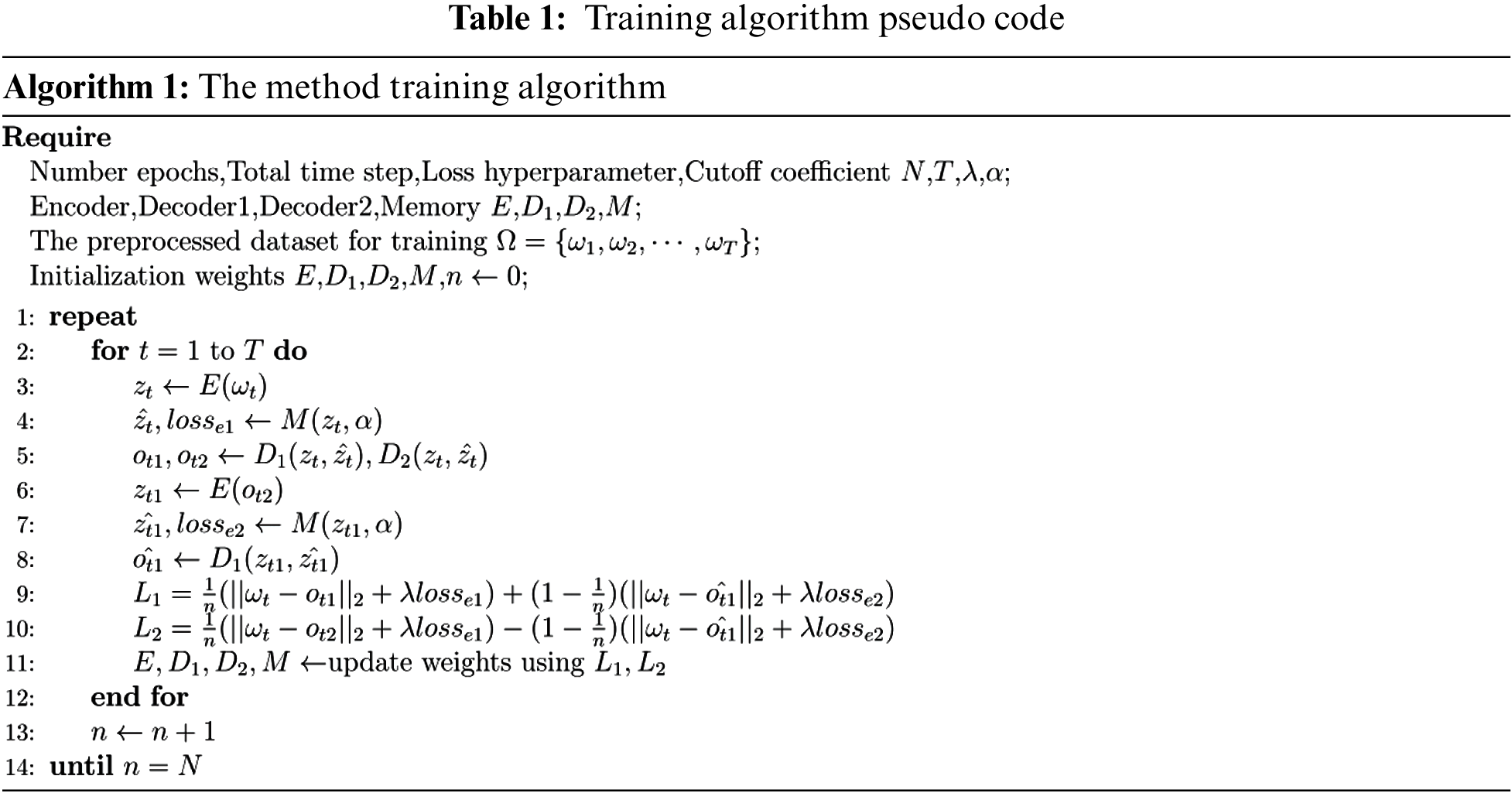
The encoder training phase aims to train the deep memory autoencoder structure to reconstruct normal samples, as indicated by the blue line in Fig. 1. This research uses the reconstruction error of each depth autoencoder as the first part of the training loss function. In addition, to make the feature vector consist of only a few closest memory units [31], this research uses losse1 that the entropy of w^ as the second part of the training loss function. losse1 and the loss functions of the two autoencoders at this stage are shown in Eqs. (11)–(12).

losse1=∑i=1N−w^i⋅log⁡(w^i)(11)

L1=||Ω−O1||2+losse1L2=||Ω−O2||2+losse1(12)

The adversarial training phase aims to train autoencoder1 to distinguish between the real data and the reconstructed data from autoencoder2 and to train autoencoder2 to fool autoencoder1. The yellow line shows the process in Fig. 1, where the reconstructed data O2 from autoencoder2 is used as input to autoencoder1, and the reconstructed data O^1 is obtained. The loss function of this part is shown in Eq. (13).

minDecoder1maxDecoder2(||Ω−O^1||2+losse2)(13)

For training purposes, we rewrite this loss in the following Eqs. (14) and (15).

L1=||Ω−O^1||2+losse2(14)

L2=−||Ω−O^1||2−losse2(15)

The loss function of the two autoencoders during our train is shown in Eqs. (16) and (17).

L1=1n(||Ω−O1||2+λlosse1)+(1−1n)(||Ω−O^1||2+λlosse2)(16)

L2=1n(||Ω−O2||2+λlosse1)−(1−1n)(||Ω−O^1||2+λlosse2)(17)

where n is the number of training epochs and λ is the hyperparameter for reconciling reconstruction error and the entropy of w^.

3.3.3 Abnormal Inference Process

In the abnormal inference process, this research inputs the test dataset samples to the trained model to obtain the reconstruction samples and calculate the reconstruction error. Finally, the POT method determines the threshold value to distinguish between abnormal and normal samples. The pseudo-code of the abnormal inference process is shown in Table 2.

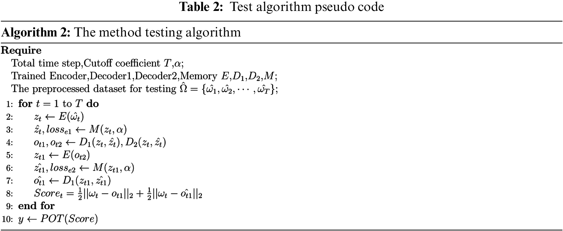
In the anomaly inference stage, this research uses the average reconstruction error of the original input and the reconstructed input of autoencoder1 and autoencoder2 as the score for judging anomalies, as shown in Eq. (18).

Score=12||Ω−O1||2+12||Ω−O^1||2(18)

This research uses the POT method to determine the threshold value automatically, and abnormal scores exceeding the threshold value are judged as abnormal samples and vice versa, as shown in Eq. (19).

yi={1,if Scorei>POT(Score)0,otherwise(19)

4  Experiments and Results

4.1 Datasets

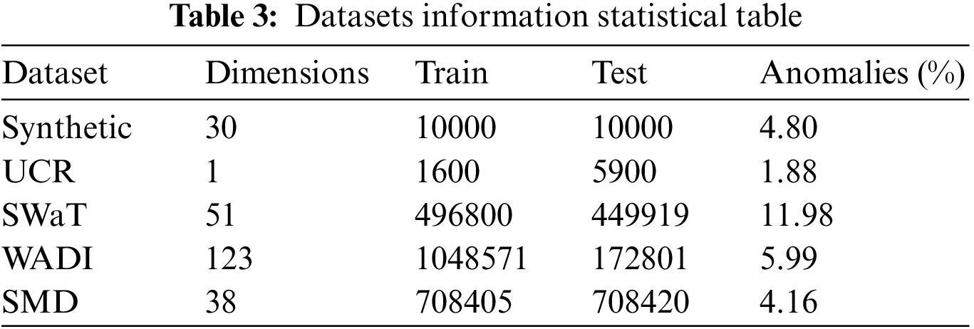
This research uses a synthetic dataset and four datasets from power systems, water treatment plants, and computer clusters to validate the effectiveness of our proposed method [32–35]. We count the information of these datasets, including data volume, dimensionality, and anomaly percentage, as shown in Table 3.

•   Synthetic: This study uses the synthetic dataset proposed in [32], which uses sin and cos to simulate time series with randomly selected time delays and frequencies within a certain range. Finally, five random artificially created anomalies are added.

•   UCR: This dataset is provided by the Knowledge Discovery and Data (KDD) 2021 competition [33], and this research selects the internal bleeding and egg datasets from the real world.

•   SWaT: This dataset is collected from data generated by sensors in real water treatment plants, and it contains seven days of normal operation and four days of abnormal data [34].

•   WADI: This dataset is collected from the sensors data [34] but contains more sensors and attack scenarios than SWaT.

•   SMD: This dataset is collected from 28 computer resource utilization data [35], and this study focuses only on non-trivial sequences in the dataset, specifically machine-1-1, 2-1, 3-2, and 3-7. This research is consistent with [29] in selecting and preprocessing these datasets.

4.2 Evaluation Indicators

This research evaluates model performance based on four metrics: Precision, Recall, Area Under Curve (AUC), and F1 score. Where Precision and Recall are calculated from True positive (TP), False Negative (FN), False Positive (FP), and True Negative (FN), AUC is the area under the Receiver Operating Characteristic (ROC) curve. The F1 score is calculated from Precision and Recall metrics, as shown in Eq. (20).

F1−score=2∗Precision∗RecallPrecision+Recall(20)

4.3 Contrast Methods and Parameter Environment Settings

This research compares the proposed method with various advanced methods proposed in recent years, including Merlin [21], LSTM-NDT [22], DAGMM [24], USAD [2], CAE-M [25], GDN [27], and TranAD [29]. Merlin is a parameter-free method, and this research compares it as an example of a statistical-based method. LSTM-NDT uses the LSTM structure and NDT, and this research compares it as an LSTM-based method. DAGMM is a method that combines autoencoder and parameter estimation. In this study, DAGMM is considered a representative method of the autoencoder-based method for comparison experiments. USAD uses adversarial training for the first time for time series anomaly detection, so we treat it as a comparison method. CAE-M applies CNN to information extraction and is considered a representative method of the CNN-based approach for comparison experiments. GDN is a method of constructing data into a graph structure and is considered a representative method of the graph-based approach for comparison experiments. Moreover, TranAD is a method that applies transformers to time series anomaly detection and is considered a representative method of the transformer-based method for comparison experiments. The results of the contrastive methods are referred to as the reproduction work of TranAD.

This experiment chooses the AdamW optimizer to train the model, set the initial learning rate to 0.01, and the step scheduler to 0.5. This experiment chooses the window size with the best results among [5, 10, 20, 50, 100], the number of layers of autoencoder to 3, the length of the feature vector to 10, the number of memory cells to 20, the truncation parameter to the 20th quantile of the similarity vector, the loss function to 0.1, and the parameters in POT to 10e-4. All the above model parameters are determined by grid search. The experimental environment uses Windows 10 operating system. The main hardware parameters are: the Central Processing Unit (CPU) uses Intel(R) Core(TM) i7-9750H CPU @ 2.60 GHz, the Graphics Processing Unit (GPU) uses an NVIDIA GeForce RTX 2060 with 6G dedicated memory, the programming language uses Python 3.8, and the model structure is built using Pytorch 1.8.0.

4.4 Anomaly Detection Results

In order to prove that our proposed method is effective, this research does anomaly detection experiments on five datasets with seven comparison methods, and the experimental results are shown in Table 4. It can be seen from the results that our proposed method performs well on almost all datasets.

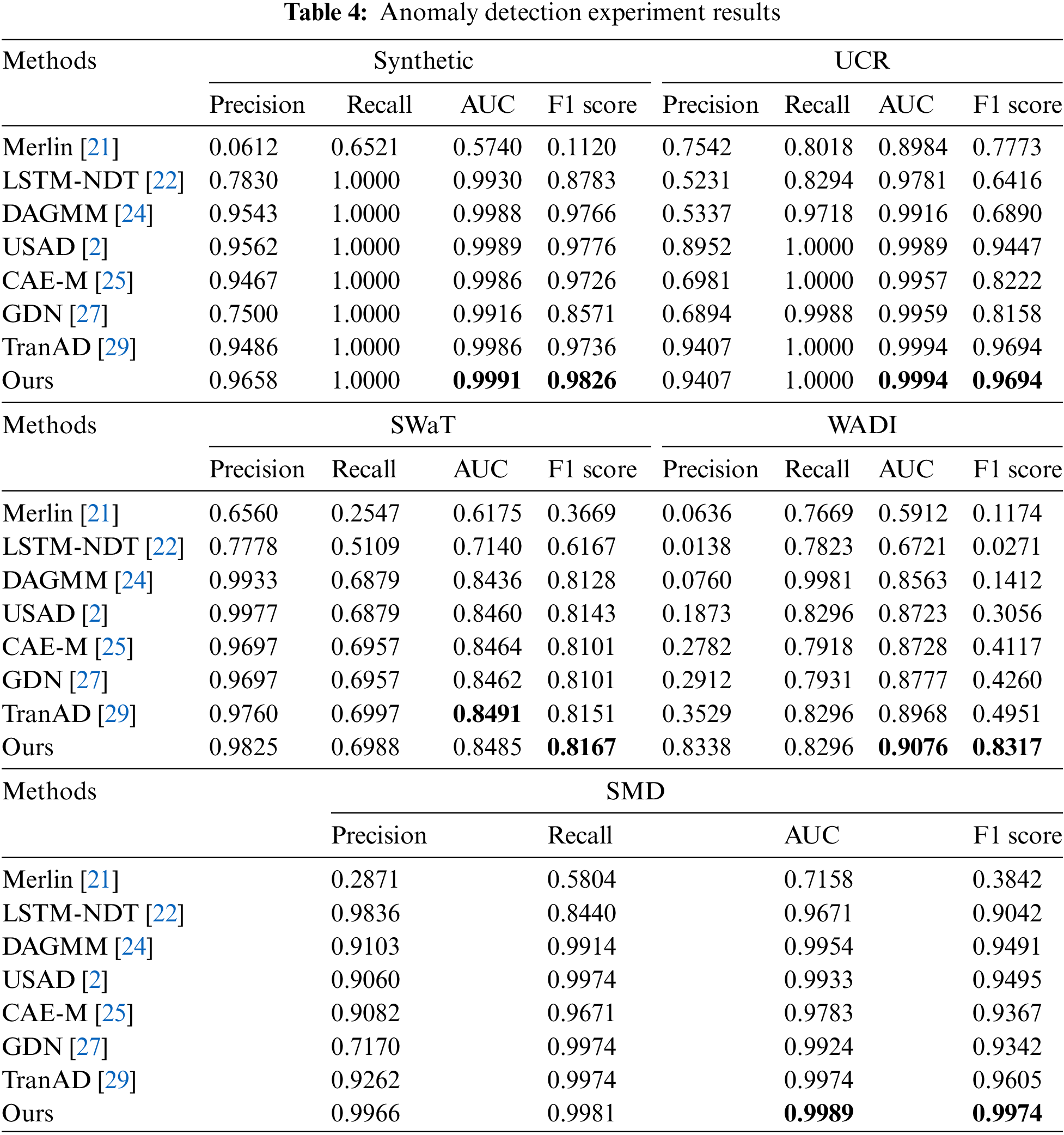
The experimental results show that Merlin, as a traditional statistical machine learning method, cannot capture the relationship between different features in the data, resulting in poor performance on multivariate time series. LSTM-NDT performs better on the SMD dataset due to fully considering the time dependence. However, the method of determining the threshold by NDT is poorly adaptable to different scenarios, so it performs poorly on the other four datasets [27]. Our proposed method can obtain more accurate thresholds by using local peaks in the sequence through the POT method. DAGMM performs well on Synthetic, SWaT, and SMD datasets due to parameter estimation on high dimensional data. However, due to its inability to capture data relationships in different dimensions, it performs poorly on the other two datasets. Our proposed method slices high dimensional data by sliding window operation and extracts the information in different dimensions using fully connected layers. USAD achieves good results on all five datasets, illustrating the suitability of the adversarial training strategy for anomaly detection work in time series. Therefore, our proposed method also includes the strategy of adversarial training. CAE-M uses sequential observations as input to perform reconstruction without considering anomalous data, which can help them detect anomalies close to normal trends. However, it uses CNN and LSTM simultaneously, resulting in excessive resource consumption. Our proposed method uses a memory module to record the prototype patterns of normal samples, which can detect anomalous samples close to normal samples with fewer resources. GDN and TranAD are relatively novel approaches proposed recently. They use the relationship between different features in the data and the longer time dependence to obtain very good detection results. However, they do not restrain the overgeneralization of the model, and there is a gap between the anomaly detection performance and the proposed method.

Our proposed method achieves the best results on all five datasets. The AUC average reached 0.9507, and the F1 score average reached 0.9196. The improvement is smaller on Synthetic, UCR, and SWaT datasets. The Synthetic dataset contains only the more obvious anomalies injected by hand, and good detection results can be obtained by autoencoder alone. The UCR dataset contains few anomalous samples, resulting in minor model enhancement. The reconstruction method cannot detect some anomalies in the SWaT dataset, so the effect improvement is not obvious. Even so, the results on these three datasets show the effectiveness of our proposed method for general anomalies. The effect is significantly improved on the WADI dataset and the SMD dataset. In comparison to the TranAD method, our proposed method improves F1 score metric performance by 34% on the WADI dataset and 3.7% on the SMD dataset due to the use of a memory module to record normal samples with prototype patterns and the ability to forget partial feature information to restrain model overgeneralization. This research analyzes the model’s significant effect improvement on the WADI dataset in Section 4.6.

4.5 Ablation Experiments

This research designs ablation experiments to illustrate how each component of the proposed method affects the model’s performance. This research compares the conventional autoencoder, the autoencoder with the addition of adversarial training, and the autoencoder with the addition of the memory module. The experimental results are shown in Table 5.

The experimental results show that adding adversarial training creates a higher precision rate on the Synthetic and UCR datasets. In contrast, the recall rate remains unchanged, indicating that adding adversarial training can further widen the reconstruction error gap. The addition of the memory module alone increases recall and F1 score. It decreases FN while maintaining no decrease in precision on the SWaT, WADI, and SMD datasets, indicating that the memory module restrains the overgeneralization of the model and detects some abnormal data that are close to normal. However, by adding adversarial training alone, the precision becomes lower in the SMD dataset due to stretching the reconstruction error of some normal samples. The inclusion of the memory module alone decreased precision on the Synthetic dataset, indicating that the inclusion of two modules alone may lead to model instability. Adding two modules yield more effective and stable results than adding one module alone on all five datasets.

4.6 Results Analysis

In order to illustrate in detail how our proposed method works, this research compares the results of the ablation experiments on the WADI dataset, as shown in Fig. 2. We classify points with reconstruction errors larger than the threshold as abnormal and those with reconstruction errors less than normal. The result divides the real normal samples into four categories: blue, green, yellow, and black. This research finds several phenomena and gives explanations for the reasons behind these phenomena.

•   Observation 1: After adding adversarial training alone, it still discriminates many normal samples as anomalous samples, and the improvement in anomaly detection performance is not obvious.

•   Analysis: The adversarial training can stretch the reconstruction error further if it is large (expanding the largest reconstruction error from 16 to 28). Still, this approach does not significantly improve the detection performance if the reconstruction error of the anomalous samples obtained by the autoencoder method is already small. (Improvement is only observed for some green and purple regions)

•   Observation 2: After adding the memory module alone, the anomalies’ reconstruction error exceeds most normal samples’ reconstruction error.

•   Analysis: The memory unit records prototype patterns of the data. It allows some information to be forgotten in reconstructing the samples to restrain overgeneralization of the model, causing the reconstruction error to become larger for abnormal samples close to normal samples (the average reconstruction error for abnormal samples changes from 8.06 to 10). The increased reconstruction error of the anomalous samples leads to a substantial improvement in anomaly detection performance (the reconstruction error of the anomalous samples already exceeds the reconstruction error of the normal samples represented by the green, purple, and most of the yellow regions). However, some may enlarge the reconstruction error of normal samples (the reconstruction error of normal samples becomes larger in some blue regions).

•   Observation 3: By adding the memory module and adversarial training, the reconstruction error of the abnormal samples is clearly distinguished from that of most normal samples.

•   Analysis: Since the reconstruction error of the anomalous samples obtained by adding the memory module is large enough, adding the adversarial training can make this part of the reconstruction error larger again (the average reconstruction error of the anomalous data changes from 10 to 18.68). It makes the abnormal samples distinguishable from more normal samples (some normal samples are represented by the blue regions).

Figure 2: Ablation experiment results on the WADI dataset

4.7 Sensitivity Analysis

In order to explore the influence of the sliding window size on the model results, this research designs a sensitivity analysis experiment, as shown in Fig. 3. If the sliding window is too small, the local information representation is insufficient, which will cause the model to fail to achieve good results. If the sliding window is too large, some local anomalies will be ignored, resulting in decreased model performance.

Figure 3: F1 score and ROC/AUC score with window size

4.8 Complexity Analysis

This research designs the complexity analysis experiments. The results are shown in Table 6, which uses the time spent to train each epoch to represent the complexity of the model. This study introduces the memory module and adversarial training in a way that leads to the high complexity of the model. Introducing parallel structures, such as transformers, is our future research direction to solve the high complexity.

5  Conclusions

This research proposes a new anomaly detection method for multivariate time series based on a deep memory autoencoder. Firstly, a memory module is introduced to record the feature vectors’ prototype information to suppress the model’s overgeneralization, which can identify abnormal samples close to the normal ones. Secondly, this research trains the model in adversarial training to expand the reconstruction difference between normal and abnormal samples, making our model more stable. Finally, thresholds for normal and abnormal samples are automatically determined using the POT method, eliminating the need to find specific thresholds for each dataset. This research validates the effectiveness of the proposed method on Synthetic and four real-world datasets. The results show that our method has excellent detection ability in almost all datasets compared with seven existing methods. Our method can improve the AUC and F1 score metrics compared with the suboptimal method model, up to 8% and 33.6%. Ablation experiments illustrate that both parts of the model are effective and necessary, and the analysis of the results explains in detail how our proposed method improves anomaly detection performance. However, we discover that the model’s execution time is slightly slower than the average time of the comparison models, placing it sixth out of seven methods in terms of execution time. Reducing model complexity and improving model efficiency are the directions for future improvement.

Funding Statement: This research is supported by the National Natural Science Foundation of China (62203431)

Conflicts of Interest: The authors declare that they have no conflicts of interest to report regarding the present study.

References

1. G. Jonathan, A. Sridhar, T. Marcus and S. L. Zi, “Anomaly detection in cyber physical systems using recurrent neural networks,” in IEEE 18th Int. Symp. on High Assurance Systems Engineering (HASE), Singapore, pp. 140–145, 2017. [Google Scholar]

2. L. Dan, C. Dacheng, S. Lei, J. Baihong, G. Jonathan et al., “MAD-GAN: Multivariate anomaly detection for time series data with generative adversarial networks,” in 28th Int. Conf. on Artificial Neural Networks (ICANN), Munich, Germany, pp. 703–716, 2019. [Google Scholar]

3. W. Z. Yi and H. Y. Kun, “Time series data decomposition-based anomaly detection and evaluation framework for operational management of smart water grid,” Journal of Water Resources Planning and Management, vol. 147, no. 9, pp. 76–95, 2021. [Google Scholar]

4. R. K. A., I. M. Tahir, S. Abdeslam and A. W. S, “Wavelet based detection of outliers in volatility time series sodels,” Computers Materials & Continua, vol. 72, no. 2, pp. 3835–3847, 2022. [Google Scholar]

5. G. E. P. Box and D. A. Pierce, “Distribution of residual autocorrelations in autoregressive-integrated moving average time series models,” Journal of the American Statistical Association, vol. 65, no. 332, pp. 1509–1526, 1970. [Google Scholar]

6. B. Schölkopf, R. C. Williamson, A. Smola, J. S. Taylor and J. Platt, “Support vector method for novelty detection,” in 13th Annual Conf. on Neural Information Processing Systems (NIPS), Denver, CO, USA, pp. 582–588, 2000. [Google Scholar]

7. M. M. Breunig, H. P. Kriegel, R. T. Ng and J. Sander, “LOF: Identifying density-based local outliers,” in Int. Conf. on Management of Data, Dallas, TX, USA, pp. 93–104, 2000. [Google Scholar]

8. G. A. Wilkin and X. Huang, “K-means clustering algorithms: Implementation and comparison,” in Second Int. Multi-Symp. on Computer and Computational Sciences (IMSCCS), Iowa City, IA, USA, pp. 133–136, 2007. [Google Scholar]

9. A. Blázquez-García, A. Conde, U. Mori and J. A. Lozano, “A review on outlier/anomaly detection in time series data,” ACM Computing Surveys, vol. 54, no. 3, pp. 1–31, 2022. [Google Scholar]

10. T. Amarbayasgalan, V. H. Pham, N. T. Umpon and K. H. Ryu, “Unsupervised anomaly detection approach for time-series in multi-domains using deep reconstruction error,” Symmetry, vol. 12, no. 8, pp. 1251–1273, 2020. [Google Scholar]

11. A. Siffer, P. A. Fouque, A. Termier and Largouet C., “Anomaly detection in streams with extreme value theory,” in 23rd ACM SIGKDD Int. Conf. on Knowledge Discovery and Data Mining, Halifax, Canada, pp. 1067–1075, 2017. [Google Scholar]

12. M. D. Nadai and M. V. Someren, “Short-term anomaly detection in gas consumption through ARIMA and artificial neural network forecast,” in 2015 IEEE Workshop on Environmental, Energy, and Structural Monitoring Systems (EESMS), Trento, Italy, pp. 250–255, 2015. [Google Scholar]

13. V. Kozitsin, I. Katser and D. Lakontsev, “Online forecasting and anomaly detection based on the ARIMA model,” Applied Sciences, vol. 11, no. 7, pp. 3194–3207, 2021. [Google Scholar]

14. B., Lamrini, A. Gjini, S. Daudin, P. Pratmarty, F. Armando et al., “Anomaly detection using similarity-based one-class SVM for network traffic characterization,” in 29th Int. Workshop on Principles of Diagnosis, Warsaw, Poland, pp. 178–193, 2018. [Google Scholar]

15. S. D. D. Anton, S. Sinha and H. Dieter Schotten, “Anomaly-based intrusion detection in industrial data with SVM and random forests,” in 27th Int. Conf. on Software, Telecommunications and Computer Networks (SoftCOM), Split, Croatia, pp. 1–6, 2019. [Google Scholar]

16. H. Z. You, X. X. Lei and D. S. Chun, “Discovering cluster-based local outliers,” Pattern Recognition Letters, vol. 24, no. 9–10, pp. 1641–1650, 2003. [Google Scholar]

17. W. Fang, W. Zhe and Z. Xu, “Anomaly IoT node detection based on local outlier factor and time series,” Computers Materials & Continua, vol. 64, no. 2, pp. 1063–1073, 2020. [Google Scholar]

18. S. Chawla and A. Gionis, “K-means–: A unified approach to clustering and outlier detection,” in Proc. of the 2013 SIAM Int. Conf. on Data Mining, Austin, TX, USA, pp. 189–197, 2013. [Google Scholar]

19. M. Goldstein and S. Uchida, “A comparative evaluation of unsupervised anomaly detection algorithms for multivariate data,” Plos One, vol. 11, no. 4, pp. e0152713, 2016. [Google Scholar]

20. L. J. Bo, W. Pedrycz and I. Jamal, “Multivariate time series anomaly detection: A framework of hidden markov models,” Applied Soft Computing, vol. 60, pp. 229–240, 2017. [Google Scholar]

21. T. Nakamura, M. Imamura, R. Mercer and E. Keogh, “MERLIN: Parameter-free discovery of arbitrary length anomalies in massive time series archives,” in 20th IEEE Int. Conf. on Data Mining (ICDM), Sorrento, Italy, pp. 1190–1195, 2020. [Google Scholar]

22. T. Soderstrom, I. Colwell, C. Laporte, V. Constantinou and K. Hundman, “Detecting spacecraft anomalies using LSTMs and nonparametric dynamic thresholding,” in 24th ACM SIGKDD Conf. on Knowledge Discovery and Data Mining (KDD), London, England, pp. 387–395, 2018. [Google Scholar]

23. P. Malhotra, A. Ramakrishnan, G. Anand, L. Vig, P. Agarwal et al., “LSTM-Based encoder-decoder for multi-sensor anomaly detection,” arXiv e-prints, arXiv: 1607.00148, 2016. [Google Scholar]

24. Z. Bo, S. Qi, M. R. Min, C. Wei, C. Lumezanu et al., “Deep autoencoding gaussian mixture model for unsupervised anomaly detection,” in 2018 Int. Conf. on Learning Representations (ICLR), Vancouver, BC, Canada, pp. 89–95, 2018. [Google Scholar]

25. Y. Zhang, Y. Chen, J. Wang and Z. Pan, “Unsupervised deep anomaly detection for multi-sensor time-series signals,” IEEE Transactions on Knowledge and Data Engineering, vol. 35, no. 2, pp. 2118–2132, 2021. [Google Scholar]

26. J. Audibert, P. Michiardi, F. Guyard, S. Marti and M. A. Zuluaga, “Usad: Unsupervised anomaly detection on multivariate time series,” in 26th ACM SIGKDD Int. Conf. on Knowledge Discovery and Data Mining (KDD), San Diego, CA, USA, pp. 3395–3404, 2020. [Google Scholar]

27. A. Deng and B. Hooi, “Graph neural network-based anomaly detection in multivariate time series,” in 35th AAAI Conf. on Artificial Intelligence (AAAI), Vancouver, BC, Canada, pp. 4027–4035, 2021. [Google Scholar]

28. H. Zhao, Y. Wang, J. Duan, C. Huang, D. Cao et al., “Multivariate time-series anomaly detection via graph attention network,” in 20th IEEE Int. Conf. on Data Mining (ICDM), Sorrento, Italy, pp. 841–850, 2020. [Google Scholar]

29. S. Tuli, G. Casale and N. R. Jennings, “TranAD: Deep transformer networks for anomaly detection in multivariate time series data,” arXiv preprint, arXiv:220107284, 2022. [Google Scholar]

30. Z. Chen, D. Chen, X. Zhang, Z. Yuan and X. Cheng, “Learning graph structures with transformer for multivariate time-series anomaly detection in IoT,” IEEE Internet of Things Journal, vol. 9, no. 12, pp. 9179–9189, 2021. [Google Scholar]

31. D. Gong, L. Liu, V. Le, B. Saha, M. R. Mansour et al., “Memorizing normality to detect anomaly: Memory-augmented deep autoencoder for unsupervised anomaly detection,” in 2019 IEEE/CVF Int. Conf. on Computer Vision (ICCV), Seoul, South Korea, pp. 1705–1714, 2019. [Google Scholar]

32. C. Zhang, D. Song, Y. Chen, X. Feng, C. Lumezanu et al., “A deep neural network for unsupervised anomaly detection and diagnosis in multivariate time series data,” in Proc. of the AAAI Conf. on Artificial Intelligence (AAAI), Honolulu, HI, USA, pp. 1409–1416, 2019. [Google Scholar]

33. E. Keogh, D. R. Taposh, U. Naik and A. Agrawal, “Multi-dataset time-series anomaly detection competition,” in 27th ACM SIGKDD Conf. on Knowledge Discovery and Data Mining, Singapore, pp. 201–216, 2021. [Google Scholar]

34. A. P. Mathur and N. O. Tippenhauer, “SWaT: A water treatment testbed for research and training on ICS security,” in 2016 Int. Workshop on Cyber-Physical Systems for Smart Water Networks (CySWater), Vienna, Austria, pp. 31–36, 2016. [Google Scholar]

35. S. Ya, Z. Y. Jian, N. C. Hao, L. Rong, S. Wei et al., “Robust anomaly detection for multivariate time series through stochastic recurrent neural network,” in 25th ACM SIGKDD Int. Conf. on Knowledge Discovery & Data Mining (KDD), Anchorage, AK, USA, pp. 2828–2837, 2019. [Google Scholar]