Alzheimer’s Disease Stage Classification Using a Deep Transfer Learning and Sparse Auto Encoder Method

1  Introduction

Alzheimer’s Disease (AD) is the most debilitating brain disease affecting any age, especially the elderly. A condition undertreated and under-recognized is becoming a serious public health concern. Alzheimer’s Disease (AD) is a significant public health problem impacting life expectancy. AD was first identified in 1906 by Alois Alzheimer, who employed memory loss, pathology indications, and disorientation as diagnostic criteria [1]. AD can express itself clinically, including memory, language, visuospatial, and executive function impairments. Personality changes, impaired judgement, aimlessness, insanity, agitation, sleep difficulties, and mood disturbances are examples of behavioural and non-cognitive symptoms [2]. Brain alterations linked to the development of Alzheimer’s Disease may begin two decades or more before any manifestations of the disease are evident, according to scientists [3]. The different phases of the disease are named: Intellectually Ordinary or Cognitively Normal (CN), Mild Cognitive Impairment (MCI), Early Mild Cognitive Impairment (EMCI), Late Mild Cognitive Impairment (LMCI) and Alzheimer’s Disease (AD). CN subjects typically indicate maturing with no traces of sadness and dementia [4]. MCI patients are more prone to experience an early onset of Alzheimer’s disease. Imaging biomarkers are considered one of the robust identification tools to diagnose the early phases of Alzheimer’s Disease [5], such as Magnetic Resonance Imaging (MRI), Functional MRI (fMRI), and Positron Emission Tomography (PET). Fig. 1 depicts the different stages of MCI to AD with MRI.

Figure 1: Classification stages as (a) Mild Cognitive Impairment (MCI), (b) Early MCI (EMCI), (c) Late MCI (LMCI), and (d) Alzheimer’s Disease (AD). The blue marker line represents the shrinking of the brain and the red markers show the enlarged ventricles as the disease advances

MCI, EMCI and LMCI are the significant stages before stepping into AD, in which the sickness has progressed and started to impede ordinary or daily life activities. The patient displays side effects, including loss of motor coordination, discourse issues, memory issues, and inability to peruse and compose. Neuropsychological tests are utilized to recognize the seriousness of MCI. AD addresses the high-level and deadly phase of the sickness [6,7]. There seems to be no comprehensive treatment for curing AD completely; however, the correct medicine and sufficient care can aid patients’ quality of life. In the beginning phases of Alzheimer’s infection, mental misfortune or cognitive instability can be ended, regardless of the incurable AD [8,9]. Therefore, an early and timely AD diagnosis is essential to improve and provide a beneficial quality to patients’ lives.

Deep Learning (DL) has demonstrated enormous possibilities for clinical support in deciding on several diseases, including diabetic retinopathy, malignancies, and Alzheimer’s Disease (for imaging investigation) [10]. The essential benefit of Deep learning over traditional shallow learning models is its capacity to gain the best prescient qualities for prediction and classification straightforwardly from unlabeled information [11,12]. It uses Graphics Processing Units (GPUs) that have become more potent as computing power has increased, allowing for the creation of competitive and leading-edge deep learning models and algorithms [13]. Deep Learning (DL) mimics the functioning of the neural network in a human brain, processes the data, and identifies the pattern formation to handle complex decision-concerning problems [14,15]. DL can understand pattern formation and is capable enough to make a conclusion for optimization problems [16,17]. In particular, Convolutional Neural Networks (CNNs) have recently achieved marvelous success in the medical field for segmenting regions and identifying disorders [18]. DL methods may be used to detect hidden interpretations in neuroimaging data, as well as to establish connections between various portions of imagery and identify patterns associated with the disease. MRI, fMRI, PET, and Diffusion Tensor Imaging (DTI) are examples of medical imagery where DL models have been effectively deployed. Researchers have recently started exhaustively utilizing computer vision and DL models to identify brain disorders from various medical images; however, the DL can be utilized with both medical images and clinical parameters in diagnosing and classifying AD. DL also has applications in domains like object detection, contextual analysis, disaster management, person Re-ID, and vehicle Re-ID [19]. Some of the most representative metaheuristic algorithms, like monarch butterfly optimization (MBO), earthworm optimization algorithm (EWA), elephant herding optimization (EHO), and moth search (MS) algorithm, are used in large-scale optimization problems, especially in health care research [20].

This work aimed to develop a framework for feature extraction, reduction and multi-class classification of AD using pre-trained models of CNN, sparse autoencoders and a Deep Neural Network (DNN).

The overlapping characteristics of Alzheimer’s Disease make it difficult to classify its distinct stages. Most of the published research focuses on binary classification. The classification of two or more phases of this illness requires in-depth effort. This research aims to do a multi-class categorization of the 5 AD phases comprising CN, MCI, EMCI, LMCI and AD.

The format of the paper is described as follows: Section 2 depicts the literature survey, Section 3 encloses datasets, and Section 4 explains the methodology. It describes the preprocessing, feature extraction model and classification model. Section 5 gives a view of performance metrics. Section 6 represents the results and their analysis, and the paper complete with Section 7 of the conclusion.

2  Background Study

This section reviews recent approaches to classifying AD and MCI using computer-aided design models and algorithms. A volumetric convolutional neural network (CNN)-based research has been developed for AD detection and classification in the paper [21]. The normal control and AD MRI images were pre-trained with a convolutional autoencoder. This was followed by supervised learning using the task-specific tuning approach to construct a classifier capable of distinguishing AD from NC. The MCI classification is more strenuous than AD categorization with normal control. In the transfer learning technique, learning is done as two or more tasks. The visual representation acquired or weights learnt from NC vs. AD are transferred to the categorization of progressive MCI (pMCI) vs. stable MCI (sMCI). For AD detection, the paper [22] aimed at a Content-Based Image Retrieval (CBIR)-based system with 3D-CNN and pre-trained 3D-autoencoder technology Capsule Network. The technique uses a 3D sparse for feature extraction from MRI, a query-based image retrieval system and a 3D CNN for classification. The Capsule Network uses fewer datasets than a typical CNN, is capable of rapid learning, and efficiently handles image rotations and transitions. The effort primarily focuses on determining how well the system can capture the attributes for enhanced CBIR performance. The algorithm is efficient, straightforward, and well-suited for modest computational resources. The system displays binary classifications for MCI vs. AD, NC vs. AD, MCI vs. AD, and NC vs. AD.

A classifier for AD and its evolution by merging CNN and EL (Ensemble Learning) was introduced in [23]. The EL algorithm generates a series of base classifiers; with the provided data set, it discriminates characteristics to offer a weighted note per class. Several baseline classifiers were trained using unique 2D MRI slices and the CNN approach. The research focused on the binary classifications of AD or MCI Convert (MCIc) vs. HC and MCIc vs. MCI does not convert (MCInc). The paper focused on modelling multimodality CNN-based classifiers only for AD diagnosis and prognosis. The research [24,25] highlighted the disease classification from MCI to AD using images and protein level counts such as, fluorodeoxyglucose (FDG), positron emission tomography (PET), MRI, Cerebro Spinal Fluid (CSF) protein levels, and the apolipoprotein E (APOE) genotype. A novel kernel-based multiclass SVM classifier was used for the classification. The paper [26] focused on an autoencoder 3D CNN and 2D CNN to sort the cerebral images. Accuracy rates of 85.53% for 3D CNN models and 88.53% for 2D CNN models were achieved. The literature review [27] utilized MRI and fMRI images to distinguish Alzheimer’s patients from healthy control participants. For binary classification, LeNet-5 and Google Net have been employed as network designs.

The existing approaches focused on the binary classification of AD, MCI and their variations. Though the significant factor of AD is its age criteria, the classification based on young onset and later onset categories wasn’t carried out. The proposed method focused on the young-onset group, as it’s difficult to detect and classify. But working on this age group helps the practitioner as a support system in finding and classifying AD and increasing their life expectancy. This research work contributed to the following areas, which helped to address the inadequacies of the existing work.

•   The proposed work is to find and label the early stages of AD in both men and women between the ages of 45 and 65 who get it at a young age.

•   The subject selection for the current work is not only based on age but also on their clinical test and gene protein values.

•   A Contrast Limited Adaptive Histogram Equalization method was used on the selected sagittal MRIs of the subjects to get the best values for improving the images without losing fine details.

•   As part of the current work, a deep transfer learning model with a sparse autoencoder and a neural network for detection and classification is being designed in five steps.

•   In the current work, the hyper-parameters of the deep neural network model are tuned to attain an accuracy level of 95% to 100%.

3  Neuroimaging Dataset

Alzheimer’s Disease Neuroimaging Initiative (ADNI) is a multi-institutional research database that provides biomarkers for AD detection and classification. It includes genetic, biochemical, neuroimaging and clinical biomarkers and can help identify and track AD and its prognosis. Neuroimaging contains multi modalities such as PET, MRI, fMRI and DTI. All images presented in the proposed paper were obtained from the ADNI repository, which can be found at https://www.loni.ucla.edu/ADNI and https://www.adni-info.org. The proposed research has used the 3D MRI neuroimaging modality as the indicator. The dataset contains MRIs of 325 patients of both gender, 168 males and 157 females of the age category of 45 to 65 years. Each subject had 166 MRI slices from the left side of the brain to the right side, with a voxel volume of 1.5 mm, taken over five years of monitoring every three to six months. The categories considered for the current work are Control Normal, Mild Cognitive Impairment, Early-MCI, Late-MCI and Alzheimer’s Disease. From each category, a set of 1200 images collected for the proposed work. The dataset offers essential information on the cognitively normal, MCI and AD subjects. The individuals are diagnosed and labelled as the stages from MCI to AD based on the results of neuroimaging and clinical biomarkers such as, Mini-Mental State Examination (MMSE), Clinical Dementia Rate (CDR), Frequently Asked Questions (FAQ), Neuropsychiatric Inventory Questionnaire (NPI-Q) and gene protein value Apolipo Protein-E (APOE).

4  Methodology

The proposed methodology entrusts with detecting and classifying Mild Cognitive Impairment in the Alzheimer’s Disease stage. It can achieve in three steps, which are as follows: (1) image preprocessing, (2) feature extraction and size reduction using transfer learning models and sparse autoencoder, (3) A fine-tuned neural network’s multi-class classification of disease stage. Fig. 2 describes the framework of the proposed system.

Figure 2: Proposed model for AD classification

4.1 Preprocessing

In image processing, intensity normalization is a technique of modifying the spectrum of pixel intensity values, sometimes referred to as histogram stretching or contrast stretching. This method intends to put the image into a range that is more natural or recognizable to the senses. The proposed work encompasses the adaptive Weiner filter and histogram equalization methods for noise removal and image enhancement. Applied a median filter, an adaptive median filter, and an adaptive Weiner filter to the given input image. The Weiner filter is considered for the work, as it shows less error when calculated through Peak Signal-to-Noise Ratio (PSNR) [28]. The Weiner filter is one of the most prevalent and widely employed nonlinear filters, and its smoothening procedure lowers the noise of the input image [29]. This filter also reduces the intensity difference between pixels in an MRI [30]. For filtering, a 3 × 3 window size has been used, as this is an appropriate window size for image filtering in the current work.

X(i,j)=W(Y(i,j),[m,n])(1)

where Y(i,j), is the noisy input image, W is the Weiner function and [m,n] is the window size of the neighbourhood cells to calculate the standard deviation and mean. The filtered output image is stored in X(i,j). Contrast Limited Adaptive Histogram Equalization (CLAHE) was applied to the noise-free image for additional enhancement. It solves the problem of histogram equalization (HE) over-amplification by reducing noise in homogenous zones [31]. CLAHE highlights the hidden and finer details of the image and maintains the level of contrast while enhancing the image. CLAHE utilized a clip point to regulate and restrict the contrast level obtained by traditional HE.CLAHE divides the image into tiles of height and width pixels and also divides the image into non-overlapping blocks [32]. In MRI, the CLAHE operates on tiles, which are tiny patches. In addition, it generates several histograms and evaluates each to a certain image region. CLAHE can adjust the contrast or brightness of an image [33].

A(i,j)=Ad(X(i,j),NT(m,n),CL(cl)(2)

The input image is X(i,j), the CLAHE function is Ad and it enhances the contrast based on the number of tiles and clip limit considered for the given images. NT(m,n) represents the number of images divided into tiles as rows and columns. CL (cl) sets the threshold to limit the contrast. The enhanced output images are stored in the A(i,j). The Fig. 3 represents original and processed images with the filtering techniques.

Figure 3: Represents the original and processed where (a)–(e): are original images of the AD, CN, MCI, EMCI and LMCI respectively. The (f)–(j) images are preprocessed with an adaptive weiner filter and CLAHE equalization for the corresponding (a)–(e) original images

4.2 Feature Extraction and Dimensionality Reduction

The primary purpose of feature extraction is to identify the most salient data that may be utilized for data representation, high-dimensional data categorization, visualization and storage. In this section, the feature extraction is carried out with pre-trained CNN models and forwarded to the stacked autoencoder for dimensionality reduction. This strategy could extract an enlarged number of features from the selected datasets of ADNI. The preprocessed input data has been forwarded to the selected five transfer learning models such as Resnet-18, Inception-v3, Googlelenet, Alexnet and VGG-16. The input image is scaled under the specified size needed by the models before being fed into the network. However, the number of images currently available is 6000 (1200 × 5) for all the classes. It is considered a limited count to provide an optimum classification to avoid this scenario and overfitting the input image underwent for data augmentation. Data augmentation enlarges the image data set by appending more images into it; several methods are available for image transformation, such as scaling, cropping, and shifting. The current work utilized the horizontal reflection method for data augmentation, in which the image columns get flipped around the vertical axis. To maintain the balance in all the classes, the same number of images gets augmented (1200 + 250), resulting in 7250 (1450 × 5). Table 1 explains the augmentation details. Following that, deep features are extracted using activations of the global pooling layer close to the end of each network.

The five network models deliver a five set of features for the input dataset of ADNI. Afterwards, the feature sets are transferred into the sparse autoencoder as a part of dimensionality reduction. The fully connected layer of transfer models ensemble with cascaded autoencoder to execute the feature size compression. Each fully connected layer of the pre-trained model was selected in such a way that it will provide 1000-dimensional features as the output vector. The total number of features extracted from each image for each of the frameworks is represented in Table 2.

The autoencoder consists of a specialized feed-forward neural network in which both input and output are identical [34]. It encompasses an encoder, code, and decoder [35]. The encoder encodes the data and generates the code in a compressed form, whereas the decoder reconstructs the actual data from the code [36]. In this phase, extracted features are fed into two autoencoders for the task of dimensionality reduction and the number of hidden layers in the cascaded autoencoder neural framework is set to be less than the input size. The size reduction considered is 50% on each autoencoder. Fig. 4 represents the cascaded autoencoder with dimensionality reduction of the current work. Here an input of 1000 features gets reduced by 256 when it runs through the autoencoders.

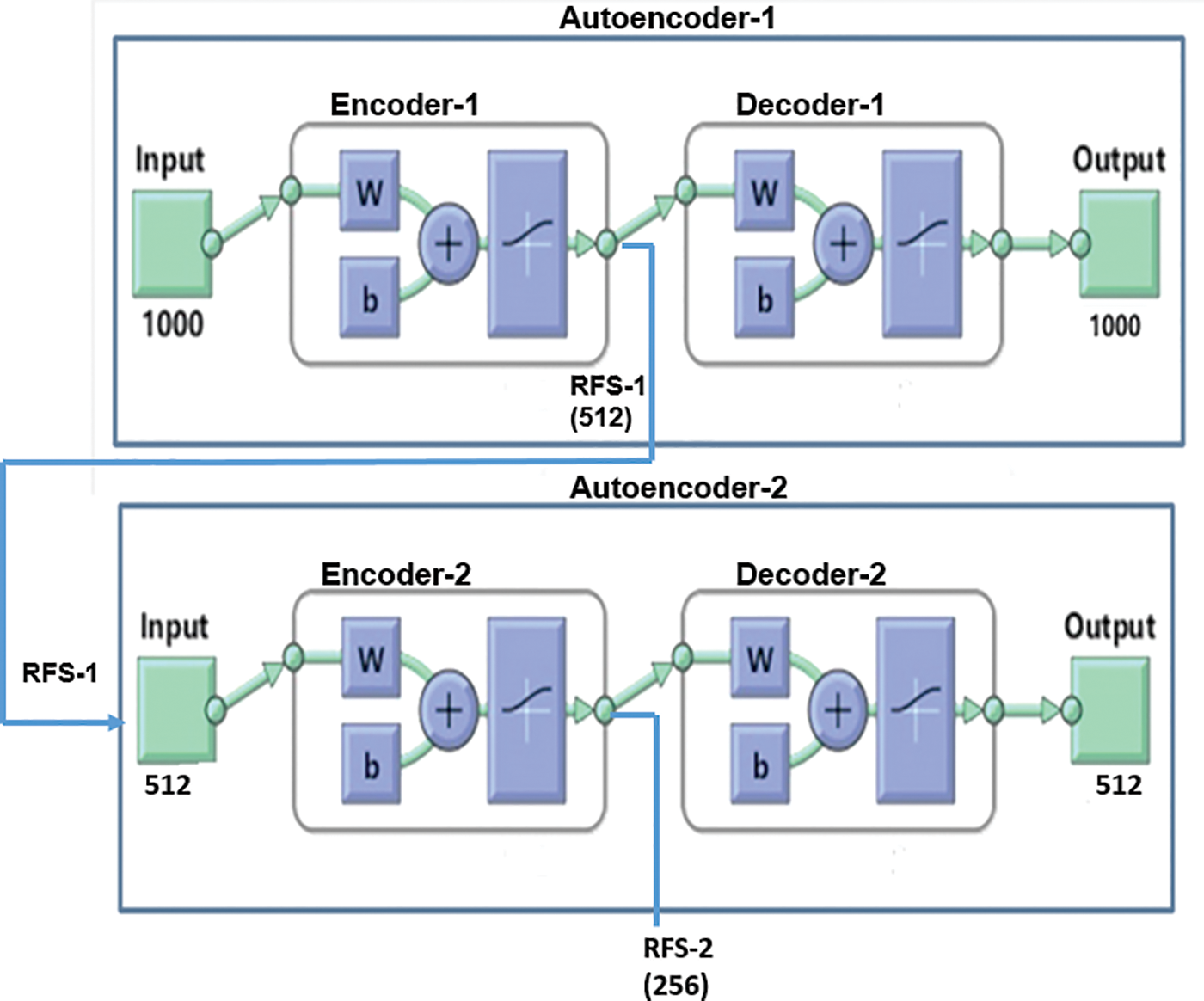
Figure 4: Sparse autoencoder for dimensionality reduction

The sparse autoencoder used in this work gets trained with multiple iterations as a part of the compression procedure. The autoencoder (Autoencoder-1) is trained with training inputs received from the pre-trained models and is achieved by the Scaled Conjugate Gradient algorithm. The autoencoder determines the activation of neurons in the hidden layer based on its sparsity value. It can accomplish by applying sparse regularization to the cost function, which enables the neuron to produce an average output value. The cost function E of the autoencoder is explained as follows:

E=1M1N∑m=1M∑n=1N(xmn−xˇmn)2+λ× 'Ωweights+β× 'Ωsparsity(3)

where M is the total observations, and N is no of images in the training data, the set of training examples and its estimate is expressed as x and xˇ, sparsity and weight regularization as 'Ωweights, 'Ωsparsity, λ and β is the coefficient for weight and sparsity regularization. After training the autoencoder-1, Reduced Feature Set-1 (RFS-1) is extracted from the encoder-1 and discards the decoder-1. The second autoencoder (Autoencoder-2) is also trained in the same way, using RFS-1 as its input to get the second feature set called Reduced Feature Set-2 (RFS-2). In the current work, the sparsity and weight regularization proportions are set as λ=0.004, β = 4. Numerous experiments were conducted and recorded to establish the aforementioned values for each parameter. The one which achieves the best is utilized in work. The flow of feature extraction and reduction is shown in Fig. 5.

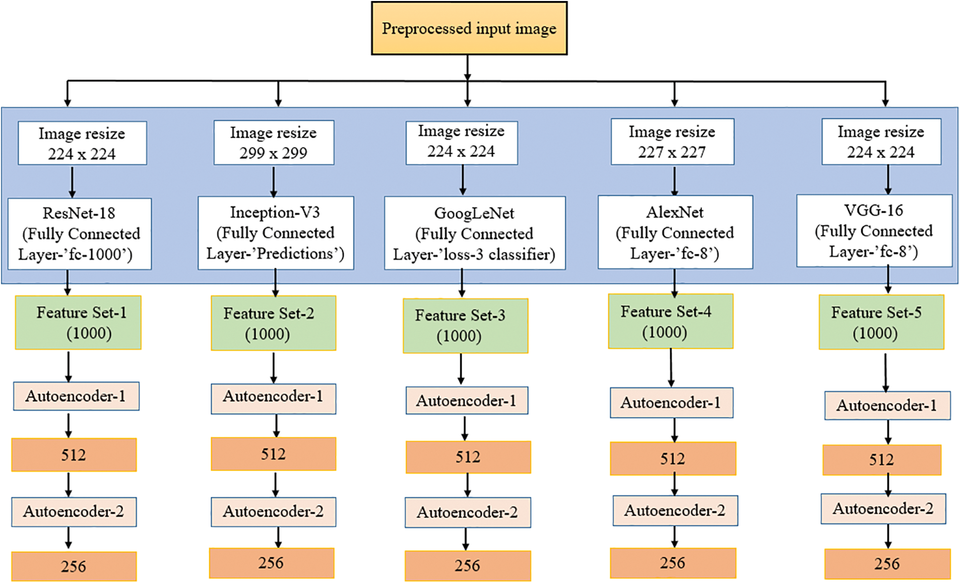
Figure 5: Feature extraction and reduction

4.3 Deep Neural Network Classification

Deep neural networks evolved from a multilayer variation of the artificial neural network. Recently, deep neural networks have become the go-to method for resolving numerous computer vision issues. Deep neural networks (DNNs) involve arranging layers of neural networks along the depth and width of smaller structures. DNNs are a potent class of machine learning techniques. Due to their remarkable ability to learn both the internal mechanisms of the input data vectors and the nonlinear input-output mapping, the DNN models have recently gained immense popularity. As the network goes deeper, the larger the number of layers to be analyzed to obtain an optimized output. The number of hidden layers in DNN makes the framework learn more high-level, abstract input representations. The current work utilizes the DNN framework for classifying the severity stages of AD from MCI. To employ DNN for the multi-class classification, the output (RFS-2) obtained from the cascaded auto-encoder is fed into the DNN for the classification. One of the most challenging aspects of creating deep neural network models is selecting the optimum hyper-parameter while adhering to a consistent approach to increase the model's dependability and effectiveness. The DNN framework is tuned and trained with multiple iterations and hyperparameters to achieve supreme performance. Table 3 displays a view of the model’s experiment with various hyper-parameters.

5  Performance Evaluation Metrics

The model’s performance in classification can assess using the performance metric. As a medical application, the classifier must be able to identify the presence or absence of the disease correctly. Therefore, the performance indicators considered for the current work, such as accuracy, precision, recall, and F1 score, are crucial. Accuracy (Ac) describes the accurate classification of images and the model’s performance. Precision (P) measures how well a classifier predicts the disease, while sensitivity or recall (R) focuses on the classifier’s ability to correctly identify the images without ailment. The F1 score is the harmonic mean of recall and precision. TN, TP, FP, and FN represent the number of true negatives, true positives, false positives and false negatives, respectively.

Accuracy (AC)=TP+TNTP+TN+FP+FN(4)

Precision (P)=TP(FP+TP)(5)

Recall (R)TP(FN+TP)(6)

F1-Score(F)=2×(P×R)/(P+R)(7)

6  Result and Discussion

Research has been carried out for the automatic classification of stages of AD from its very initial phase, called MCI. The collected MRI has undergone preprocessing with the Weiner filter and CLAHE for noise removal and image smoothing. The CLAHE was executed systematically so that it retrains the contrast level while enhancing the image without withdrawing any vital information from the image. The following algorithm explains a systematic method of providing the clip limit and contrast level to enhance the image. Grid the input image of the work, each grid tile has the same number of pixels and size and will not overlap.

•   For each tile, Calculate the histogram h(x), where x is the grey level ranging from 0 to L and the maximum value for L in each tile is 255.

•   Create a value to increment image contrast as ‘I’. The value of ‘I’ is directly proportional to the image enhancement. When ‘I’ increments, the higher image contrast enhancement.

•   Calculate the clip limit as cl

cl=NL+(N−N/LI)(8)

•   In each tile, the value of h(x) is calculated based on the value of cl. The cut-out pixel points are evenly allocated to the histogram of each tile. Once the pixel points are distributed. The new histogram function is represented as g(x). The following are the supporting formula for the same.

eN=∑xL(max(h(x)−cl),0)(9)

aN=eN/L(10)

where eN is the total no of pixel values exceeded the Clip Limit ‘cl′ and aN represents the increment in pixels for each grey level in the histogram.

•   The above distribution and allocation procedure will carry out until all the pixels have been cut out and allocated systematically. The following formula represents the process.

If(h(x)>uN)(11)

h(x)=c1

Else

h(x)=UN

where uN = cl – aN

•   Perform the HE on g(x) of each tile and calculate the grey level of each pixel.

The parameters of CLAHE set the clip limit of .005 and the number of tiles for the images at 64. The original and preprocessed MRI images and those with wrong values that occurred while experimenting with the procedure are shown in Fig. 6.

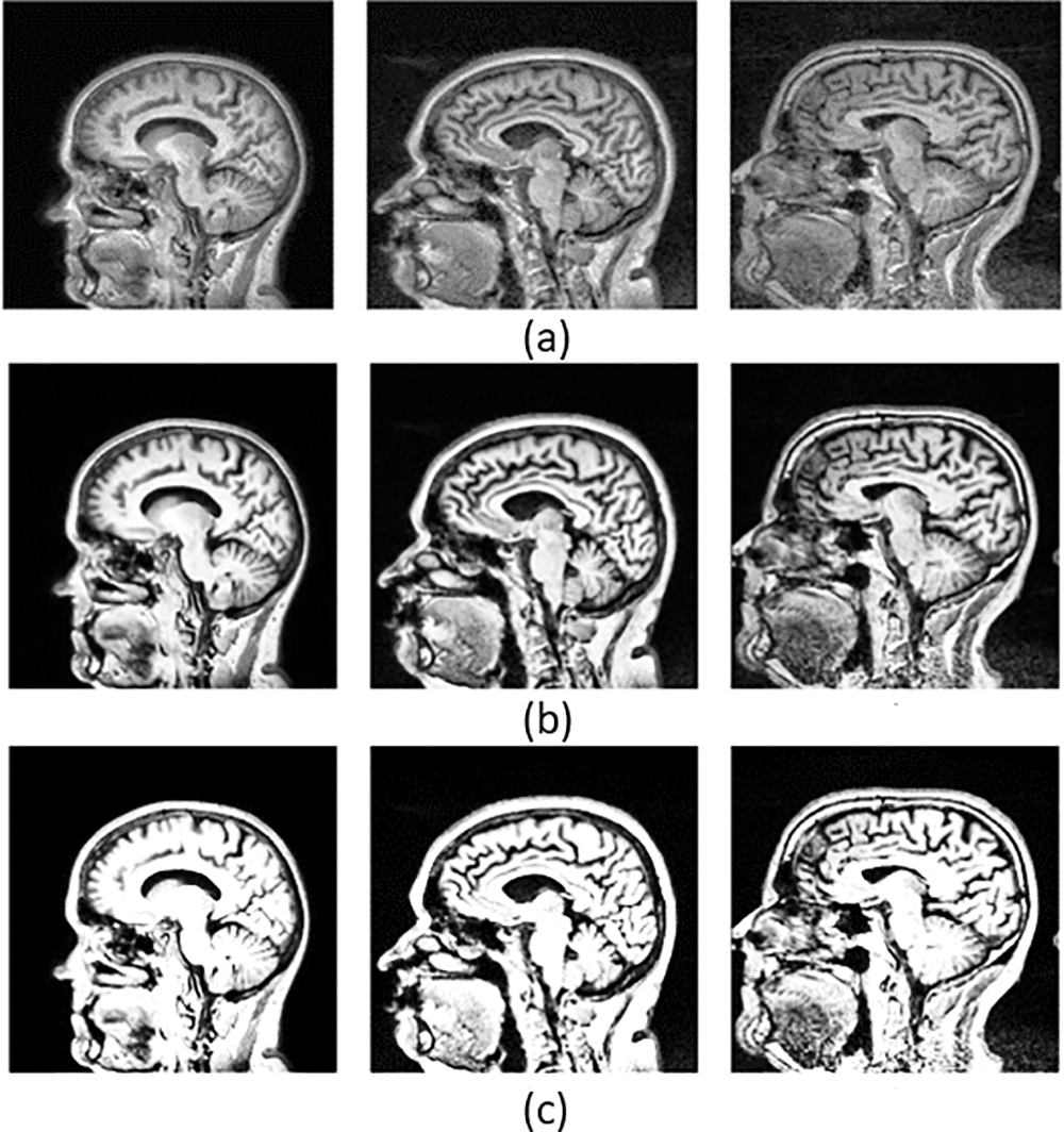
Figure 6: Represents the original images and preprocessed images with optimal and non-optimal values. Where (a) is a set of original images, (b) a preprocessed image with an optimal clip limit and retraining the contrast of the image while enhancing and also pointing out the hidden details, and (c) the set of preprocessed images with a non-optimal clip limit and which couldn’t retrain the contrast while enhancing the image

The transfer learning models utilized in the model were selected through the empirical literature review. The five models of current work are meant to extract deep features of the brain MRI. The AlexNet model used in the work encompassed eight hidden layers. Five are combined convolutional layers with the max-pooling layers, and the last three are fully connected. The current work utilizes this model by extracting the features from its third fully connected layer, FC-8. The GoogLeNet model consists of 22 deep layers with a combination of 3 convolutional, nine inception blocks with two deep layers each, and a fully connected layer called the loss-3 classifier. The third model is Inception V3, with 48 layers. Compared with v1 and v2, v3 has a deeper network, which helps optimize the network. The 11 inception modules in the Inception v3 network comprise pooling layers and convolutional filters using rectified linear units as the activation function. It has three fully connected layers, and the network conducts feature extraction from the layer named “Prediction”. The fourth model is ResNet-18. It has an architecture with 72 layers, and among those, 18 are the deep layers. It utilized the fully connected layer called “fc1000” for the extraction. The final model used in feature extraction is VGG-16 with 16 deep layers, a combination of 13 convolutional and three fully connected layers. The system experimented on ‘FC-8’ to acquire the 1000-dimensional features. A 1000-dimensional feature is obtained from each of the models.

The deep feature sets are trained with the cascaded sparse autoencoders to obtain the most reduced data representation before the plunge into the classification process. The entire layered autoencoder consists of encoder-1 with RFS-1 as 512 and encoder-2 with RFS-2 as 256. The DNN classifier trains on the reduced data to produce a multiclass categorization of AD stages. The tested data and the confusion matrix were utilized to compute the classification metrics. The experiments were conducted on an Intel i7 processor with 16 GB of RAM on Windows 10 with 64-bit to evaluate and understand the effect of pre-trained models and autoencoders with a DNN classifier for accurately classifying the stages of AD. The DNN model was set up with neural network parameters, such as input and output nodes of 256 and 5, 16 hidden layers, an Adam activation function, and 5-fold cross-validation for training and testing.

The DNN classifier model hyper tuned with relu activation function, adam optimizer, and a hidden layer configuration ranging from 1–16, with a batch size of 32 and epochs of 10, was employed on the reduced feature set of selected pre-trained models + AE and obtained a maximum accuracy of 98.54% for the ResNet-18. As the number of layers increases, the accuracy of the performance of the model starts to decline, and the experimentation process and its results state that the model performed invariantly well with the configuration of 12 hidden layers. Table 4 shows the range of accuracies obtained for all five pre-trained models with autoencoders.

The performance metrics for the Multiclass of AD stages with DNN and transfer learning model are depicted in Table 5. The study indicates that ResNet-18 + AE with DNN stands out by achieving optimum results in the classification when compared to other models. It could obtain an average performance of 98.98% in precision, 98.90% in the recall, and 98.82% with an F1 score. ResNet’s + AEs deep learning framework’s potential made it swiftly rise to prominence, as it is one of the most popular approaches to various computer vision issues due to its exceptional abilities and characteristics in feature extraction and image recognition. The model has used five-fold cross-validation with the training and testing process.

The model Fig. 7 represents the Confusion Matrix (CM) of the proposed models for predicting the true positive and true negative values for the five stages of Alzheimer’s Disease. CM depicts the tabular performance of GoogLeNet + AE, AlexNEt + AE, Inception V3 + AE, ResNet-18 + AE, and VGG-16 + AE for the multi-classification of the disease.

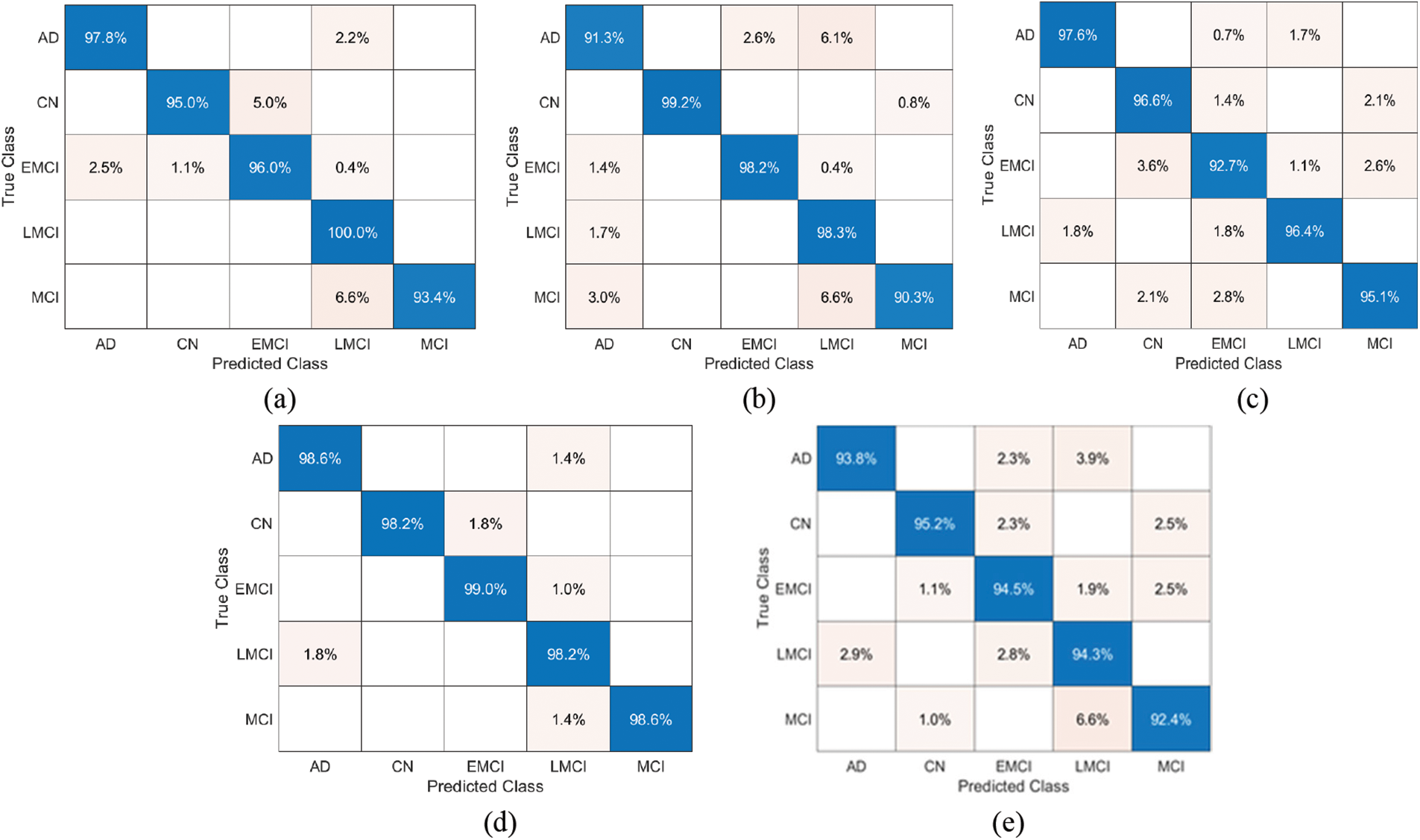
Figure 7: Confusion Matrix for the proposed classification of stages of Alzheimer’s disease: (a) AlexNet + AE+DNN, (b) GoogLeNet + AE+DNN, (c) Inception-V3 + AE+DNN, (d) ResNet-18 + AE+DNN, (e) VGG-16 + AE+DNN

The Receiver Operating Characteristic (ROC) helps visualize the classifier’s performance and summarize how well the classifier can distinguish the five classes. The following Fig. 8 shows the ROC curve obtained for ResNet with DNN.

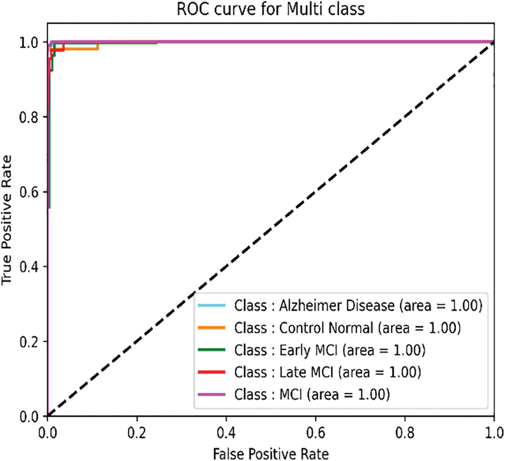
Figure 8: ROC curve of the ResNet + AE+DNN

The findings of the suggested approach’s quantitative comparison with the most cutting-edge outcomes explained in Table 6 are to gauge the effectiveness of the method. The comparison is based on the dataset, the number of classes and the accuracy of each model acquired according to its maximum level. Based on the comparison, the suggested technique performs well on the ADNI dataset. The results of the experiments confirm the accuracy and efficiency of AD Classification from its initial phase and the potential of the suggested methods. Also, the results show that the transfer learning models with AE and DNN are quite promising and convincing because they could get reliable feature information from MRI and achieve multi-class classification in stages of AD. The computational complexity of the ReseNet-18 + AE+DNN model was 11.5 sec/epochs for training and 6.4 sec/epochs for testing.

7  Conclusion

An essential component of dementia diagnosis, particularly for the aged population, is AD classification. This work proposes transfer learning models and cascaded autoencoders with DNN-based methods to apply AD Classification. The approach has an optimum classification accuracy of 98.54%, recalls of 98.90%, a precision of 98.98%, and an F1 score of 98.82%. The system achieved a 5-way classification of the disease as AD, CN, MCI, EMCI, and LMCI. The combination of 3D input image preprocessing, feature extraction and reduction, and classification with the proposed model ensure that the approach is promising to obtain supreme performance for an early onset category of the population. The results of this study demonstrate that the proposed model outperformed other classification models and are shown in the state-of-the-art table. In the future, the model can attempt to estimate the time required to convert a patient from an MCI stable stage to a protracted stage. It could aid the practitioner and the patient in ensuring that the right course of therapy is followed. Future research can work in the same area to predict the conversion of subjects from MCI to AD with promising bio-inspired algorithms such as monarch butterfly optimization (MBO), earthworm optimization algorithm (EWA), elephant herding optimization (EHO), moth search (MS) algorithm. Gene and blood protein data, MR images, and electronic health records can all be put together to predict better and classify disease stages and build complete e-health.

Funding Statement: The authors received no specific funding for this study.

Conflicts of Interest:The authors declare that they have no conflicts of interest to report regarding the present study.

References

1. A. Sanabria-Castro, I. Alvarado-Echeverría and C. Monge-Bonilla, “Molecular pathogenesis of Alzheimer’s disease: An update,” Annals of Neurosciences, vol. 24, no. 1, pp. 46–54, 2017. [Google Scholar] [PubMed]

2. S. Spasov, L. Passamonti, A. Duggento, P. Liò and N. Toschi, “A parameter-efficient deep learning approach to predict conversion from mild cognitive impairment to Alzheimer’s disease,” NeuroImage, vol. 189, pp. 276–287, 2019. [Google Scholar] [PubMed]

3. F. Gao, H. Yoon, Y. Xu, D. Goradia, J. Luo et al., “AD-NET: Age-adjust neural network for improved MCI to AD conversion prediction,” NeuroImage Clinical, vol. 27, no. 3, pp. 102290, 2020. [Google Scholar] [PubMed]

4. G. Lee, K. Nho, B. Khang, K. A. Sohn and D. Kim, “Predicting Alzheimer’s disease progression using multi-modal deep learning approach,” Scientific Reports, vol. 9, no. 1, pp. 1–12, 2019. [Google Scholar]

5. J. Venugopalan, L. Tong, H. R. Hassanzadeh and M. D. Wang, “Multimodal deep learning models for early detection of Alzheimer’s disease stage,” Scientific Reports, vol. 11, no. 1, pp. 1–13, 2021. [Google Scholar]

6. J. Islam and Y. Zhang, “A novel deep learning based multi-class classification method for Alzheimer’s disease detection using Brain MRI data,” in Int. Conf. on Brain Informatics, Padova, Italy, pp. 213–222, 2017. [Google Scholar]

7. S. Basaia, F. Agosta, L. Wagner, E. Canu, G. Magnani et al., “Automated classification of Alzheimer’s disease and mild cognitive impairment using a single MRI and deep neural networks,” NeuroImage: Clinical, vol. 21, pp. 101645, 2019. [Google Scholar] [PubMed]

8. J. Arunnehru and M. K. Geetha, “Automatic human emotion recognition in surveillance video,” Intelligent Techniques in Signal Processing for Multimedia Security, vol. 660, no. 10, pp. 321–342, 2017. [Google Scholar]

9. D. K. Oommen and J. Arunnehru, “A comprehensive study on early detection of Alzheimer disease using convolutional neural network,” in Int. Conf. on Advances in Materials, Computer and Communication Technologies, Kanyakumari, India, vol. 2385, pp. 50012, 2022. [Google Scholar]

10. N. Mahendran and V. P. M. Durairaj, “A deep learning framework with an embedded-based feature selection approach for the early detection of the Alzheimer’s disease,” Computers in Biology and Medicine, vol. 141, no. 2, pp. 105056, 2022. [Google Scholar] [PubMed]

11. Z. Qin, Z. Liu, Q. Guo and P. Zhu, “3D convolutional neural networks with hybrid attention mechanism for early diagnosis of Alzheimer’s disease,” Biomedical Signal Processing and Control, vol. 77, no. 3, pp. 103828, 2022. [Google Scholar]

12. D. Oommen and J. Arunnehru, “Early diagnosis of Alzheimer’s disease from MRI images using Scattering Wavelet Transforms (SWT),” in Int. Conf. on Soft Computing and its Engineering Applications, Gujarat,India, vol. 1572, pp. 249–263, 2022. [Google Scholar]

13. J. Arunnehru and M. K. Geetha, “Motion intensity code for action recognition in video using PCA and SVM,” in Mining Intelligence and Knowledge Exploration, Tamil Nadu, India, vol. 8284, pp. 70–81, 2013. [Google Scholar]

14. M. A. Ebrahimighahnavieh, S. Luo and R. Chiong, “Deep learning to detect Alzheimer’s disease from neuroimaging: A systematic literature review,” Computer Methods and Programs in Biomedicine, vol. 187, pp. 105242, 2020. [Google Scholar] [PubMed]

15. J. Ker, L. Wang, J. Rao and T. Lim, “Deep learning applications in medical image analysis,” IEEE Access, vol. 6, pp. 9375–9379, 2017. [Google Scholar]

16. S. Budd, E. C. Robinson and B. Kainz, “A survey on active learning and human-in-the-loop deep learning for medical image analysis,” Medical Image Analysis, vol. 71, no. 7, pp. 102062, 2021. [Google Scholar] [PubMed]

17. H. Pant, M. C. Lohani, J. Pant and P. Petshali, “GUI-based Alzheimer’s disease screening system using deep convolutional neural network,” in Computational Vision and Bio-Inspired Computing, Coimbatore, India, vol. 1318, pp. 259–272, 2021. [Google Scholar]

18. D. Ushizima, Y. Chen, D. Ovando, M. Alegro, R. Eser et al., “Deep learning for Alzheimer’s disease: Mapping large-scale histological Tau Protein for neuroimaging biomarker validation,” NeuroImage, vol. 248, no. 3, pp. 118790, 2022. [Google Scholar] [PubMed]

19. W. Li, G. G. Wang and A. H. Gandomi, “A survey of learning-based intelligent optimization algorithms,” Archives of Computational Methods in Engineering, vol. 28, pp. 3781–3799, 2021. [Google Scholar]

20. W. Li and G. G. Wang, “Elephant herding optimization using dynamic topology and biogeography-based optimization based on learning for numerical optimization,” Engineering with Computers, vol. 38, no. S2, pp. 1585–1613, 2022. [Google Scholar]

21. K. Oh, Y. C. Chung, K. W. Kim, W. S. Kim and I. S. Oh, “Classification and visualization of Alzheimer’s disease using volumetric convolutional neural network and transfer learning,” Scientific Reports, vol. 9, no. 1, pp. 1–16, 2019. [Google Scholar]

22. K. R. Kruthika and H. D. Maheshappa, “CBIR system using capsule networks and 3D CNN for Alzheimer’s disease diagnosis,” Informatics in Medicine Unlocked, vol. 14, no. 1, pp. 59–68, 2019. [Google Scholar]

23. D. Pan, A. Zeng, L. Jia, Y. Huang, T. Frizzell et al., “Early detection of Alzheimer’s disease using magnetic resonance imaging: A novel approach combining convolutional neural networks and ensemble learning,” Frontiers in Neuroscience, vol. 14, pp. 259, 2020. [Google Scholar] [PubMed]

24. Y. Gupta, R. K. Lama and G. R. Kwon, “Prediction and classification of Alzheimer’s disease based on combined features from apolipoprotein-E genotype, cerebrospinal fluid, MR and FDG-PET imaging biomarkers,” Frontiers in Computational Neuroscience, vol. 13, pp. 72, 2019. [Google Scholar] [PubMed]

25. G. G. Wang, D. Gao and W. Pedrycz, “Solving multi objective fuzzy job-shop scheduling problem by a hybrid adaptive differential evolution algorithm,” IEEE Transactions on Industrial Informatics, vol. 18, no. 12, pp. 8519–8528, 2022. [Google Scholar]

26. A. Payan and G. Montana, “Predicting Alzheimer’s disease a neuroimaging study with 3D convolutional neural networks,” in Pattern Recognition Applications and Methods Conf. Proc., Lisbon, Portugal, vol. 2, pp. 355–362, 2015. [Google Scholar]

27. S. Sarraf and G. Tofighi, “Deep learning-based pipeline to recognize Alzheimer’s disease using fMRI Data,” in Future Technologies Conf. (FTC), San Francisco, United States, IEEE, pp. 816–820, 2016. [Google Scholar]

28. P. J. S. Sohi, N. Sharma, B. Garg and K. V. Arya, “Noise density range sensitive mean-median filter for impulse noise removal,” in Innovations in Computational Intelligence and Computer Vision, Singapore, vol. 1189, pp. 150–162, 2021. [Google Scholar]

29. M. T. S. A. Shukla and P. Sharma, “High quality of gaussian and salt & pepper noise remove from MRI Image using modified median filter,” International Journal of Scientific Research & Engineering Trends, vol. 7, pp. 2395–2566, 2021. [Google Scholar]

30. T. M. S. Sazzad, K. M. T. Ahmmed, M. U. Hoque and M. Rahman, “Development of automated brain tumor identification using MRI images,” in Int. Conf. on Electrical, Computer and Communication Engineering (ECCE), Piscataway, New Jersey, pp. 1–4, 2019. [Google Scholar]

31. J. Kalyani and M. Chakraborty, “Contrast enhancement of MRI images using histogram equalization techniques,” in Int. Conf. on Computer, Electrical & Communication Engineering (ICCECE), West Bengal, India, IEEE, pp. 1–5, 2020. [Google Scholar]

32. H. Kaur and J. Rani, “MRI brain image enhancement using histogram equalization techniques,” in Int, Conf. on Wireless Communications, Signal Processing and Networking (WiSPNET), Chennai, India, IEEE, pp. 770–773, 2016. [Google Scholar]

33. H. M. Ali and M. Hanafy, “MRI medical image denoising by fundamental filters,” High-Resolution Neuroimaging-Basic Physical Principles and Clinical Applications, vol. 14, pp. 111–124, 2018. [Google Scholar]

34. Q. Meng, D. Catchpoole, D. Skillicom and P. J. Kennedy, “Relational autoencoder for feature extraction,” in Int. Joint Conf. on Neural Networks (IJCNN), Alaska, United States, IEEE, pp. 364–371, 2017. [Google Scholar]

35. J. Arunnehru, G. Chamundeeswari and S. P. Bharathi, “Human action recognition using 3D convolutional neural networks with 3D motion cuboids in surveillance videos,” Procedia Computer Science, vol. 133, no. 1, pp. 471–477, 2018. [Google Scholar]

36. R. Hedayati, M. Khedmati and M. Taghipour-Gorjikolaie, “Deep feature extraction method based on ensemble of convolutional autoencoders: Application to Alzheimer’s disease diagnosis,” Biomedical Signal Processing Control, vol. 66, no. 4, pp. 102397, 2021. [Google Scholar]

37. B. Cheng, B. Zhu and S. Pu, “Multi-auxiliary domain transfer learning for diagnosis of MCI conversion,” Neurological Sciences, vol. 43, no. 3, pp. 1721–1739, 2022. [Google Scholar] [PubMed]

38. T. Altaf, S. M. Anwar, N. Gul, M. N. Majeed and M. Majid, “Multi-class Alzheimer’s disease classification using the image and clinical features,” Biomedical Signal Processing and Control, vol. 43, no. 4, pp. 64–74, 2018. [Google Scholar]

39. A. Francis and I. A. Pandian, “Early detection of Alzheimer’s disease using ensemble of pre-trained models,” in 2021 Int. Conf. on Artificial Intelligence and Smart Systems (ICAIS), Coimbatore, India, IEEE, pp. 692–696, 2021. [Google Scholar]

40. B. Zheng, A. Gao, X. Huang, Y. Li, D. Liang et al., “A modified 3D efficientnet for the classification of Alzheimer's disease using structural magnetic resonance images,” IET Image Processing, vol. 17, no. 1, pp. 1–11, 2022. [Google Scholar]

41. K. Aderghal, K. Afdel, J. Benoispineau and G. Catheline, “Improving Alzheimer’s stage categorization with convolutional neural network using transfer learning and different magnetic resonance imaging modalities,” Heliyon, vol. 6, no. 12, pp. e05652, 2020. [Google Scholar] [PubMed]

42. H. Acharya, R. Mehta and D. K. Singh, “Alzheimer disease classification using transfer learning,” in Int. Conf. on Computing Methodologies and Communication (ICCMC), Erode, India, IEEE, pp. 1503–1508, 2021. [Google Scholar]