Performance Evaluation of Deep Dense Layer Neural Network for Diabetes Prediction

1  Introduction

Many complications in the human body, such as high blood pressure, cardiovascular diseases, renal dysfunction, visual malfunctions, eye problems, etc., can arise due to diabetes [1]. Diabetes has resulted in huge expenditures due to the increased consumption of resources for its management. Every year, diabetes results in up to five million deaths worldwide [2]. Its continuous progression and occurrence have predicted a rapid increase in cases by 2035 (International Federation, 2014) [3]. The World Health Organization (WHO) has described diabetes as a worldwide epidemic [4].

Currently, diabetes is increasing at an alarming rate and posing a significant threat to the healthy lifestyle of the human population. Higher glucose levels in the blood may cause serious diseases associated with the heart, blood vessels, nerves, kidneys, eyes, and teeth. Besides, a diabetic person is at a higher risk of developing infections [5–7]. High and better incomes in developed and developing countries are increasing sedentary lifestyles. This results in even higher diabetes risks. Maintaining better levels of blood sugar, cholesterol, and blood pressure would delay or even prevent the occurrence of diabetes. The increase in Type 1 and Type 2 diabetes globally [8] envisages the development of cost-effective methods to predict and diagnose the onset of the disease [9]. Monitoring of diabetes for its progression in terms of subsequent cardiovascular and other complications is needed. Once the diagnosis is positive, treatment goals could be set to focus on the optimum management of the disease.

Since people with a threat of diabetes require frequent observations, there is an urgent need to formulate computer models for the prognosis of the disease. Hence, this study was undertaken to predict diabetes onset using an effective combination of ML models, ensemble learning models, and the proposed DDLNN model.

The present investigation was conducted on the Diabetes dataset [10], which consists of several variables. Also, we have proposed a DDLNN with a combination of classical ML and ensemble learning algorithms for the effective prediction of diabetes disease. A comparative performance evaluation has also been performed between the proposed DDLNN, combined, and ensemble learning models to investigate which model predicts optimal results.

The significant contributions of this research work are listed below:

a.   In this study, an open diabetic dataset is used with data pre-processing techniques like standard normalization and scaling.

b.   Principal Component Analysis (PCA) has been applied to the processed dataset to reduce the number of features that are not relevant to the research.

c.   We have proposed a DDLNN model with six layers combined with classical ML models and some bagging and boosting ensemble learning.

d.   The model DDLNN used activation functions, the Rectified Unit Function (ReLU), and the Moment Estimation Optimizer (ADAM) to solve the problem of the vanishing gradient of simple CNN.

e.   Grid search K-Fold cross-validation (CV), a hyperparameter tuning model, has also been used over traditional ML models, ensemble learning models, and in the proposed DDLNN. The results before and after the hyperparameter showed a significant improvement in testing and validation accuracy.

f.   A comparative performance evaluation of the proposed DDLNN model over other learning models shows that the DDLNN has outperformed other learning models.

g.   The results of the model are also compared with the state-of-the-art models calculated on different performance metrics. The findings indicate that the model outperformed the state-of-the-art models.

While covering an introduction to diabetes disease and its types in Section 1, the remaining orchestration is followed by Section 2 for the relevant literature survey and Section 3 for the materials and methods. Section 4 describes the proposed model and the classical ML models. The detailed results and discussions are described in Section 5, and Section 6 provides the comparative analysis. Finally, we conclude the research in conjunction with the future scope in Section 7.

2  Literature Survey

Authors in [11] evaluated different ML ensembles to predict the onset of diabetes. The authors used evaluation parameters such as sensitivity, specificity, false omission rate, and Area Under the Curve (AUC) to check the effectiveness of the proposed model. They used an ensemble of two methods, adaptive boosting, and gradient boosting, for better prediction outcomes. The authors have shown the class-wise attribute distribution while demonstrating the positive and negative predictions in the dataset. However, a clear depiction of evaluation parameters and accuracy is missing.

An Artificial Neural Network model was proposed by the authors [12], prioritizing blood pressure parameters over other parameters. The model was tested with a small sample dataset. The authors gave less emphasis to the evaluation parameters when computing the best model. The procedure of distinguishing diabetic and non-diabetic patients is not explained, and a comparison with other models is required to prove the essence of the proposed model.

Authors in [13] evaluated various supervised ML algorithms on the Public Investment Management Assessment (PIMA) Indian dataset. The results were computed using the Orange Platform with Python open-source library. The authors concluded that logistic regression outperformed other ML algorithms by determining the AUC, classification accuracy, and other evaluation parameters. In this study, the best logistic regression model yielded a classification accuracy of 76.80%. However, the authors did not clearly describe the feature extraction techniques used, and the statistical techniques used failed to measure the optimal performance of the model. The performance evaluation with different parameters is also missing.

Authors in [14] conducted a systematic review in the field of diabetes research for prediction and diagnosis, complications, genetic background, and diabetes management employing ML algorithms. They suggested that SVMs are the most successful and widely used algorithms for data extraction and have proven to be necessary tools for diabetes investigation. However, the authors could have given more emphasis to the studies carried out on particular datasets. A comparative evaluation should have been done to make it easier for other researchers to reproduce the data in their studies.

The authors in [15] used random forests on the diabetes dataset for its diagnosis and showed excellent results. They proved that their results from random forest showed higher accuracy than other classification methods. However, descriptions of other machine-learning models are not provided, and they could have used more evaluation parameters to compute the best classifier. They did not apply any pre-processing technique, and a comparative evaluation of the proposed model with other models should have been done to evaluate the efficacy of the model.

Authors in [16] discussed the functioning of the KNN ML model for diabetes detection. The authors showed that the proposed algorithm provided an accuracy of 78.58% for classifying the correctness of the disease. The results were computed using the Weka tool. The authors showed an increase of 8.48% accuracy without discussing other parameters. A comparative study with other ML models is not done, which raises doubts about the proposed model’s performance. The feature selection criteria from the dataset have not been described.

In summary, a detailed study of classifiers has been performed, and the performance of the ML and ensemble learning models with various parameters has been evaluated in this research work. The research gaps found in the literature have been filled by showing a clear and concise approach to predicting the onset of diabetes. However, there are gaps in some studies, such as missing evaluation parameters, unclear feature extraction techniques, and a lack of comparative evaluations. The performance of the proposed DDLNN model is compared with other ML and ensemble learning models, but more comparative studies with other models are necessary.

3  Materials and Methods

The following section describes the materials and methodology used in this manuscript for the prediction of diabetes. This section is divided into four subsections: dataset description, proposed methodology, ML models, and evaluation parameters.

3.1 Dataset

The dataset used for predicting diabetes using various models is the PIMA Indians Diabetes Dataset [10,17]. The dataset, taken from the National Institute of Diabetes and Kidney Diseases [18], has 768 female patients over the age of 21 years.

3.2 The Proposed Methodology

The objective here is to diagnostically predict whether a patient has diabetes or not. The dataset also had certain diagnostic measures. The dataset consisted of sufficient medical diagnostic predictor variables and one target variable. The predictor variables included the patient’s number of pregnancies, body mass index (BMI), age, insulin level, etc. [19]. The foremost step is to correct the dataset, including its features, to determine the extent to which one variable is dependent on other variables. The dataset is pre-processed, and the missing entries in the dataset are filled. After applying this process, the dataset is partitioned into train-test models. The transformation strategy for the dataset was then applied. PCA was applied to find the optimal features in the dataset. In this study, 10-Fold validation was carried out on the data. Furthermore, for classification [20], various ML plus ensemble models were incorporated to evaluate the performance and effectiveness of our proposed methodology. Fig. 1 shows the framework used for diabetes prediction and classification using the various models studied in this work.

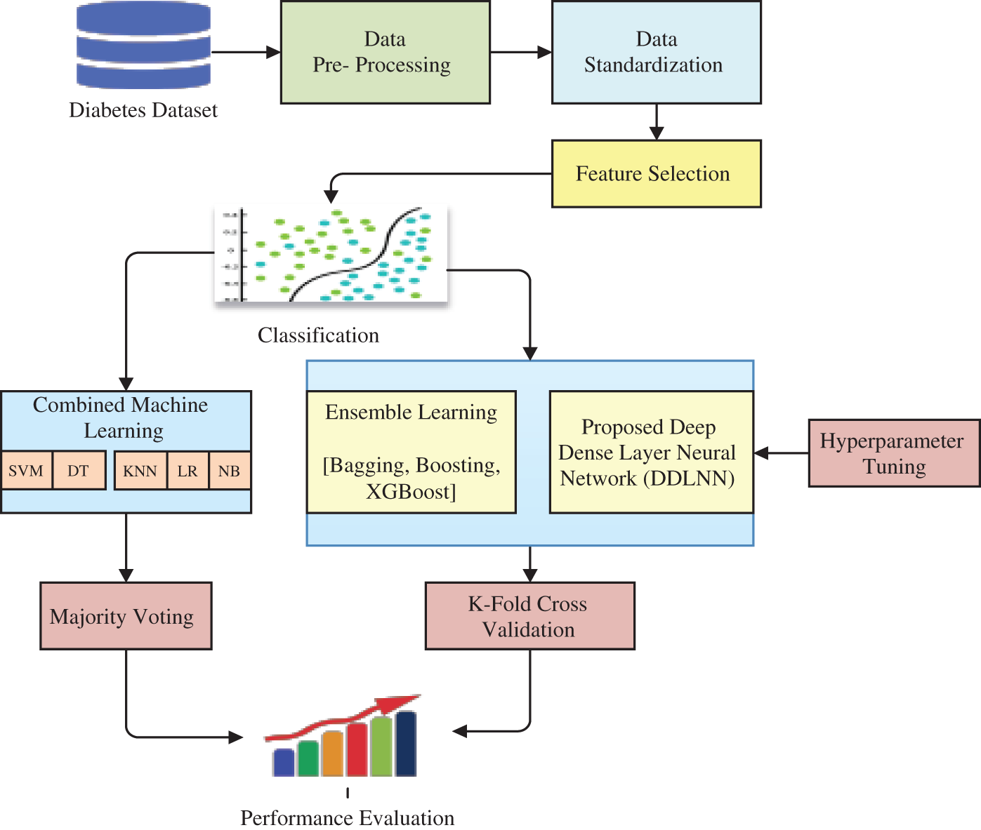
Figure 1: Framework for diabetes prediction and classification using various models

3.3 Pre-Processing

First, the dataset is pre-processed by handling missing values to forecast new data points. In the next step, standardization of the dataset to reduce computational time was performed using the standard scalar method.

Thestandardscalar,S=Value−MeanStandard Deviation(1)

The dataset had several features. Therefore, PCA, a method of dimensionality reduction [21], can be used for feature selection for representation learning and to compute the principal components of the data. PCA automatically performs the dimensionality reduction on the dataset. We can also easily plot the dataset using it.

Classification to check the accuracy of the models was carried out using various models. In addition, two ensemble methods are used, which are discussed in the next subsection.

3.4 Models Used for Deployment and Training

Ensemble methods are meta-algorithms that combine various ML methods into one predictive model. In such models, bagging is used to reduce variance and boosting to reduce bias.

3.4.1 Bagging

Bagging is a technique used in ML to strengthen weak classifiers so that they can make accurate predictions [22]. It involves using multiple weak classifiers for prediction and then combining their results through averaging or majority voting. The key objective of bagging is to ensure that the weak classifiers are independent [23] so that they predict individually and are not influenced by the predictions or errors of other classifiers.

Random Forest

The ensemble of many binary decision trees configures a Random Forest (RF) [24,25]. It was observed that to reach a terminal node, each patient had to traverse each decision tree. At the terminal node, each tree casts a vote, for example, “allergic”; the number of allergic votes out of all the votes will be the patient’s estimated allergy risk. The advantage of RF is that it is considerably less affected by noise [26,27] and helps in better generalization while reducing the variance [28].

3.4.2 Boosting

In boosting, weak classifier models work not in parallel, but sequentially. The aim is for subsequent weak classifiers to learn from the errors of the previous models [29]. The highest error appears most in the subsequent model, while a low error diminishes [30]. Decision trees, regressors, and classifiers can be considered weak classifier models [31]. However, any inappropriate selection of stopping criteria may cause overfitting.

AdaBoost

AdaBoost [31] is one of the first boosting algorithms to be adapted to explain training in ML and is suitable for converting multiple weak classifiers into a single but strong classifier [32]. It follows the sequential training principle and describes the combination of many weak learners into one prediction algorithm [33]. It can be employed to boost the performance of ML algorithms [34].

XGBoost

XGBoost [35] called extreme gradient tree boosting is an optimized distributed gradient boosting library [36], which is extremely efficient and flexible. The advantage of using the model is its lightning speed during the training and testing phases [37], as well as its capability of reducing variance [38]. Hence, it will improve the performance of the model due to the regularization parameter.

3.4.3 Combined Machine Learning Model

Combined or ensemble ML methods generally produce more accurate results than a single model. In this technique, several classical ML models, such as SVM, LR, DT, KNN, and NB classifiers, are ensembled to increase the performance of individual models by providing the best outcomes. The increased performance is obtained using the majority voting technique. Different kernels of SVM, including ‘rbf’, ‘poly’, and ‘linear’, are used. In DT, various values of the ‘max_depth’ parameter, such as 2, 3, 4, and 5, are used. In KNN, different values of the ‘n_neighbors’ parameter, such as 2, 3, and 4, are used. In LR, the ‘Penality’ parameter is set to L2, while in NB, the ‘var_smoothning’ parameter is set to ‘Le-g.’ The classifier is trained using the specified parameters, and the class is predicted using the majority vote. Fig. 2 shows the flow diagram of how different ML models are combined to predict the classification results.

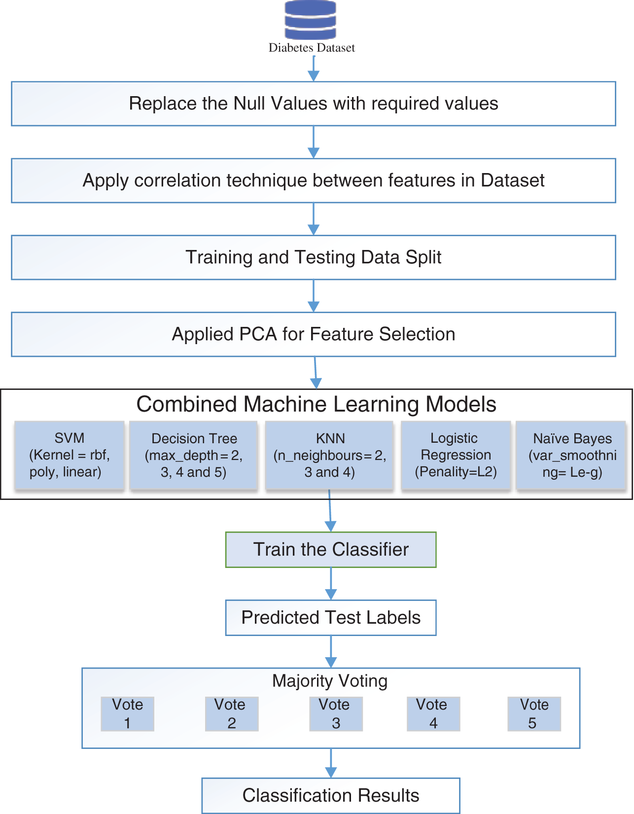
Figure 2: Illustration of combined machine learning model

4  The Proposed Model

4.1 Deep Dense Layer Neural Network

The proposed DDLNN model is inspired by the central nervous system [39] of biological neurons [40], which are used to exchange messages between the input and output [41]. The type of parameters that define DDLNN is based on:

a.   Interconnected patterns of different layers of neurons.

b.   A learning process is followed for updating the weights of the interconnections.

c.   An activation function is used for converting a neuron’s weighted input to its output activation.

Figs. 3 and 4 show the design of the model before and after hyperparameter tuning, respectively. The values computed by the model are explained in the next section.

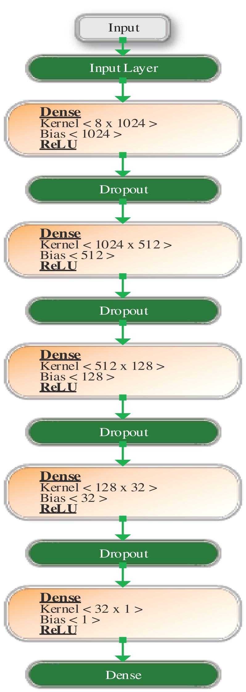
Figure 3: Architecture of DDLNN before hyperparameter tuning

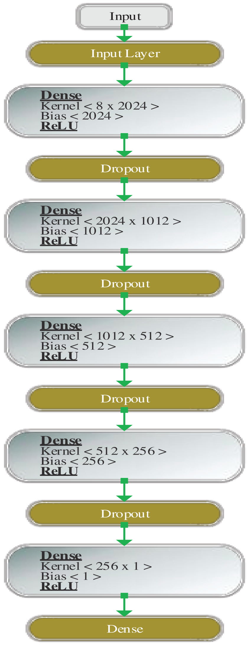
Figure 4: Architecture of DDLNN after hyperparameter tuning

Here, a sequential dense network is used because every node is connected. The proposed DDLNN has three layers: an input layer, a dense layer, and a dropout layer. The input layer receives the features of the proposed model, and ReLU is used as the activation function, which outputs 0 for a negative input and 1 for a positive input. The ADAM optimizer is used to perform optimization in the gradient descent learning rule. It takes an exponentially weighted average of gradients and solves the problem of gradient vanishing in DDLNN, and it is used because it requires less memory and is efficient.

The dense layer is a fully connected layer in which every neuron is connected to other neurons. For example, if the dense layer has a size of [8 × 1024], it means that eight dimensions are connected to 1024 nodes. The dropout layer is a layer in which a threshold limit is set, and the neurons are dropped to obtain the desired resulting output. For example, if the threshold is set to a value of 0.3, then all the nodes with greater than 0.3 values will be dropped out, and hence, the neurons will also be dropped [41].

Before hyperparameter tuning, the DDLNN model has six layers, where each layer has 8, 1024, 512, 128, 32, and 1 node, respectively. The model was trained for 50 epochs with a batch size of 20. After hyperparameter tuning, the DDLNN model has six layers, where each layer has the number of nodes as 8, 2024, 1012, 512, 256, and 1, respectively. The model was trained for 150 epochs with a batch size of 10.

4.2 Performance Evaluation Parameters

The evaluation parameters, including Matthew’s correlation coefficient (MCC) [41], are briefly described.

True positive (TP): The classifier correctly predicted a positive case, positive.

True negative (TN): The classifier correctly predicted a negative case, negative.

False positive (FP): The classifier incorrectly predicted a negative case, positive.

False negative (FN): The classifier incorrectly predicted a positive case, negative.

Accuracy: It is represented as (TP + TN)/(TP + FP + TN + FN). An accuracy of 80% means that out of 10 cases, 8 are correct and 2 are incorrect.

Precision: It is represented as TP/(TP + FP). A precision of 80% means that out of 10 allergic-labeled cases, 8 are allergic and 2 are healthy.

Recall: It is represented as TP/(TP + FN). A recall of 80% means that out of 10 allergic-labeled cases, 8 are allergic and 2 are mislabeled.

Specificity: It is represented as TN/(TN + FP). A specificity of 80% means that out of 10 healthy cases, 8 are correctly labeled as healthy and 2 are mislabelled as allergic.

MCC: It was invented by Brian Matthews in 1975, is used for model evaluation by measuring the differences between actual values and predicted values, and is represented as {(TP × TN)–(FP × FN)}/{(TP + FP) (TP + FN) (TN + FP) (TN + FN)}1/2. An MCC value of 80% means that out of 10 cases, 8 are highly correlated and 2 are not related.

4.3 Hyperparameter Tuning and Majority Voting

The validation of the proposed study is performed by comparing the testing accuracies of different ML models. Hyperparameter tuning was performed to determine the optimal parameter for each ML model. A grid search approach was applied to extract the best parameters. For example, while executing the random forest model, the parameter “n_estimators” resulted in “40” as its best parameter, whereas random forest provides comparatively better results. Similarly, the best parameter for other ML models was determined. Voting is an ensemble ML method as well. The voting ensemble in the classification problem entails aggregating the votes for crisp class labels [42] from different models and predicting the class with the largest number of votes. The research work combined SVM, LR, DT, KNN, and NB classifiers to improve the model performance. Table 1 shows different models with all parameters and their corresponding optimal parameters that have been computed using hyperparameter tuning and majority voting.

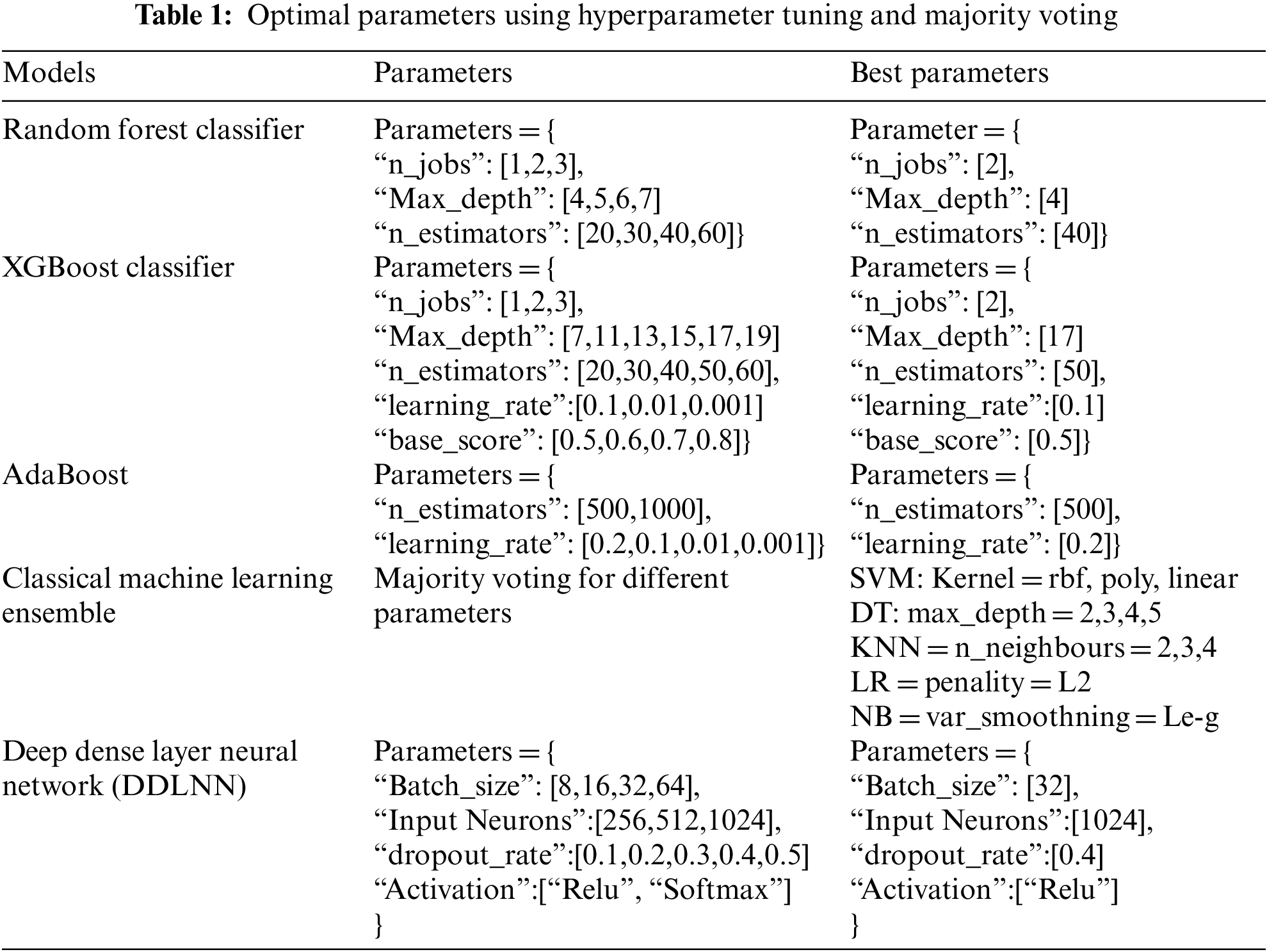
While creating a better ML model, it may not be possible to recognize the optimal parameters for the model. Hyperparameter tuning [43–46] is useful in such cases. The parameters that define the model architecture are referred to as hyperparameters. Thus, determining the ideal model architecture with optimal parameters is termed hyperparameter tuning. Among the two hyperparameter tuning methods, random search and grid search [47], grid search is a basic one [48] that is used in this paper; for random search [49], a discrete set of parameter values is provided to explore for each hyperparameter. The required number of iterations can be defined to determine the optimal parameter.

5  Results and Discussion

The models used in the research were implemented in Python using Jupyter Notebook on a 64-bit OS with an x64 CPU. The diabetes database used in the research contains 768 instances with nine variables, including pregnancies, glucose, blood pressure, skin thickness, insulin, BMI, diabetes pedigree function, age, and outcome, without any missing values. In this section, the models’ performances are evaluated through hyperparameter tuning, majority voting, and K-Fold cross-validation, followed by the results of the combined classical ML model, ensemble models, and the proposed DDLNN model. We compare the performance evaluation of various models based on different evaluation parameters [50–55].

5.1 K-Fold Validation

During the training phase, the actual model performance cannot be assessed correctly whether it has obtained the desired level of accuracy or not. So, a model validation technique is used to validate the accuracy of the training model with the test data [56]. To evaluate the actual performance of models, they are tested on an unseen dataset. Therefore, cross-validation was used to test the effectiveness of any model [57,58]. The K-Fold method uses easily understandable procedures [59] and, in general, results in a model that has a lower bias than other methods [60,61]. It guarantees that all the study of the data from the original dataset is an opportunity to emerge in the testing and training set of the dataset. This approach performs well if the input data size is small. The method uses the steps described below:

a.   The entire dataset is split into K-Folds, where the value of K should not be too small or too high. In general, 5 to 10 folds of the dataset are chosen depending on the size of the data. If a high value of k is selected, it leads to a less biased model, but a large variance can be a reason for overfitting. On the contrary, the smaller value of K is similar to the training and testing split approach previously considered.

b.   In the second step, the model was fitted by the K-1 fold, and the model was validated using the remaining Kth fold.

c.   This process was performed until every K-Fold was provided with the test set of the dataset.

d.   After this process, the average of the recorded scores was calculated. This score is the performance metric of the model.

Cross-validation was performed to achieve higher testing accuracies. In addition, to certify bias and variance, where bias is low but the variance is high, cross-validation is used. Table 2 shows the validation accuracies for K values ranging from 1 to 10 for different ML models before hyperparameter tuning.

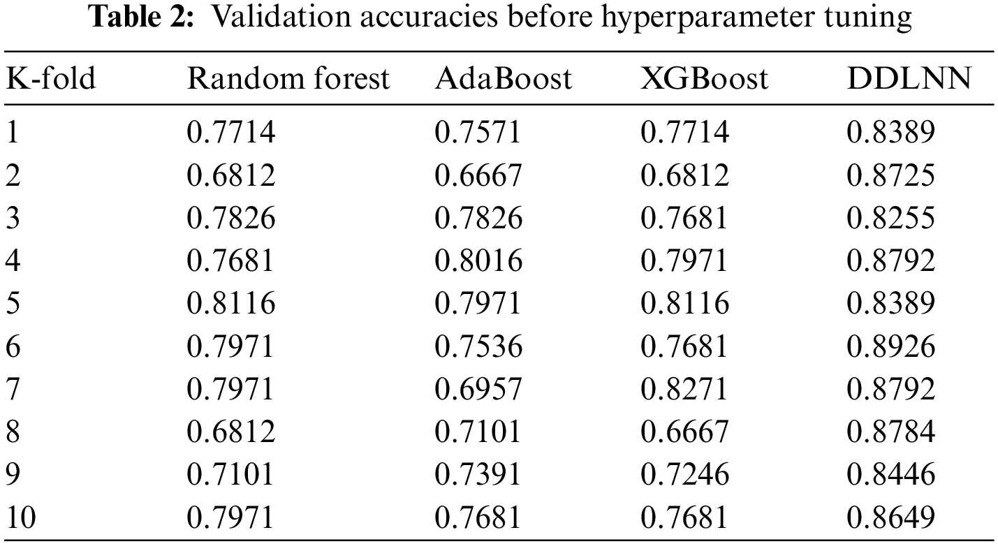
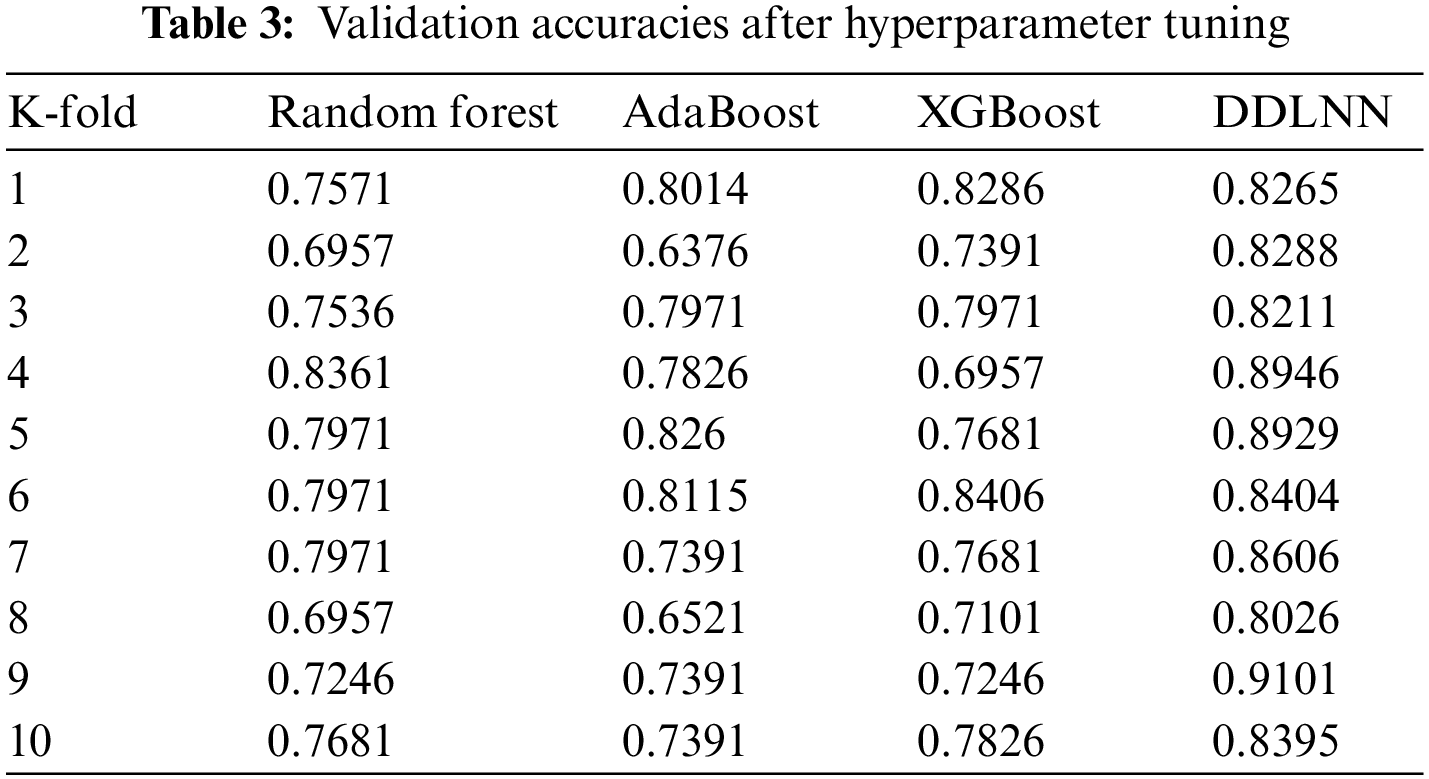
Table 3 shows the validation accuracies for K values ranging from 1 to 10 for different ML models after hyperparameter tuning.

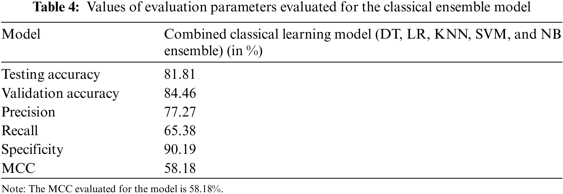
5.2 Results of the Combined Machine Learning Model

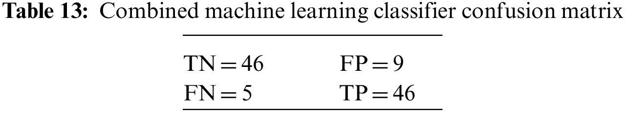
The classical ML ensemble model, after majority voting, shows an accuracy of 81.81% and a precision of 77.27%. These results, along with the values of other evaluation parameters, are shown in Table 4.

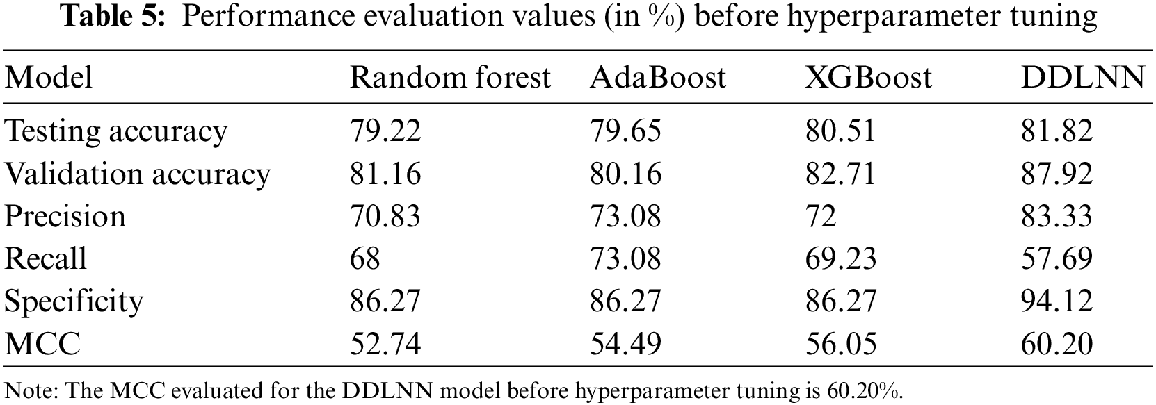
5.3 Results of Ensemble and Proposed DDLNN Before Hyperparameter Tuning and Cross-Validation

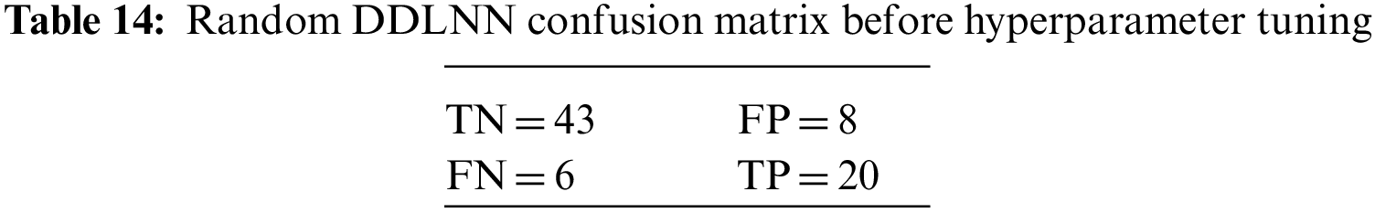
The DDLNN model used six layers, with each subsequent layer having 8, 1024, 512, 128, 32, and 1 node(s), respectively. The model was trained for 50 epochs with a batch size of 20, resulting in an accuracy of 81.82%. In the RF bagging classifier, the test train is set to 90:10. Table 5 shows the evaluation parameters obtained before hyperparameter tuning for the proposed model and the classifiers RF, AdaBoost, and XGBoost.

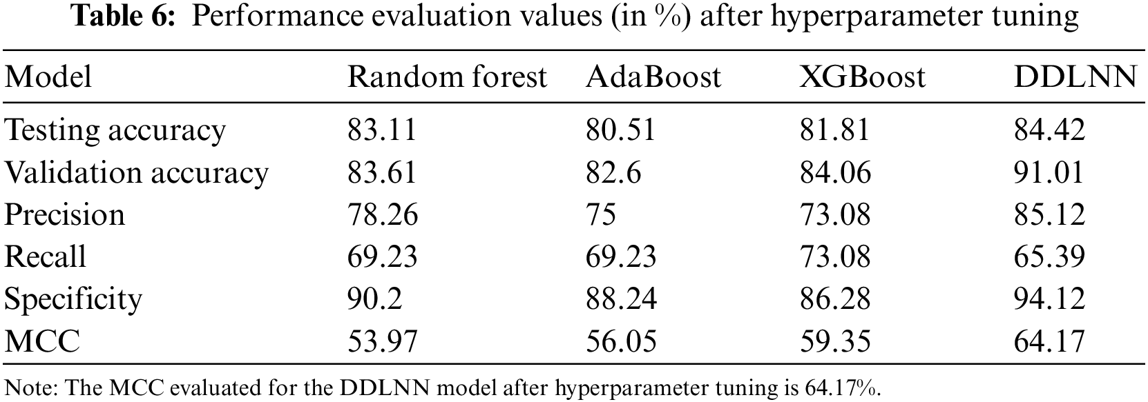
5.4 Results of Ensemble and Proposed DDLNN After Hyperparameter Tuning and Cross-Validation

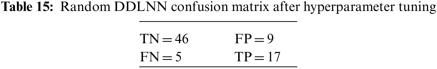
The DDLNN model used six layers, with each subsequent layer having 8, 2024, 1012, 512, 256, and 1 node(s), respectively. The model was trained for 150 epochs with a batch size of 10. The resulting accuracy is 84.42%, which achieved optimal outcomes. Table 6 shows the evaluation parameters obtained after hyperparameter tuning for the proposed DDLNN model and the classifiers RF, AdaBoost, and XGBoost.

6  Comparative Analysis

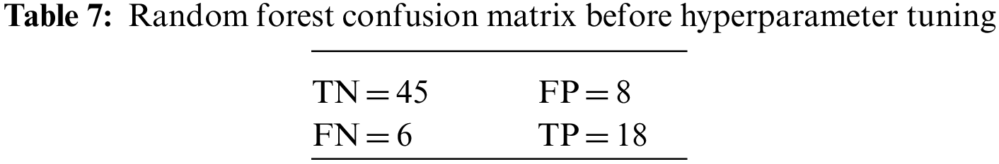
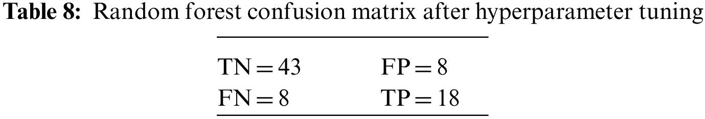
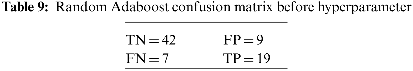
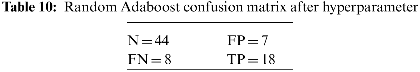
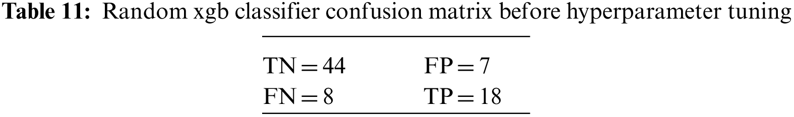
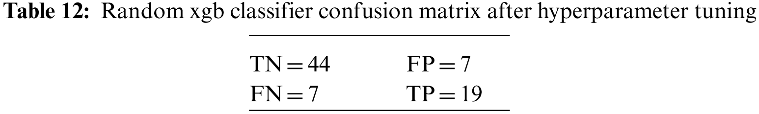
An N × N matrix called a confusion matrix is used to evaluate the performance of classification algorithms. The matrix can be used to calculate global estimations such as accuracy, precision, recall, specificity, and MCC. The 2 × 2 confusion matrices before and after hyperparameter tuning for the various classification models are presented in Tables 7 to 15.

6.1 Comparative Performance of DDLNN with Other Learning Models

A comparative performance analysis of the proposed DDLNN model with other learning models based on accuracy has been performed and shown in Table 16.

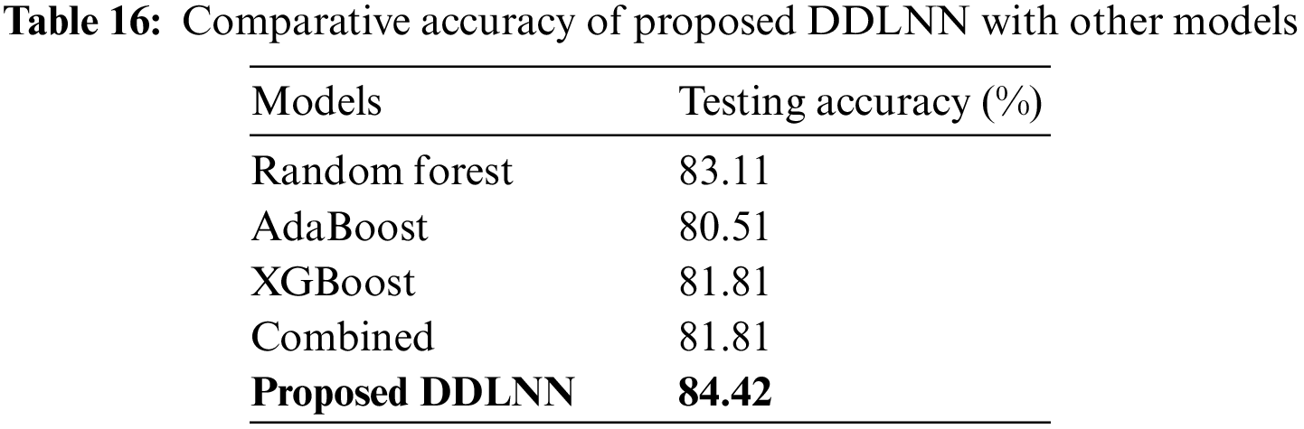
So, it is evident that DDLNN outperforms other models.

6.2 Comparison of Proposed DDLNN with State-of-the-Art Works

A comparative performance analysis of the proposed DDLNN model with recently published work based on the accuracy of models has been performed and is shown in Table 17.

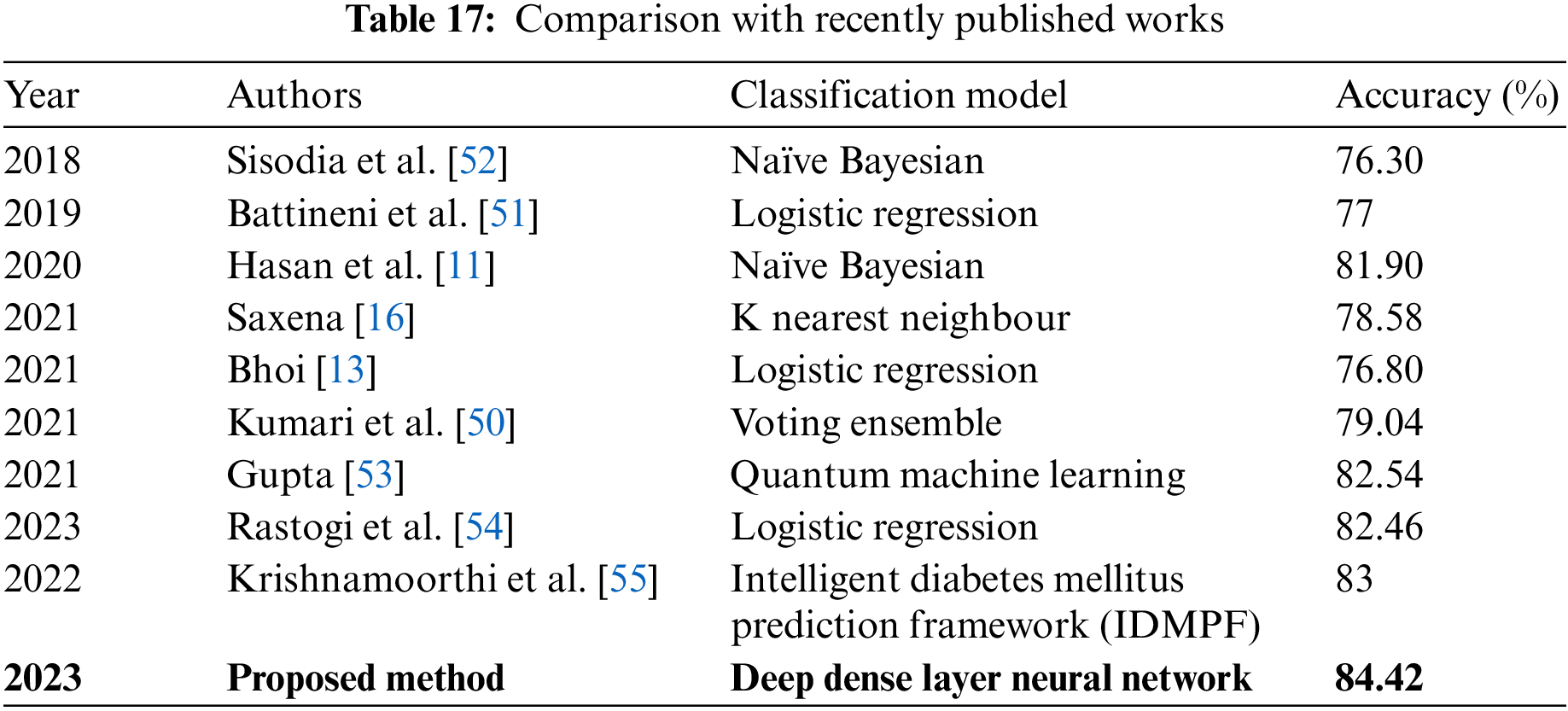
The outcomes demonstrate that the proposed model outperforms other recently published models. We also compared the results of our proposed model with those of existing ML algorithms, as shown in Table 16, which demonstrates the overall higher accuracy of our proposed model. The main reason for our proposed model outperforming the state-of-the-art is that we used a deep, dense, layered network in which each neuron is connected to other neurons. The model updates the weights of the interconnections and avoids the problem of vanishing gradient.

7  Conclusion and Future Work

The proposed DDLNN model uses six layers, where each subsequent layer has eight, 2024, 1012, 512, 256, and 1 node(s) respectively. The model was trained for 150 epochs with a batch size of 10. After hyperparameter tuning, the model yielded the highest accuracy of 84.42%, outperforming other models and the recently published state-of-the-art. The authors conclude that ML models perform better after hyperparameter tuning or the grid search approach. Therefore, incorporating hyperparameter tuning to determine the optimal parameters for the corresponding models is useful. Moreover, these techniques can be used in commercial disease detection systems to diagnose diseases and distinguish the semantic relationships between them, leading to better prescriptions.

Models for disease prediction are expected to have a few false positives for maximizing recall. Resampling and data augmentation will be used to enhance the recall rate of the DDLNN model in the future. The model can also be trained and tested for other disease predictions. Early prediction of chest and heart diseases can be implemented in our ongoing research. Multi-class classification can also be used in future illness prediction models by selecting features from many datasets. To further enhance the prediction performance of models, more efficient classification techniques can be explored, including developing and enhancing a model classification for a categorical dataset. Deep learning techniques such as CNN and Generative Adversarial Networks can be used to forecast additional diseases using more features.

Funding Statement: The authors received no specific funding for this study.

Availability of Data and Materials: The PIMA Indian diabetes dataset is available in the public domain. The python code for the prediction of diabetes using described models is uploaded on: https://github.com/niha2211/Diabetes_Prediction_hyperparameter_tuning.git to enhance the usability of the proposed technique. Access can be provided to the readers upon requesting the authors.

Conflicts of Interest: The authors declare that they have no conflicts of interest to report regarding the present study.

References

1. E. Lieth, T. W. Gardner, A. J. Barber and D. A. Antonetti, “Retinal neurodegeneration: Early pathology in diabetes,” Clinical & Experimental Ophthalmology: Viewpoint, vol. 28, no. 1, pp. 3–8, 2000. [Google Scholar]

2. B. Jonsson, “The economic impact of diabetes,” Diabetes Care, vol. 2, no. Supplement 3, pp. 7–10, 1998. [Google Scholar]

3. F. Lecky, J. Benger, S. Mason, P. Cameron and C. Walsh, “The international federation for emergency medicine framework for quality and safety in the emergency department,” Emergency Medicine Journal, vol. 31, no. 11, pp. 926–929, 2014. [Google Scholar] [PubMed]

4. W. H. Organization, “Diabetes action now: An initiative of the World Health Organization and the international diabetes federation,” World Health Organization, 2004. https://apps.who.int/iris/handle/10665/42934 [Google Scholar]

5. S. Wang, P. Ma, S. Zhang, S. Song and Z. Wang, “Fasting blood glucose at admission is an independent predictor for 28-day mortality in patients with COVID-19 without previous diagnosis of diabetes: A multi-centre retrospective study,” Diabetologia, vol. 63, no. 10, pp. 2102–2111, 2020. [Google Scholar] [PubMed]

6. Y. Chen, D. Yang, B. Cheng, J. Chen and A. Peng, “Clinical characteristics and outcomes of patients with diabetes and COVID-19 in association with glucose-lowering medication,” Diabetes Care, vol. 43, no. 7, pp. 1399–1407, 2020. [Google Scholar] [PubMed]

7. W. Sami, T. Ansari, N. S. Butt and M. R. A. Hamid, “Effect of diet on type 2 diabetes mellitus: A review,” International Journal of Health Sciences, vol. 11, no. 2, pp. 65, 2017. [Google Scholar] [PubMed]

8. A. Moţăţăianu, S. Maier, Z. Bajko and R. B. S. Voidazan, “Cardiac autonomic neuropathy in type 1 and type 2 diabetes patients,” BMC Neurology, vol. 18, no. 1, pp. 1–9, 2018. [Google Scholar]

9. E. P. Thong, D. P. Ghelani, P. Manoleehakul, A. Yesmin, K. Slater et al., “Optimising cardiometabolic risk factors in pregnancy: A review of risk prediction models targeting gestational diabetes and hypertensive disorders,” Journal of Cardiovascular Development and Disease, vol. 9, no. 2, pp. 55. 2022. [Google Scholar] [PubMed]

10. E. Ravussin, M. E. Valencia, J. Esparza, P. H. Bennett and L. O. Schulz, “Effects of a traditional lifestyle on obesity in pimaindians,” Diabetes Care, vol. 17, no. 9, pp. 1067–1074, 1994. [Google Scholar] [PubMed]

11. M. K. Hasan, M. A. Alam, D. Das, E. Hossain and M. Hasan, “Diabetes prediction using ensembling of different machine learning classifiers,” IEEE Access, vol. 8, pp. 76516–76531, 2020. [Google Scholar]

12. S. Srivastava, L. Sharma, V. Sharma, A. Kumar and H. Darbari, “Prediction of diabetes using artificial neural network approach,” in Engineering Vibration, Communication and Information Processing, ICoEVCI 2018, India, Singapore, Springer, pp. 679–687, 2019. [Google Scholar]

13. S. K. Bhoi, “Prediction of diabetes in females of pima Indian heritage: A complete supervised learning approach,” Turkish Journal of Computer and Mathematics Education (TURCOMAT), vol. 12, no. 10, pp. 3074–3084, 2021. [Google Scholar]

14. I. Kavakiotis, A. O. Tsave, N. Maglaveras and I. Vlahavas, “Machine learning and data mining methods in diabetes research,” Computational and Structural Biotechnology Journal, vol. 15, pp. 104–116, 2017. [Google Scholar] [PubMed]

15. S. Benbelkacem and B. Atmani, “Random forests for diabetes diagnosis,” in Int. Conf. on Computer and Information Sciences (ICCIS), Jouf University, Aljouf, Kingdom of Saudi Arabia, IEEE, pp. 1–4, 2019. [Google Scholar]

16. R. Saxena, “Role of k-nearest neighbour in detection of diabetes mellitus,” Turkish Journal of Computer and Mathematics Education (TURCOMAT), vol. 12, no. 10, pp. 373–376, 2021. [Google Scholar]

17. J. W. Smith, J. E. Everhart, W. C. Dickson, W. C. Knowler and R. S. Johannes, “Using the adap learning algorithm to forecast the onset of diabetes mellitus,” in Proc. of the Annual Symp. on Computer Application in Medical Care, Washington, DC (USAAmerican Medical Informatics Association, pp. 261–265, 1988. [Google Scholar]

18. L. R. Ashok, V. Latha and K. G. Sreeni, “Detection of macular diseases from optical coherence tomography images: Ensemble learning approach using vgg-16 and inception-v3,” in Proc. of Int. Conf. on Communication and Computational Technologies: ICCCT 2021, Jaipur, India, Springer, Singapore, pp. 101–116, 2021. [Google Scholar]

19. T. Filardi, F. Tavaglione, M. D. Stasio, V. Fazio and A. Lenzi, “Impact of risk factors for gestational diabetes (gdm) on pregnancy outcomes in women with gdm,” Journal of Endocrinological Investigation, vol. 41, no. 6, pp. 671–676, 2018. [Google Scholar] [PubMed]

20. Niharika and B. N. Kaushik, “Machine learning in biomedical mining for disease detection,” Journal of Artificial Intelligence, vol. 11, pp. 39–47, 2021. [Google Scholar]

21. L. Yijuan, I. Cohen, X. S. Zhou and Q. Tian, “Feature selection using principal feature analysis,” in Proc. of the 15th ACM Int. Conf. on Multimedia, Augsburg, Germany, pp. 301–304, 2007. [Google Scholar]

22. S. B. Kotsiantis, I. Zaharakis and P. Pintelas, “Supervised machine learning: A review of classification techniques,” Emerging Artificial Intelligence Applications in Computer Engineering, vol. 160, no. 1, pp. 3–24, 2007. [Google Scholar]

23. K. Hansson, S. Yella, M. Dougherty and H. Fleyeh, “Machine learning algorithms in heavy process manufacturing,” American Journal of Intelligent Systems, vol. 6, no. 1, pp. 1–13, 2016. [Google Scholar]

24. N. Altman and M. Krzywinski, “Ensemble methods: Bagging and random forests,” Nature Methods, vol. 14, no. 10, pp. 933–935, 2017. [Google Scholar]

25. S. M. Basha, H. Balaji, N. C. S. Iyengar and R. D. Caytiles, “A soft computing approach to provide recommendation on PIMA diabetes,” Heart, vol. 106, pp. 19–32, 2017. [Google Scholar]

26. A. L. Boulesteix, S. Janitza, J. Kruppa and I. R. König, “Overview of random forest methodology and practical guidance with emphasis on computational biology and bioinformatics,” Wiley Interdisciplinary Reviews: Data Mining and Knowledge Discovery, vol. 2, no. 6, pp. 493–507, 2012. [Google Scholar]

27. J. Ham, Y. Chen, M. M. Crawford and J. Ghosh, “Investigation of the random forest framework for classification of hyperspectral data,” IEEE Transactions on Geoscience and Remote Sensing, vol. 43, no. 3, pp. 492–501, 2005. [Google Scholar]

28. S. Wang, Y. Wang, D. Wang, Y. Yin and Y. Wang, “An improved random forest-based rule extraction method for breast cancer diagnosis,” Applied Soft Computing, vol. 86, pp. 105941, 2020. [Google Scholar]

29. B. Mahesh, “Machine learning algorithms-a review,” International Journal of Science and Research (IJSR), vol. 9, pp. 381–386, 2020. [Google Scholar]

30. A. Chadha and B. Kaushik, “A survey on prediction of suicidal ideation using machine and ensemble learning,” The Computer Journal, vol. 64, no. 11, pp. 1617–1632, 2021. [Google Scholar]

31. A. Shahraki, M. Abbasi and Ø. Haugen, “Boosting algorithms for network intrusion detection: A comparative evaluation of real adaboost, gentle adaboost and modest adaboost,” Engineering Applications of Artificial Intelligence, vol. 94, pp. 103770, 2020. [Google Scholar]

32. G. L. Y. Ritov, “Traffic flow prediction using adaboost algorithm with random forests as a weak learner,” International Journal of Electrical and Computer Engineering, vol. 2, no. 6, pp. 404–409, 2007. [Google Scholar]

33. R. E. Schapire and Y. Singer, “Improved boosting algorithms using confidence-rated predictions,” Machine Learning, vol. 37, no. 3, pp. 297–336, 1998. [Google Scholar]

34. D. C. Feng, Z. T. Liu, X. D. Wang, Y. Chen and J. Q. Chang, “Machine learning-based compressive strength prediction for concrete: An adaptive boosting approach,” Construction and Building Materials, vol. 230, pp. 117000, 2020. [Google Scholar]

35. T. Chen, T. He, M. Benesty, V. Khotilovich, Y. Tang et al., “Xgboost: Extreme gradient boosting,” R Package Version 0.4-2, vol. 1, no. 4, pp. 1–4, 2015. [Google Scholar]

36. L. Zhang and C. Zhan, “Machine learning in rock facies classification: An application of XGBoost,” in Int. Geophysical Conf., Qingdao, China, pp. 1371–1374, 2017. [Google Scholar]

37. R. K. Agrawal, F. Muchahary and M. M. Tripathi, “Ensemble of relevance vector machines and boosted trees for electricity price forecasting,” Applied Energy, vol. 250, pp. 540–548, 2019. [Google Scholar]

38. Y. Dong, M. Hintermüller and M. M. Rincon-Camacho, “Automated regularization parameter selection in multi-scale total variation models for image restoration,” Journal of Mathematical Imaging and Vision, vol. 40, no. 1, pp. 82–104, 2011. [Google Scholar]

39. O. S. Eluyode and D. T. Akomolafe, “Comparative study of biological and artificial neural networks,” European Journal of Applied Engineering and Scientific Research, vol. 2, no. 1, pp. 36–46, 2013. [Google Scholar]

40. Y. F. Khan, B. Kaushik, M. K. I. Rahmani and M. E. Ahmed, “Stacked deep dense neural network model to predict Alzheimer’s dementia using audio transcript data,” IEEE Access, vol. 10, pp. 32750–32765, 2022. [Google Scholar]

41. N. Srivastava, G. Hinton, A. Krizhevsky and I. Sutskever, “Dropout: A simple way to prevent neural networks from overfitting,” The Journal of Machine Learning Research, vol. 15, no. 1, pp. 1929–1958, 2014. [Google Scholar]

42. N. Gupta and B. N. Kaushik, “Prognosis and prediction of breast cancer using machine learning and ensemble-based training model,” The Computer Journal, vol. 66, no. 1, pp. 70–85, 2023. https://doi.org/10.1093/comjnl/bxab145 [Google Scholar] [CrossRef]

43. R. Bardenet, M. Brendel and B. K. M. Sebag, “Collaborative hyperparameter tuning,” in Int. Conf. on Machine Learning, PMLR, Georgia, USA, pp. 199–207, 2013. [Google Scholar]

44. S. Kaur, H. Aggarwal and R. Rani, “Hyper-parameter optimization of deep learning model for prediction of Parkinson’s disease,” Machine Vision and Applications, vol. 31, no. 5, pp. 1–15, 2020. [Google Scholar]

45. H. N. Ahuja, “Deep learning approach for diabetes prediction using PIMA Indian dataset,” Journal of Diabetes & Metabolic Disorders, vol. 19, no. 1, pp. 391–403, 2020. [Google Scholar]

46. G. T. Reddy, S. Bhattacharya, S. S. Ramakrishnan, C. L. Chowdhary and S. Hakak, “An ensemble based machine learning model for diabetic retinopathy classification,” in Int. Conf. on Emerging Trends in Information Technology and Engineering (IC-ETITE), VIT Vellore, India, IEEE, pp. 1–6, 2020. [Google Scholar]

47. N. M. Aszemi and P. D. D. Dominic, “Hyperparameter optimization in convolutional neural network using genetic algorithms,” International Journal of Advanced Computer Science and Applications, vol. 10, no. 6, pp. 269–278, 2019. [Google Scholar]

48. B. H. Shekar and G. Dagnew, “Grid search-based hyperparameter tuning and classification of microarray cancer data,” in Second Int. Conf. on Advanced Computational and Communication Paradigms (ICACCP), Sikkim, India, IEEE, pp. 1–8, 2019. [Google Scholar]

49. J. Bergstra, D. Yamins and D. Cox, “Making a science of model search: Hyperparameter optimization in hundreds of dimensions for vision architectures,” in Int. Conf. on Machine Learning, PMLR, Georgia, USA, pp. 115–123, 2013. [Google Scholar]

50. S. Kumari, D. Kumar and M. Mittal, “An ensemble approach for classification and prediction of diabetes mellitus using soft voting classifier,” International Journal of Cognitive Computing in Engineering, vol. 2, pp. 40–46, 2021. [Google Scholar]

51. G. Battineni, G. G. Sagaro, C. Nalini, F. Amenta and S. K. Tayebati, “Comparative machine-learning approach: A follow-up study on type 2 diabetes predictions by cross-validation methods,” Machines, vol. 7, no. 4, pp. 74, 2019. [Google Scholar]

52. D. Sisodia and D. S. Sisodia, “Prediction of diabetes using classification algorithms,” Procedia Computer Science, vol. 132, pp. 1578–1585, 2018. [Google Scholar]

53. H. Gupta, H. Varshney, Dr. T. K. Sharma and N. Pachauri, “Comparative performance analysis of quantum machine learning with deep learning for diabetes prediction,” Complex & Intelligent Systems, vol. 8, no. 4, pp. 3073–3087, 2022. [Google Scholar]

54. R. Rastogi and M. Bansal, “Diabetes prediction model using data mining techniques,” Measurement: Sensors, vol. 25, pp. 100605, 2023. https://doi.org/10.1016/j.measen.2022.100605 [Google Scholar] [CrossRef]

55. R. Krishnamoorthi, S. Joshi, H. Z. Almarzouki, P. K. Shukla, A. Rizwan et al., “A novel diabetes healthcare disease prediction framework using machine learning techniques,” Journal of Healthcare Engineering, vol. 2022, pp. 10, 2022. https://doi.org/10.1155/2022/1684017 [Google Scholar] [PubMed] [CrossRef]

56. H. Jin, S. Kim and J. Kim, “Decision factors on effective liver patient data prediction,” International Journal of Bio-Science and Bio-Technology, vol. 6, no. 4, pp. 167–178, 2014. [Google Scholar]

57. M. N. Triba, L. L. Moyec, C. G. R. Amathieu and N. Bouchemal, “Pls/OPLS models in metabolomics: The impact of permutation of dataset rows on the k-fold cross-validation quality parameters,” Molecular BioSystems, vol. 11, no. 1, pp. 13–19, 2015. [Google Scholar] [PubMed]

58. J. D. Rodriguez, A. Perez and J. A. Lozano, “Sensitivity analysis of k-fold cross validation in prediction error estimation,” IEEE Transactions on Pattern Analysis and Machine Intelligence, vol. 32, no. 3, pp. 569–575, 2009. [Google Scholar]

59. Y. Bengio and Y. Grandvalet, “No unbiased estimator of the variance of k-fold cross-validation,” Journal of Machine Learning Research, vol. 5, pp. 1089–1105, 2003. [Google Scholar]

60. D. Anguita, L. Ghelardoni, A. Ghio, L. Oneto and S. Ridella, “The ‘k’in k-fold cross validation,” in 20th European Symp. on Artificial Neural Networks, Computational Intelligence and Machine Learning (ESANN), Bruges, Belgium, pp. 441–446, 2012. [Google Scholar]

61. P. Tamilarasi and R. U. Rani, “Diagnosis of crime rate against women using k-fold cross validation through machine learning,” in Fourth Int. Conf. on Computing Methodologies and Communication (ICCMC), Erode, India, IEEE, pp. 1034–1038, 2020. [Google Scholar]